A Nodal Analysis Based Monitoring of an Electric Submersible Pump Operation in Multiphase Flow

Featured Application

This work can be applied in monitoring and predicting ESP failure when it operates in high gas well condition. It can be used to interpret the downhole ESP data such as pump intake pressure (PIP) and pump discharge pressure (Pdis) to diagnose ESP abnormalities related to the multiphase condition. It highlights the importance of using nodal analysis software (e.g., Schlumberger PIPESIM software) to evaluate the ESP operating condition before and after installation. It is strictly applied in the field where gas lock is a major source of the ESP abnormality.

Abstract

Electrical submersible pump (ESP) operation is compromised by free gas, resulting in premature pump failure and production losses in new wells. It is essential to detect the onset of abnormal operations. We develop a model that predicts abnormal ESP operation when the free gas level increases in the pump. The model compares operation parameters with the parameters of normal operating ranges; it shuts down the ESP when necessary. We used a Schlumberger PIPESIM software (version 2017.01) to perform nodal analysis technique; we tested the model using the other multiphase correlation model and field case studies (where the gas problem in ESP was reported). We employ a homogenous model to calculate the differential pump pressures at various gas volume fractions. Nodal analysis of the intake and discharge point predicted the commencement of abnormal ESP conditions and the associated parameters (critical gas fraction, minimum operating pump intake pressure, and pump discharge pressure). The model results were similar to other surging correlation models (e.g., Romero, Dunbar, Turpin, Cirilo, and Zhou models); they were also identical to field case studies. We identify three performance stability phases when an ESP is exposed to free gas. These are the normal and abnormal operating ranges, as well as the ESP shutdown condition. Modeling permits careful monitoring of ESP operations that can be compromised by free gas.

1. Introduction

Approximately 60% of global oil production is produced using the artificial lift (AL) pump technique; more than 20% of the pumps used are electric submersible pumps (ESPs) [1,2]. An ESP is an artificial lifting device that features multistage centrifugal pumps, a motor, seals, power cables, and surface controls. Their applications are found in both on- and off-shore production facilities [3]. This efficient downhole pump converts fluid kinetic energy to hydraulic pressure; the developed pressure depends on the pump stages and fluid properties [4,5]. The horizontal well has played a significant role in developing unconventional reservoirs. It increases the contact between the target reservoir and the production well, leading to increased flow rate and recoverable oil [6]. However, when they are new, most of these horizontal wells exhibit reductions in reservoir pressure that compromise oil production viability [7]. A previous study showed that the application of AL maintains the oil production before applying other expensive enhanced oil recovery techniques. It provides the required energy that reduces the bottom hole flowing pressure or increases the pressure drawdown. In principle, an ESP reduces the bottom hole flowing pressure; it also allows more efficient and consistent oil-lifting capacity at lower reservoir pressures than other artificial lifts. Since its invention, ESP has significantly optimized unconventional oil production [6,8]. A decrease in reservoir pressure triggers multiphase flow in a well when the pressure falls below the bubble point. Thus, the application of the ESP in a horizontal well remains a critical issue since the presence of the free gas impedes its boosting pressure [9].

The ESP was designed to manage incompressible fluid; its operation in multiphase flow caused performance degradation compared to incompressible fluid (e.g., water) [10,11]. Lea and Bearden [12] demonstrated four types of free gas effects on ESP performance: non-gas interference, gas lock interference, intermittent gas lock, and gas lock. During the first two events, an ESP exhibits minor fluctuations in the production rate, pump intake pressure (PIP), and pump discharge pressure (P_disch). When the multiphase condition develops into intermittent gas locking, ESP production significantly declines, the PIP increases, and the Pd decreases. At higher intake gas volume fraction (GVF), ESP encounters significant operation instability and vibration. After that, the impeller becomes entirely blocked by free gas, causing a gas lock. To understand the ESP stable operation condition (below the surging point), Turpin, Dunbar, Cirilo, Romero, Duran, Zhou and Sachdeva, Gamboa, and Zhu have developed an empirical correlation predicting ESP instability onset [11,13].

2. Multiphase Surging Empirical Model Review

As discussed in Section 1, several models were developed to understand the ESP operating behavior during the multiphase condition, such as dynamic and simplified empirical models used to simulate multiphase pumping behavior. However, those models require a complex solution of mass and momentum of the gas–liquid mixture in the entire ESP, and their applicability needs a detailed pump impeller and diffuser design data. Despite the developed models’ complexity and theoretical dominance, these models are still used in the industry [14]. This section presents only available critical models of judging stable and unstable (surging) ESP operation; their empirical formulas are summarized in

Table 1. Models of surging correlations.

Prediction Model	ESP Surging Correlation
Turpin et al. (1986) [15]	${\varnothing }_{Turpin}=\left(\frac{\mathbf{2000}}{\mathbf{3}PIP}\right)\frac{Q_g}{Q_l}$$, \mathrm{Assume} {\varnothing }_{Turpin}=\mathbf{1}$, initiation of abnormal operation $\frac{Q_g}{Q_l}=\frac{\mathbf{3}PIP}{\mathbf{2000}}$$, {\mathit{\lambda }}_c=\frac{Q_g}{Q_g+Q_l}$$=\frac{\left(\frac{\mathbf{3}PIP}{\mathbf{2000}}\right)}{\mathbf{1}+\left(\frac{\mathbf{3}PIP}{\mathbf{2000}}\right)}$ $Q_g$$, Q_l$$, \mathrm{are} \mathrm{gas} \mathrm{and} \mathrm{liquid} \mathrm{flow} \mathrm{rate} \mathrm{at} \mathrm{the} \mathrm{critical} \mathrm{gas} \mathrm{volume} \mathrm{fraction} [{\mathit{\lambda }}_c$]
Dunbar (1989)-Pessoa (2001) [16]	$PIP=\mathbf{935}{\left(\frac{Q_g}{Q_l}\right)}^{\frac{\mathbf{1}}{\mathbf{1.724}}}$$, \frac{Q_g}{Q_l}={\left(\frac{PIP}{\mathbf{935}}\right)}^{\mathbf{1.724}}$$, {\mathit{\lambda }}_c=\frac{Q_g}{Q_g+Q_l}$$=\frac{\left({\left(\frac{PIP}{\mathbf{935}}\right)}^{\mathbf{1.724}}\right)}{\mathbf{1}+\left({\left(\frac{PIP}{\mathbf{935}}\right)}^{\mathbf{1.724}}\right)}$
Cirilo (1998) [17]	${\mathit{\lambda }}_c=\mathbf{0.0187}PI{P}^{\mathbf{0.4342}}$
Romero (1999) [18]	${\mathit{\lambda }}_c=\mathbf{0.004}{\left(PIP-\mathbf{14.7}\right)}^{\mathbf{0.6801}}$
Duran (2003) [19]	$\frac{Q_g}{Q_{max}}=\left(\mathbf{5.580}\left(\frac{{\mathsf{\rho }}_g}{{\mathsf{\rho }}_l}\right)+\mathbf{0.098}\right){\left(\frac{Q_l}{Q_{max}}\right)}^{\mathbf{1.421}}$ $\frac{Q_g}{Q_{max}}$$\mathrm{and} \frac{Q_l}{Q_{max}}$$\mathrm{are} \mathrm{normalized} \mathrm{gas} \mathrm{and} \mathrm{the} \mathrm{liquid} \mathrm{rate} \mathrm{at} \mathrm{surging} \mathrm{point}, \mathrm{respectively}, \mathrm{and} Q_{max}$ is the maximum rate from the pump curve
Zhou (2010) [14]	$\frac{Q_l}{Q_{max}}=\mathbf{1.236426}{\left(PIP\right)}^{-\mathbf{0.34870}}{\left(\mathsf{\alpha }\right)}^{\mathbf{0.86709}}\left(\mathbf{1}-\mathsf{\alpha }\right)$ For mixed flow pump [K-70]
Gamboa (2011) [13]	$\frac{Q_g}{Q_{max}}=\mathbf{0.102}exp{\left(\frac{Q_l}{Q_{max}}\right)}^{\mathbf{4.4682}}{\left(\frac{{\mathsf{\rho }}_g}{{\mathsf{\rho }}_l}\right)}^{\mathbf{0.2}}{\left(\frac{\omega D^2}{v}\right)}^{\mathbf{0.4}}$ $\omega : \mathrm{pump} \mathrm{rotational} \mathrm{speed}, \mathrm{rpm}, v: \mathrm{fluid} \mathrm{kinetic} \mathrm{viscosity}, \mathrm{and} D$: impeller outlet diameter, m
Zhu (2017–2019) [11,20,21]	${\mathit{\lambda }}_c=\frac{\mathbf{2}{\left[\frac{\mathbf{0.4}\mathsf{\sigma }}{\left({\mathsf{\rho }}_l-{\mathsf{\rho }}_g\right)\mathsf{\delta }{R}_I}\right]}^{\mathbf{0.5}}}{{\left(\frac{\mathsf{\sigma }}{{\mathsf{\rho }}_l}\right)}^{\mathbf{0.6}}{\left(\frac{\mathbf{\Delta }{P}_{pump}{Q}_l}{{\mathsf{\rho }}_{l}V}\right)}^{-\mathbf{0.4}}{\left(\frac{{\mathsf{\rho }}_l}{{\mathsf{\rho }}_g}\right)}^{\mathbf{0.2}}}$  $\mathsf{\sigma }: \mathrm{surface} \mathrm{tension}, \mathrm{N}/\mathrm{m}, \mathsf{\delta }$$: \mathrm{Angular} \mathrm{speed},\mathrm{rad}/\mathrm{s}, V$$: \mathrm{impeller} \mathrm{volume}, m^{\mathbf{3}}$$, \mathrm{and} R_I$: represent rotator radius, m

.

Turpin [15] formulated the first empirical model to predict ESP performance in gas well conditions. Using Lea and Bearden’s experimental data [12], he developed a model to predict the surging (abnormal) initiation. His model uses the Turpin correlation (${\varnothing }_{\mathrm{Turpin}}$) parameter to judge the ESP operating condition, where the ${\varnothing }_{\mathrm{Turpin}}$ is a function of gas volume fraction and pump intake pressure. According to the author, the ESP surging condition can be initiated when (${\varnothing }_{\mathrm{Turpin}}$ > 1). Due to its simplicity, Turpin correlation is widely used to relate the ESP performance to the in situ gas and PIP to evaluate the limits of stable operation [5]. In 1989, Dunbar presented an empirical correlation for judging the pump performance in homogenous conditions. Dunbar agreed with Turpin that the PIP plays a significant role in determining critical GVF. In monitoring the ESP operation, the Dunbar model can examine the ESP performance in gas well conditions [11]. Using the mixture of air and water, Cirilo tested the two mixed flow pumps (GN4000 and GN7000) and one radial flow pump (GN2100). Cirilo presented the empirical model to compute the maximum GVF at ESP surging initiation point. The model evaluates the critical GVF as a function of the pump operating PIP [17]. Similar to the previous authors, this model can judge the ESP performance in gas well conditions.

Based on Cirilo’s experimental data, Romero developed the model to predict the multiphase head degradation of the mixed flow pump (GN4000). His model relates the critical GVF and the pump operating PIP. This model can be applied in the ESP performance monitoring since it includes the pump operating PIP [18]. Duran developed an empirical model for predicting pump performance in multiphase conditions. The model relates the normalized gas rate, normalized liquid rate, and the ratio of gas density to liquid density. The correlation predicts the stage pressure increment under the bubble flow regime and defines the transition patterns [19]. This correlation is more widely applied in designing pumps than monitoring; it is less attractive for judging the ESP performance in gassy well conditions. Using Sachdeva’s original model, Zhou (2010) developed the model to evaluate pump performance degradation in multiphase operation. His model correlated the normalized liquid rate and pump intake pressure [14]. This model can also be adopted to judge the ESP performance based on its operating PIP and normalized rate. Gamboa combined a wide range of GVFs, pump rotational speeds, and intake pressures. He developed the correlation for predicting the pump surging initiation as a function of fluid properties and rotational speed [13]. Zhu conducted the recent experimental study regarding the multiphase effect on ESP performance [11,20,21]. He developed a new mechanistic model to evaluate the gas-liquid flow patterns in the ESP. His model correlates the critical gas fraction with angular speed, surface tension, liquid flow rate, impeller volume, and rotor radius. This model is more oriented to the ESP design than monitoring operating conditions.

Briefly, the PIP plays a significant role in determining the threshold GVF amount entrained in the ESP without degradation [5]. The surging model proposed by Turpin, Dunbar, Cirilo, Romero, and Zhou offers practical parameters for judging the ESP performance in gas well conditions. The remaining correlation models were not adopted in this study.

3. ESP Fault Monitoring and Diagnosis Review

As discussed in the previous section, operating the ESP in the free gas environment results in an abnormal operation, and damages the ESP components. Unfortunately, it is impossible to limit free gas formation in the production well; however, there are several ways to control its liberation from the produced fluid. Takacs [5] demonstrated that increasing operating PIP reduces the free gas amount liberated from the produced fluid solution. Still, this approach impedes the oil production rate. Additional efforts have been subjected to ESP monitoring and diagnosis to overcome operation losses, proceed with the prevention measures, and promote abrupt free gas formation since removing and replacing a damaged pump is 40-fold more expensive than installing a new pump [22]. This section presents different perspectives for monitoring and diagnosing ESP abnormal conditions. Rensburg and Germany [23] demonstrated the usage of artificial intelligence (AI) technology to detect, diagnose, and monitor ESP abnormal behavior. They explained how the combination of artificial intelligence (AI) and Internet of Things (IoT) technologies provide an effective way to use data-driven analytics to detect the ESP abnormal behavior, based on the downhole data and providing decision support for managing the roots of the abnormal conditions. Using the field data of the 30 ESPs, they showed how the AI could provide a solution to the production disruptions caused by the several ESP failures. Unfortunately, their approach focused on the data analysis of the previous scenario to avoid future failure; this is hard to adopt in the green field where the previous failure data are not available. Oyewole [24] showed the application of real-time data processing and interpretation to reduce ESP failure. The author highlighted that a combination of the reservoir and production data results in the effective management of the ESP well. It also enhanced the oil well and reservoir monitoring, improving surveillance, analysis, and diagnosis of the ESP well. As a result, the ESP well operation was optimized, which reduced the failure likelihood. Through the presented case study (Brownfield of a Permian Basin), this approach optimized the ESP well production through downhole equipment failure reduction, early-warning detections, and reduced the equipment workover. Similar to the previous approach, it is hard to adopt it where the historical failure data are not present.

Moreover, Awaid et al. [25] employed pattern recognition analysis for ESP well surveillance. The authors developed an ESP abnormal troubleshooting checklist that quickly identifies and differentiates the root of ESP malfunction. This approach can be adapted to the new field by employing the developed checklist to diagnose ESP abnormal conditions. However, a checklist requires more attention because different failures might have the same signature; thus, ESP diagnosis can be compromised. Al-sadah et al. [26] reported that proactive ESP monitoring was possible via real-time monitoring and diagnosis. They showed that monitoring real-time data of downhole sensor readings and surface data provides a diagnostic tool that identifies ESP abnormality that could lead to shutdowns; thus, ESP trips can be prevented in advance. Agrawal et al. [27] used ESP data to monitor ESP performance, diagnose issues, and optimize production during polymer flooding. The authors combined a real-time ESP parameter alarm system, time-lapse analysis (production tubing pressure drop, pump head de-rating factor, pump, and VFD horsepower), deadhead, and multi choke test data to evaluate the most likely mechanisms leading to ESP abnormality. Their study provided a diagnostic approach to differentiate the polymer flooding plugging or gas-related failure. Based on their findings, the approach proposed can be applied in the new oil well to optimize and monitor ESP operating conditions. Nunez et al. [28] developed an ESP troubleshooting guide that reduced failures. Using monitoring information, tearing down evidence, setting configuration, and building a database with all the information of 450 oil well data, they developed a troubleshooting manual, which quickly identifies likely conditions that impede the production and performance of ESP systems.

In addition, Peng et al. [1] demonstrated that significant ESP failure happens when its key parameters start deviating from the normal operating range until an ESP stops working. They proposed an application of the principal component analysis (PCA) model to perform ESP fault detection to maintain ESP in the normal operational range. Castellanos et al. [29] showed the machine learning algorithm’s preference for future failure prediction based on historical ESP data. They adopted Classification and Regression Trees (CART) to detect and classify elementary faults in the ESP well system. CART’s proposed methodology monitored the system based on the pressure variation, flow rate, torque, and temperature. Liang et al. [30] proposed a new downhole monitoring tool, which uses an experimental phase to neutral communication scheme. In their design, an effective signal communication path is formed by the external impedance on the wellhead (connecting one phase) to the grounding ESP motor. The laboratory and field testing demonstrated the reliability of the method. Li et al. [31] proposed an online ESP fault diagnosis that combines the ESP electrical and production parameters. They designed the algorithms that perform feature extraction, combining the electrical and production parameters. This approach effectively monitored the nine typical operating fault conditions at reduced downhole sensor impact. Fusiek et al. [32] presented the three-phase optical voltage sensor for ESP monitoring. They applied a piezoelectric transducer that converts the voltage into strain. The strain is measured using a fiber Bragg grating sensor. The measured strain is amplified at the grating location and improves the measurement resolution. The electrical breakdown was minimized using the finite element electrostatic modeling software. This approach improved the electrical performance in the ESP well system. Bruijnen [33] employed a nodal, analytical, graphical method to monitor ESP well performance. He provided a general approach to assessing the ESP-assisted well based on the pump intake and discharge pressure deviation trends. However, these approaches afford diagnostic tools after abnormal conditions have occurred and provide only retrospective explanations of real-world failures.

It is essential to predict and prevent ESP failure associated with a drastic performance reduction and other problems. An effective early-warning system must be designed before ESP installation. We use Schlumberger PIPESIM software (version 2017.01) to predict ESP operation pre-installation. We consider the uncertainty imparted by multiphase well conditions. We monitor the PIP, Pd, and production rate; we compare these values (at all times) to normal reference values. Any difference predicts abnormal ESP operation. The work is novel in that we devise reference threshold values for several distinct phases of ESP operation. We used an oil well located in the Delaware Basin to evaluate the model. To generalize the model, we evaluated different types of wells. For example, an ESP deployed in a dead well was used to stimulate production; an ESP installed in a naturally flowing well served to increase production. We consider both single-phase and multiphase conditions inside the pump.

4. Materials and Methods

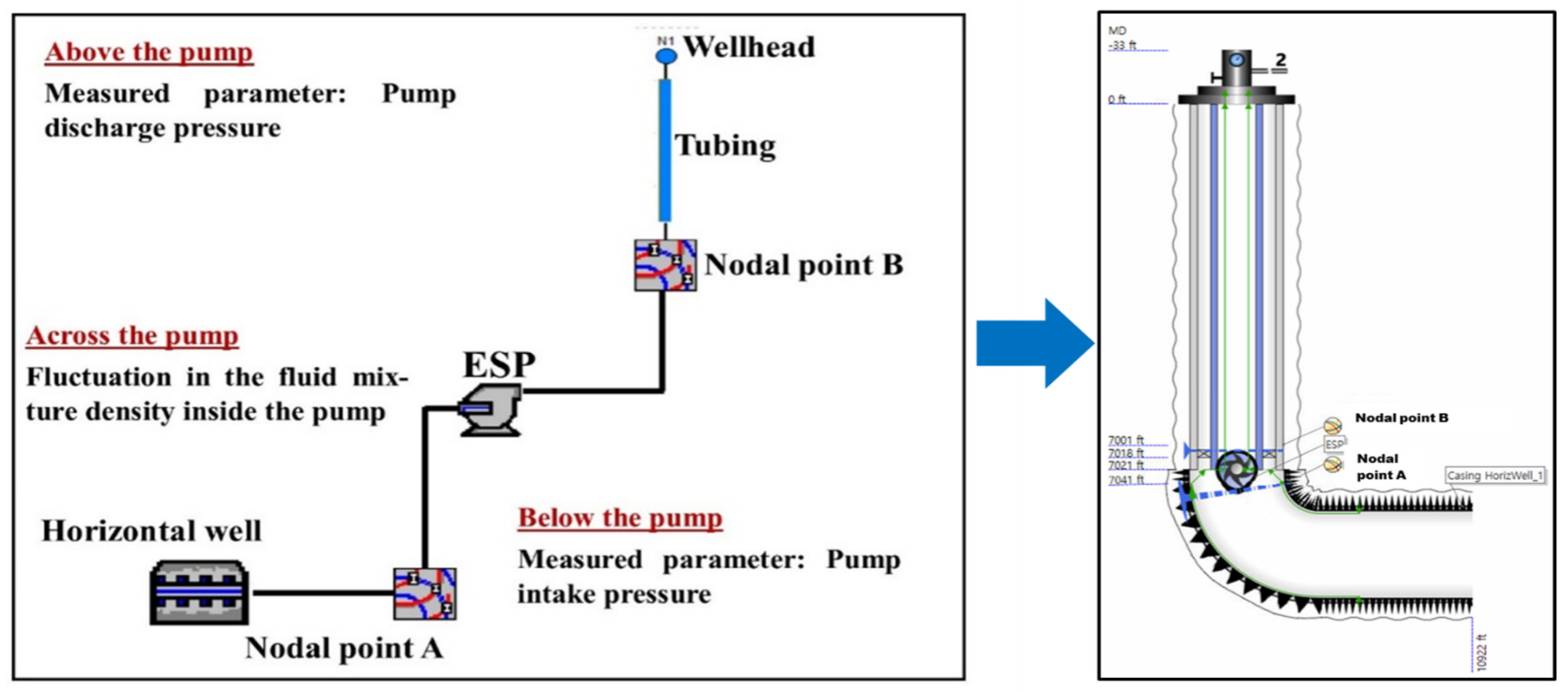
4.1. Model Formulation

An ESP converts fluid kinetic energy to hydraulic pressure when developing the required differential pressure. Performance is maximal when an ESP manages an incompressible fluid (e.g., water). Liquid with a density similar to water enhances pump performance; thus, fluid density directly affects ESP performance. Any density variation significantly affects the PIP and Pd. In practice, the fluid density significantly changes during oil production when the gas volume fraction (GVF) at the pump intake exceeds the design parameters. Pump operation fails; oil movement from the bottom hole to the surface decreases sharply, then stops [34]. To clarify the effect of free gas on ESP performance, an ESP well was divided into three compartments: from the pump discharge point to the wellhead, across the pump, and from the sand face to the ESP intake (Figure 1). The variation in each compartment was evaluated as the change in fluid density when the GVF increased. Awaid et al. [25] showed that a variation in Pd reflected a change in the upper ESP (Equation (1)), for example, at nodal point B of Figure 1. Equation (2) shows that differential pressure fluctuation across the pump can be affected by variations in fluid mixture density under identical pump head conditions; variations in $\mathrm{PIP}$ indicate events that occur below the pump (Equation (3)). The combination of these parameters defines the condition of the ESP well.

$${\mathrm{P}}_{\mathrm{disch}.}={\mathrm{P}}_{\mathrm{wh}}+\Delta {\mathrm{P}}_{\mathrm{garv}.}+\Delta {\mathrm{P}}_{\mathrm{fric}.}$$

(1)

$$\Delta {\mathrm{P}}_{\mathrm{pump}}=\mathrm{H}\times {\mathsf{\rho }}_{\mathrm{mix}}$$

(2)

$$\mathrm{PIP}={ \mathrm{P}}_{\mathrm{bh}}-\left(\Delta {\mathrm{P}}_{\mathrm{garv}.}+\Delta {\mathrm{P}}_{\mathrm{fric}.}\right)$$

(3)

where ${\mathrm{P}}_{\mathrm{disch}.}$ (psi) and $\mathrm{PIP}$ (psi) are defined above, ${\mathrm{P}}_{\mathrm{wh}} \mathrm{is}$ the wellhead pressure (psi), ${\mathrm{P}}_{\mathrm{bh}}$ is $\mathrm{the}$ bottom hole pressure, $\Delta {\mathrm{P}}_{\mathrm{garv}.}$ is $\mathrm{the}$ pressure loss related to gravity (psi), $\Delta {\mathrm{P}}_{\mathrm{fric}.} \mathrm{is} \mathrm{the}$ pressure loss related to friction, $\Delta {\mathrm{P}}_{\mathrm{pump}}$ (psi) is the differential pressure between ${\mathrm{P}}_{\mathrm{disch}.}$ and $\mathrm{PIP}$ (psi), $\mathrm{H} \mathrm{is} \mathrm{the}$ pumping head (ft), and ${\mathsf{\rho }}_{\mathrm{mix}}$ is the density of the fluid mixture (lb/ft³).

4.2. The Homogenous Model

The fluid densities at various GVFs were calculated using a homogenous model. The two-phase mixture (liquid and gas) was treated as a homogenous fluid [35]. The total mixture flow rate ${\mathrm{Q}}_{\mathrm{m}}$ is calculated as the sum of the in situ liquid (oil and water) flow rate ${\mathrm{Q}}_{\mathrm{l}}$ and the gas flow rate ${\mathrm{Q}}_{\mathrm{g}}$ (Equation (4)):

$${\mathrm{Q}}_{\mathrm{m}}={\mathrm{Q}}_{\mathrm{l}}+{\mathrm{Q}}_{\mathrm{g}}$$

(4)

Pessoa and Prado [35] showed that the pumping head under two-phase flow (${\mathrm{H}}_{\mathrm{tp}}$) could be expressed by multiplying the head of the single liquid phase (${\mathrm{H}}_{\mathrm{l}}$) and the degradation factor (the two-phase specific gravity, ${\mathrm{SG}}_{\mathrm{m}}$) for each individual GVF. Hence, ESP head degradation is given by Equation (8):

$${\mathsf{\lambda }}_{\mathrm{g}}={\mathrm{Q}}_{\mathrm{g}}/{\mathrm{Q}}_{\mathrm{m}}$$

(5)

$${\mathsf{\rho }}_{\mathrm{m}}={\mathsf{\lambda }}_{\mathrm{g}}{\mathsf{\rho }}_{\mathrm{g}}+\left[1-{\mathsf{\lambda }}_{\mathrm{g}}\right]{\mathsf{\rho }}_{\mathrm{l}}$$

(6)

$${\mathrm{SG}}_{\mathrm{m}}={\mathsf{\rho }}_{\mathrm{m}}/{\mathsf{\rho }}_{\mathrm{l}}$$

(7)

$${\mathrm{H}}_{\mathrm{tp}}={\mathrm{SG}}_{\mathrm{m}}{\mathrm{H}}_{\mathrm{l}}$$

(8)

where the new abbreviations are ${\mathsf{\rho }}_{\mathrm{l}}$ for the liquid density, ${\mathsf{\rho }}_{\mathrm{g}}$ for the gas density, and ${\mathsf{\lambda }}_{\mathrm{g}}$ for the GVF.

4.3. Nodal Analysis Simulation

Nodal analysis can be used to increase oil and gas well production by determining an optimal flow rate, identifying problems, and optimizing artificial lifting. A point of interest in the production system serves as a node; this is an intersection point of the inflow and outflow performance curves. Bruijnen [33] found that a combination of pump intake and discharge node data, as well as downhole pressure information, could be used to analyze ESP performance. The inflow and outflow curves are governed by Equations (9) and (10), respectively, when the intake pressure node serves as the nodal point (A in Figure 1).

$${\mathrm{I}}_{\mathrm{IPR}}=\mathrm{PIP}$$

(9)

$${\mathrm{V}}_{\mathrm{VLP}}-{\mathrm{E}}_{\mathrm{ESP}}=\mathrm{PIP}$$

(10)

The inflow and outflow curves are governed by Equations (11) and (12), respectively, when the discharge node serves as the nodal point (B in Figure 1).

$${\mathrm{I}}_{\mathrm{IPR}}+{\mathrm{E}}_{\mathrm{ESP}}={\mathrm{P}}_{\mathrm{d}}$$

(11)

$${\mathrm{V}}_{\mathrm{VLP}}={\mathrm{P}}_{\mathrm{d}}$$

(12)

where ${\mathrm{I}}_{\mathrm{IPR}}$ is the inflow performance relationship, ${\mathrm{E}}_{\mathrm{ESP}}$ is the ESP performance, ${\mathrm{V}}_{\mathrm{VLP}}$ is the vertical (tubing) lift performance, and PIP and Pd are defined above. We simulated this approach using Schlumberger PIPESIM software (version 2017.01); we employed nodal points A and B as defined above. To generalize the model, we evaluated different types of wells. For example, an ESP deployed in a dead well was used to stimulate production; an ESP installed in a naturally flowing well served to increase production. We considered both single-phase and multiphase conditions inside the pump. Using the homogenous model, we calculated the $\Delta {\mathrm{P}}_{\mathrm{pump}}$ at various GVF conditions. The PIP was estimated using nodal point A. The Pd was evaluated at nodal point B. Again, we set threshold ranges for normal operation by reference to field data; any point outside a range reflected an abnormality. For example, ESP operation was considered abnormal when the PIP deviation caused by gas slugging exceeded 5% in the Mangala oil field [27]. Dowling [34] reported that a PIP deviation > 3% indicated gas locking. Thus, we considered that PIP deviations $\pm$5% were normal, implying that the ESP operated under maximum production conditions (Q_max) when PIP fell by 5% from the design value; conversely, the ESP worked under the minimum operating conditions when the PIP increased by 5% of the design value—any greater deviation indicated an abnormality. In detail:

Step 1 (nodal analysis in the absence of the ESP): Nodal analysis proceeded under natural flow conditions prior to ESP installation; we estimated the bottomhole pressure (BHP) and production rate (Q_N) for a well exhibiting natural flow (Figure 2a) and the BHP for a dead well (Figure 2b).

Step 2 (nodal analysis in the presence of an ESP): The ESP was installed, and nodal analysis proceeded at the intake node (nodal point A, Figure 1). We recorded the operating ESP PIP_a and production rate (Q_a) under the design conditions (Figure 3a).

Step 3: We calculated the PIP_min (PIP_min = PIP_a + 0.05 PIP_a) and PIP_max (PIP_max = PIP_a − 0.05 PIP_a) and projected these onto Figure 3a to compute Q_min and Q_max (Figure 3b).

Step 4: We performed nodal analysis at the ESP discharge point (nodal point B, Figure 1) and estimated the discharge pressure of the operating pump (Pda) (Figure 4a).

Step 5: We plotted Q_min and Q_max (estimated in step 3) to compute Pd_min and Pd_max for the ESP discharge point (Figure 4b).

Moreover, based on Equations (9) and (10), a conceptual graph showing the variation in the tubing performance (TPR) curve was developed by reference to the ESP operating conditions. In Figure 5a–d, the TPR-ESP curve adequately represents the ESP tubing performance. As shown in Figure 5a–d, PIPa falls when the ESP is installed as designed. However, the ESP performance falls as the gas fraction increases inside the pump; the TPR-ESP curve is thus shifted upward until the ESP shuts down. Therefore, the PIP increases, and the oil production rate (${\mathrm{Q}}_{\mathrm{o}}$) decreases, compared with the design parameters.

Using Equations (11) and (12), a conceptual graph showing IPR curve variation was drawn to reflect production well status (ESP shutdown, normal ESP operation, and abnormal ESP operation) at the ESP discharge node (point B of Figure 1). The ESP performance curve is added to the IPR curve to generate the IPR + ESP curve (Equation (11)); this adequately represents the inflow performance of the ESP. As shown in Figure 6a–d, when an ESP is normally installed (i.e., under the design conditions), normal ESP operation increases the ${\mathrm{P}}_{\mathrm{d}}$ and ${\mathrm{Q}}_{\mathrm{o}}$, compared with abnormal ESP operation or ESP shutdown. Reduced ESP performance shifts the IPR curve downward, thereby reducing ${\mathrm{Q}}_{\mathrm{o}}$ and ${\mathrm{P}}_{\mathrm{d}}$.

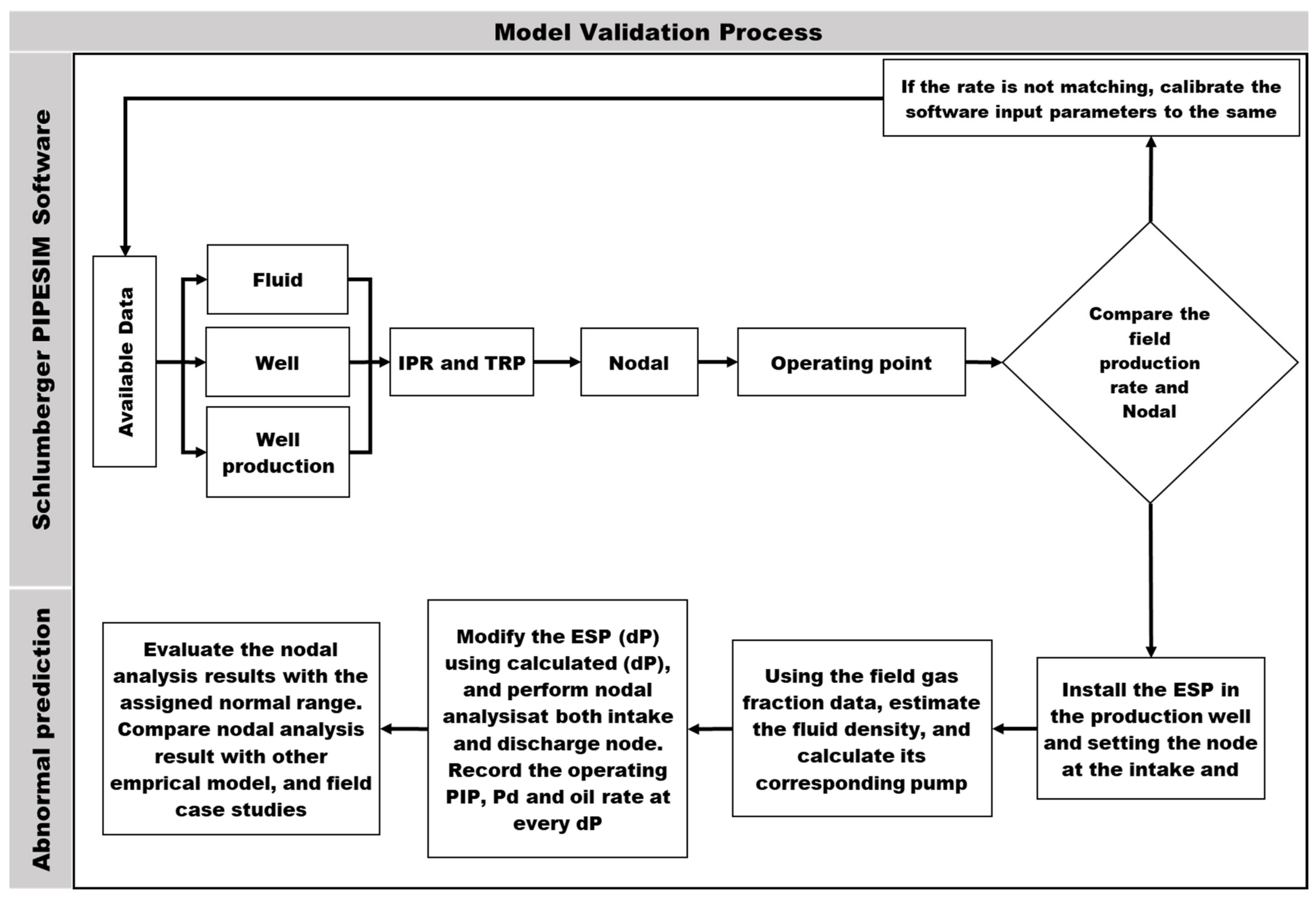
4.4. Model Validation and Interpretation

To evaluate the model’s utility, we used Delaware Basin oil well data to validate and calibrate the model under field conditions. We used the Schlumberger PIPESIM software (version 2017.01) to build a horizontal well model, then calibrated the model using field data, as shown in Figure 7. A horizontal oil well was considered as a test example.

Table 2. Input data sets, field example oil well.

Parameter
Reservoir pressure (psia)	3378.93
Reservoir temperature (F)	206
Payzone thickness (ft)	68
Horizontal distance (ft)	3901
Well permeability, (kx, ky, kz, respectively) (md)	0.05, 0.05, 0.05
Water cut (%)	92.9
Gas oil ratio, GOR (SCF/STB)	2218
Gas SG	0.65
API	42.98
Well measured depth (MD) (ft)	12,216
Tubing measured depth (MD) (ft)	7021
Tubing ID (in)	2.785
Oil production rate (STB/d)	430

summarizes the well, reservoir, fluid, and production data used in this model. The IPR curve was developed using the pseudo-steady state gas equation established by Babu and Odeh [36]. The pressure drop in the tubing was estimated by employing the Hagedorn and Brown correlation for vertical sections and the Beggs and Brill correlation for horizontal sections [37,38]. Thereby, the model estimated an approximate oil production rate of 430.3 STB/d. Less than 0.07% relative error was calculated compared to the field production rate.

After that, ESP equipment optimized for wells of various types was selected during nodal analysis. Then, the GVFs were increased from 0.03 to 0.99 at a fixed gas–oil ratio (GOR) and water cut (W_cut); the model was tested under multiphase conditions when GOR = 2218 SCF/STB and WC = 92.9% (real well data) and under single-phase conditions when GOR = 100 SCF/STB and W_cut = 0 (artificial data). We used the homogenous model to calculate the corresponding heads and PIP/Pd differential pressures at specified GVFs. Thus, we performed a sensitivity analysis of ESP behavior at the intake and discharge nodes using the calculated differential pressures when the GVF varied.

The Pd and PIP values at various GVFs were compared with the values of the specified, normal operating ranges (within ±5% of the design conditions). We developed a method predictive of ESP operation conditions, from normal to shutdown (

Table 3. Our scheme for prediction of ESP operation conditions.

Type of Production Well	ESP Operating Condition	At PIP Node	At Pd Node
Natural flowing well (or dead well)	Normal	PIPmax < PIPa < PIPmin	Pdmax > Pda > Pdmin
	The transition from normal to abnormal conditions (surging)	PIPa = PIPmin	Pda = Pdmin
	Abnormal operation	PIPa > PIPmin	Pda < Pdmin
	Gas locking (pump stopped); return to natural flow	PIPa = Pda = BHP	Pda = Pda = BHP

). The PIPs calculated at nodes were used to predict the critical gas fractions (${\lambda }_{\mathrm{c}}$ values) at which an ESP abnormality (surging) commenced. For example, Ref. [15] showed that abnormal ESP operation commenced when the Turpin correlation ∅_Turpin ≥ 1 (Table 1). Using this correlation, the $\mathrm{PIPs}$ appropriate for all pump conditions studied during nodal analysis were used to compute the corresponding critical gas fractions. We also employed the correlations established by Cirilo, Romero Dunbar, and Zhou (Table 1).

5. Results

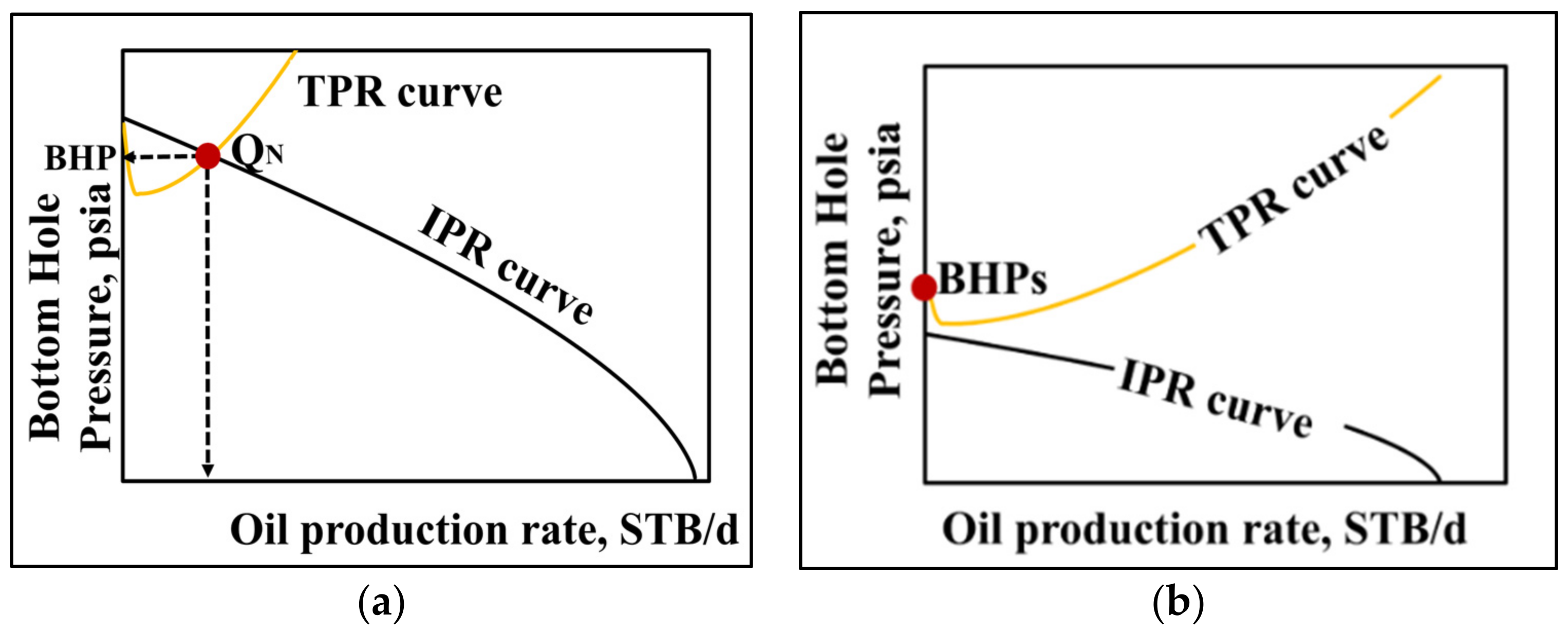
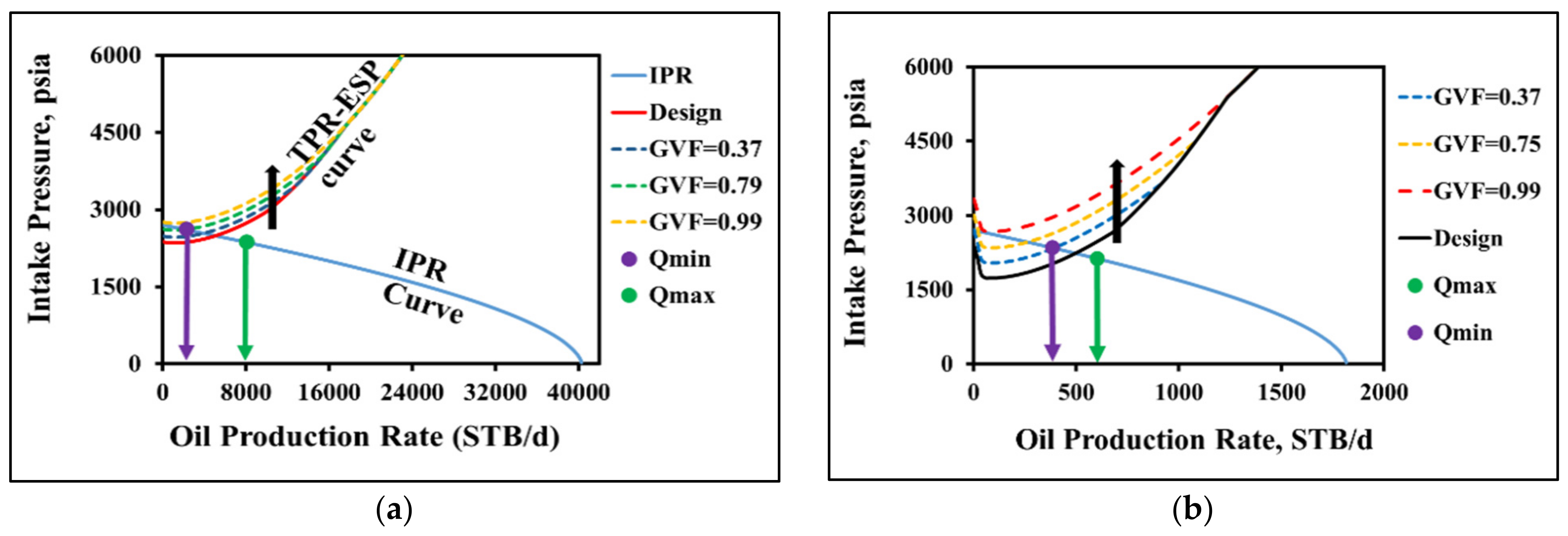
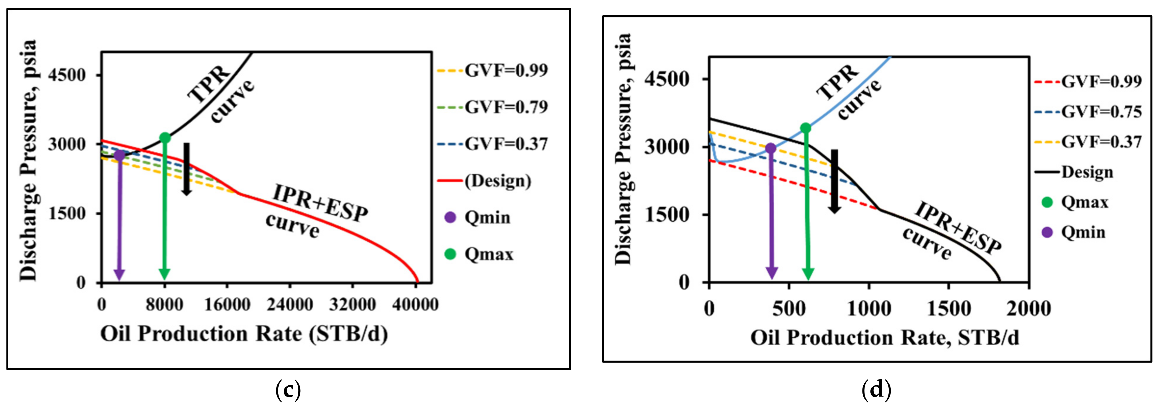
5.1. Results of Nodal Analysis Simulation

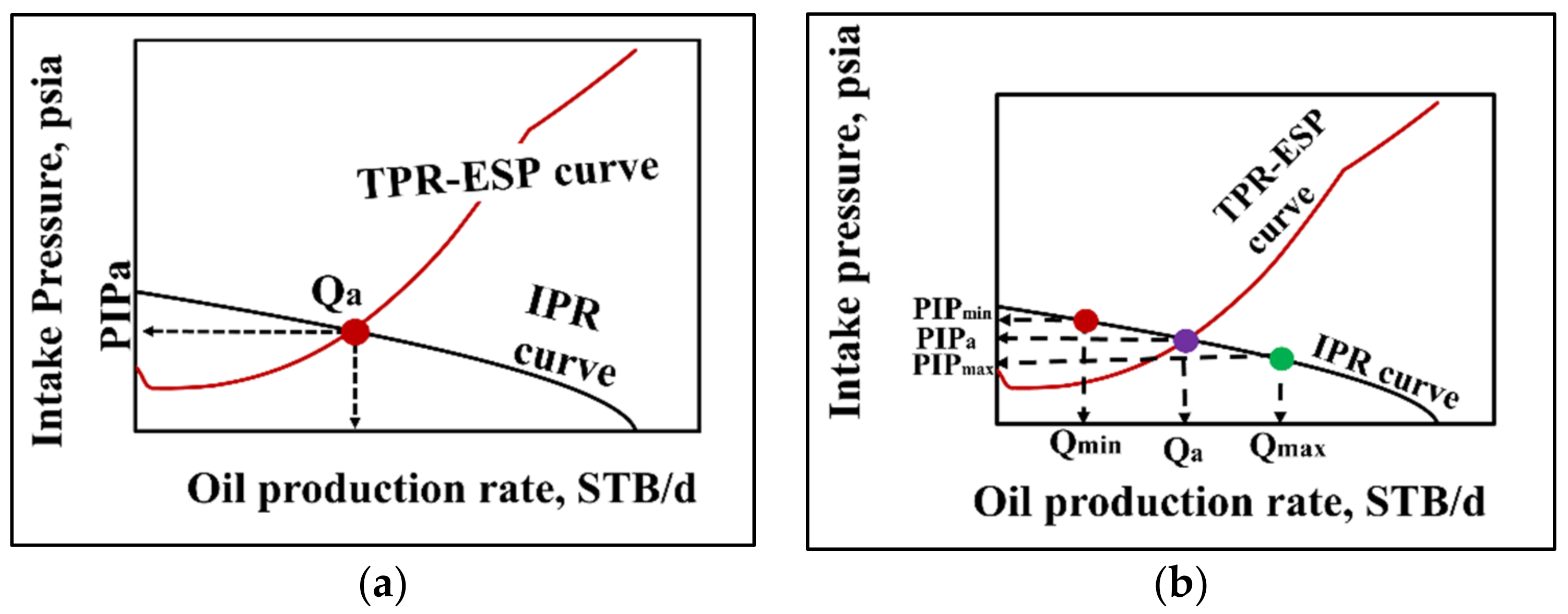
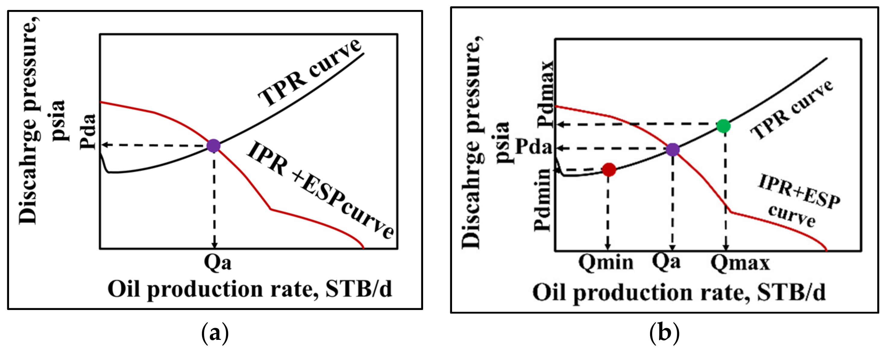
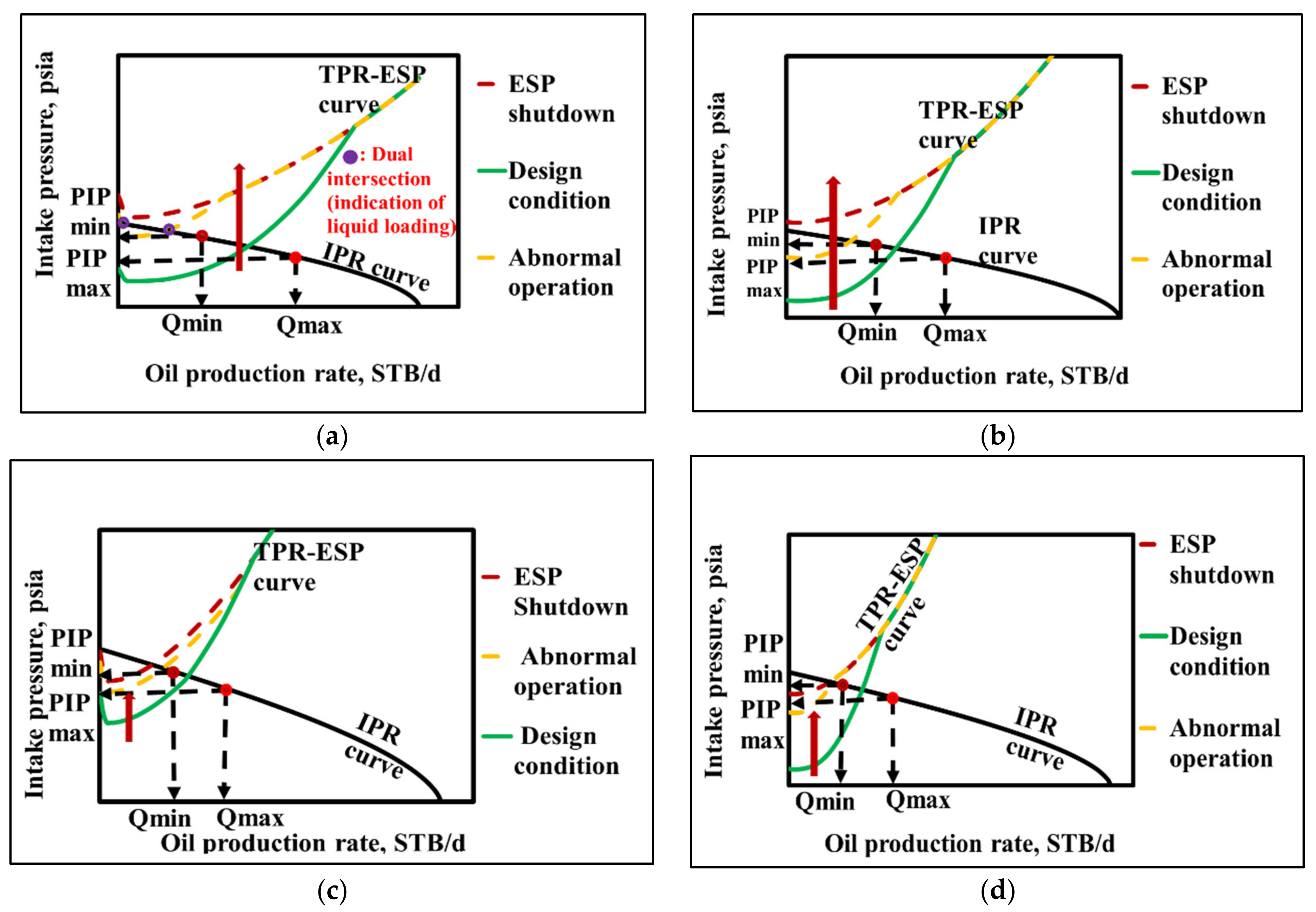
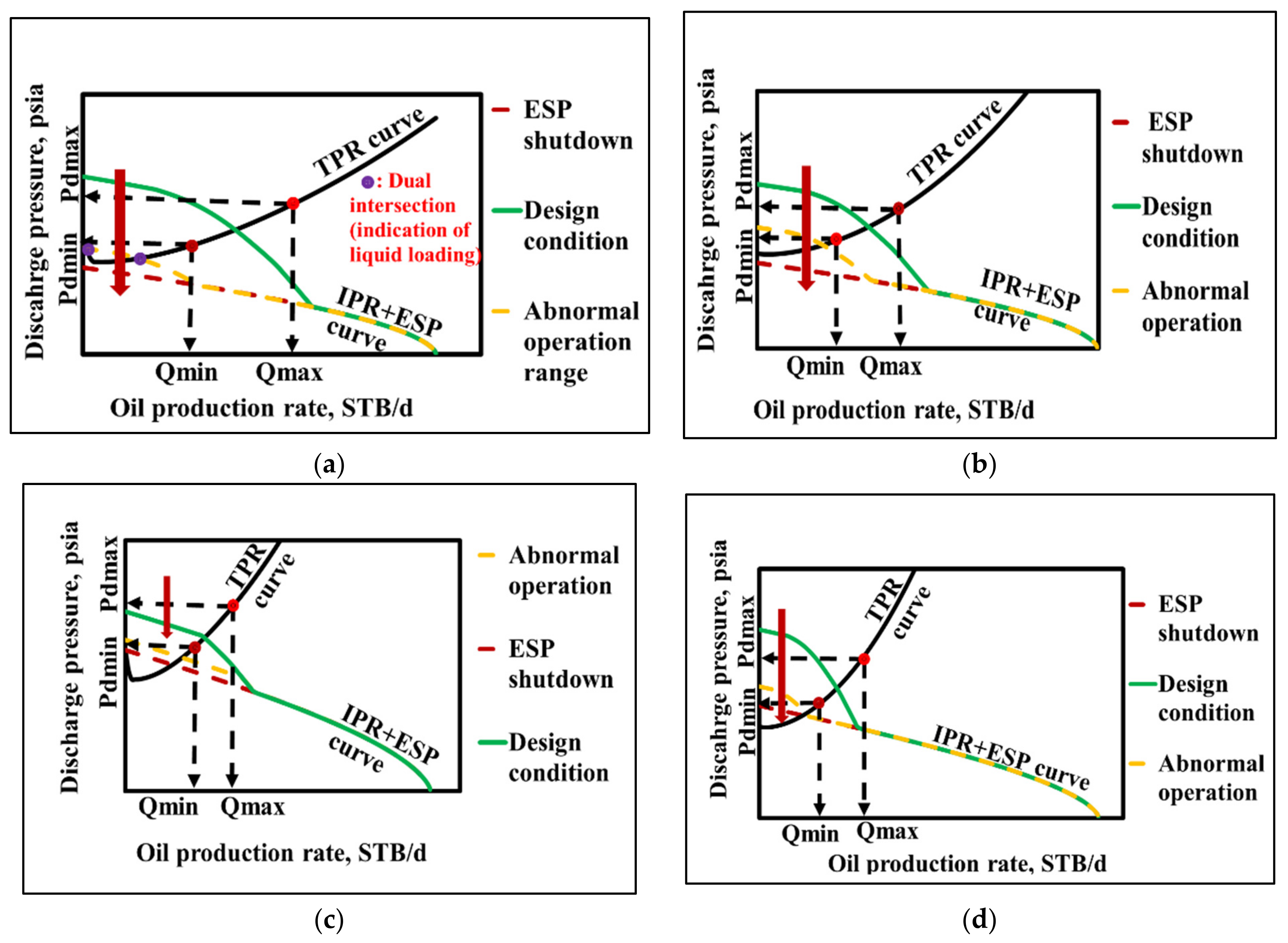
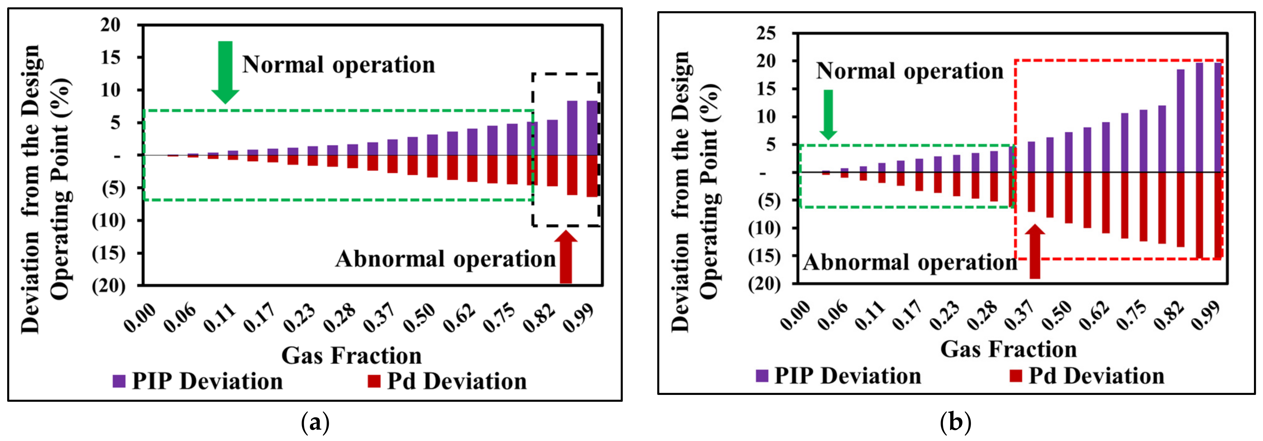
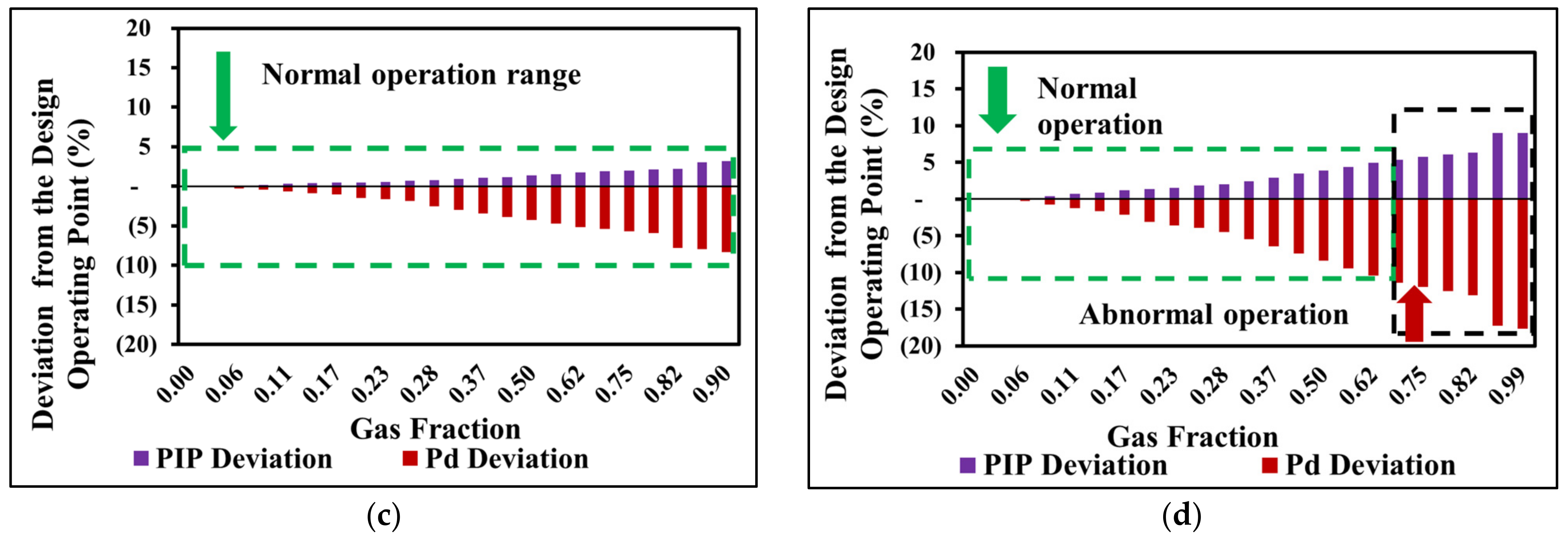
The effects of an increasing GVF on ESP performance were evaluated at both the intake node (nodal point A, Figure 1) and the discharge node (nodal point B, Figure 1). The intake node evaluation yielded the operating PIP given by the intersection of the TPR-ESP and IPR curves. Similarly, evaluation at the discharge node yielded the operating Pd given by the intersection of the TPR and IPR + ESP curves.

Case one shows the nodal analysis of GVF variation when an ESP is deployed in a dead well. Thus, the IPR and TPR-ESP curves do not intersect when GVF = 0.99 (the ESP is not operating). Figure 8a shows that the TPR-ESP curve moves upward when the GVF increases; Figure 8b shows that the operating intake nodal point is shifted to the left of the IPR curve, thereby increasing PIP and reducing Q_o. Similarly, Figure 8c shows that the IPR + ESP curve moves downward when the GVF increases; Figure 8d shows that the discharge nodal point shifts to the left of the minimum point on the TPR curve. Because of these changes, both P_d and Q_o decrease. The pressure difference ($\Delta {\mathrm{P}}_{\mathrm{pump}}$) between $PIP$ and $P_d$ gradually decreases as GVF increases. Thus, ESP performance and oil production both decrease.

Case two shows the nodal analysis of GVF changes when an ESP is deployed in a naturally flowing well; the TPR-ESP and IPR curves intersect when the GVF is 0.99, although the ESP is not operating. Similar to case one, an increase in the GVF degrades ESP performance, thereby increasing the TPR curve (Figure 9a,b) and decreasing the IPR curve (Figure 9a,c). Q_min develops at GVF = 0.69 for a multiphase well (Figure 9b,d). Thus, the ESP operation is abnormal when GVF exceeds 0.69. However, for a single-phase well, ESP operation is normal despite a GVF of 0.99 (Figure 9a,c) because all intersection points of the TPR and IPR curves are within the reference threshold normal ranges.

The changes in the TPR and IPR curves when the GVF increases can be interpreted over three phases:

Phase I: Stable ESP operation. In this phase, the TPR and IPR curves intersect within the normal operating ranges, irrespective of the ESP operating point. The intersections (TPR-ESP and IPR curves or IPR + ESP and TPR curves) are stabilized within the threshold, normal operating ranges. For example, at a fixed GOR = 100 SCF/STB and W_cut = 0, the intersection points remain in the normal ranges until GVF attains 0.79 (dead well, Figure 8a,c). When GOR = 2218 SCF/STB and W_cut = 92.9%, the intersection points remain in the normal ranges until GVF exceeds 0.37 (dead well, Figure 8b,d).

Phase II: Abnormal operation. The TPR and IPR curves intersect outside the normal threshold ranges during this phase. Despite the abnormality, ESP operation continues; the differential pressure becomes low. At a fixed GOR = 100 SCF/STB and a W_cut = 0, operation becomes abnormal when the GVF exceeds 0.79 (dead well, Figure 8a,c). When GOR = 2218 SCF/STB and W_cut = 92.9%, abnormal operation is observed when the GVF exceeds 0.37 (dead well, Figure 8b,d) or 0.69 (naturally flowing well, Figure 9b,d).

Phase III: The ESP is shut down, and the well operates under natural flow conditions. This phase comprises two parts, depending on the condition of the well prior to ESP installation. For a dead well, Phase III is associated with zero production. Conversely, when the well previously flowed naturally, it shifts to its natural operating point when this phase initiates. The measured PIP and ${\mathrm{P}}_{\mathrm{d}}$ are very similar to the operating bottomhole pressure of the (formerly) naturally flowing well; this is the ESP shutdown condition. When the ESP shuts down, the TPR-ESP and IPR + ESP curves coincide with the curves of the natural well (at a GVF = 0.99, Figure 8 and Figure 9).

5.2. ESP Operation as ${\mathrm{P}}_{\mathrm{disch}}$ and PIP Deviate

Awaid et al. [25] found that hydraulic parameters were critical when monitoring ESP operation under multiphase conditions. ${\mathrm{P}}_{\mathrm{d}}$ reflects the fluid properties in terms of tubing behavior and slugging effects; $\mathrm{PIP}$ reflects the fluid properties below the pump and the liquid level in the casing. It is important to understand that ${\mathrm{P}}_{\mathrm{disch}}$ and $\mathrm{PIP}$ vary according to the GVF; these deviations must be considered when analyzing ESP operation. Figure 10 shows these deviations when the GVF increases. The deviations are greater when an ESP operates under multiphase conditions; performance degradation is then high.

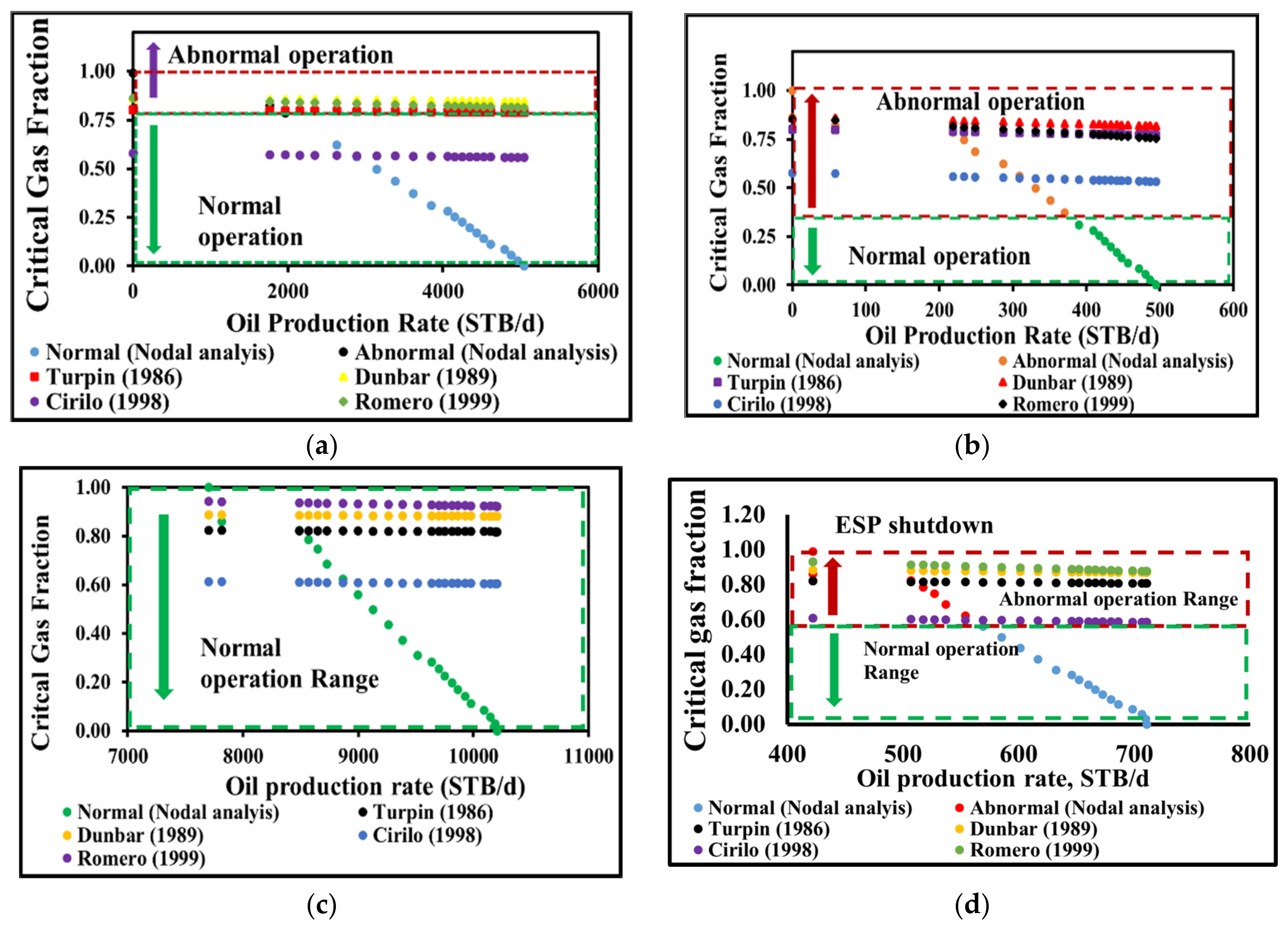
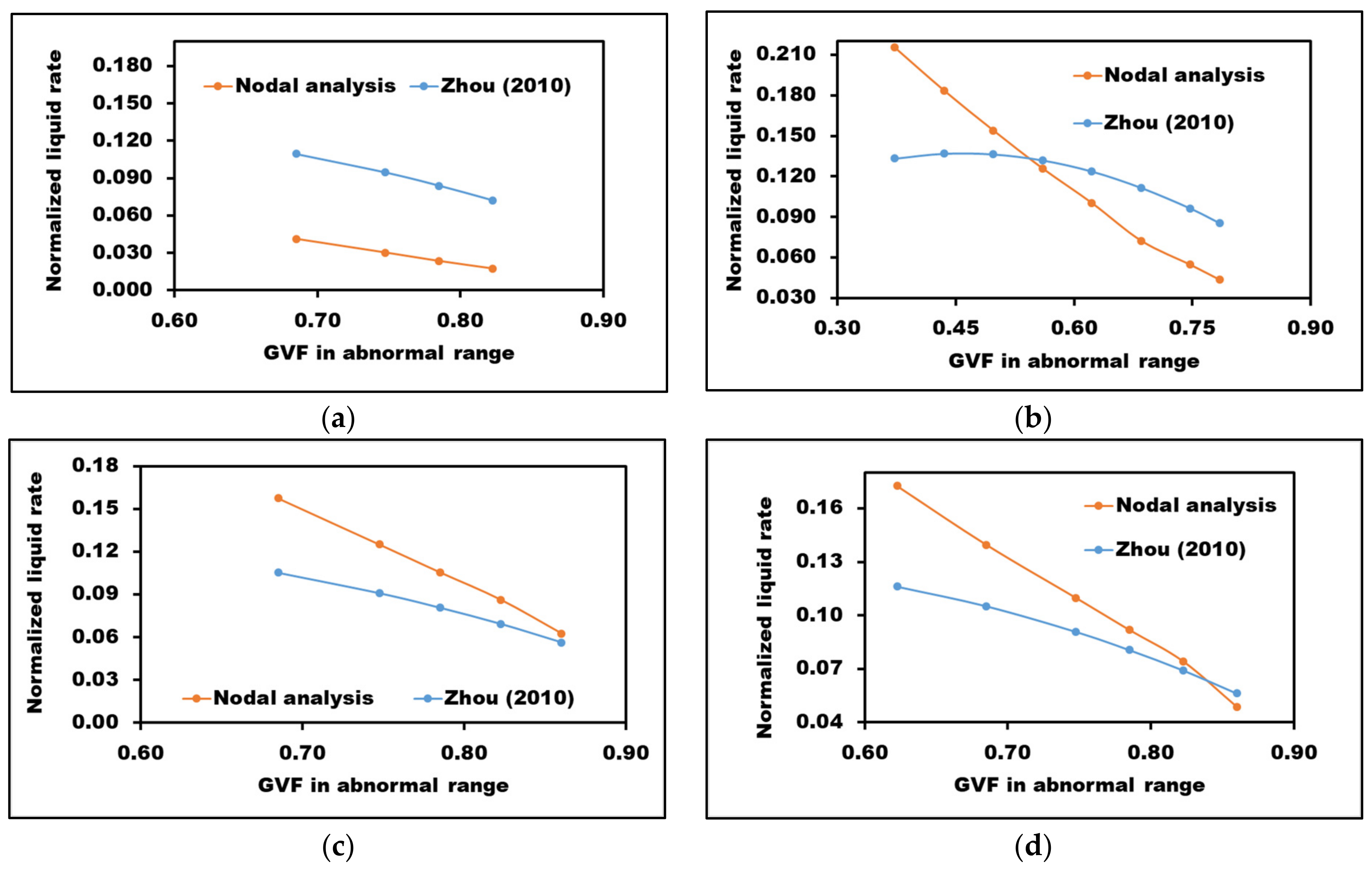
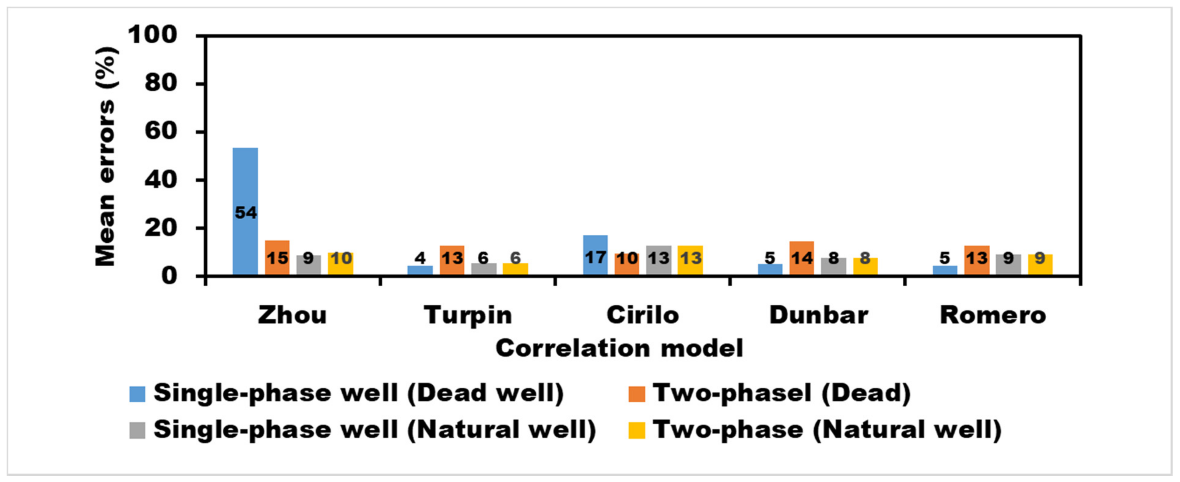
5.3. Comparison of Nodal Analysis and Surging Prediction Models

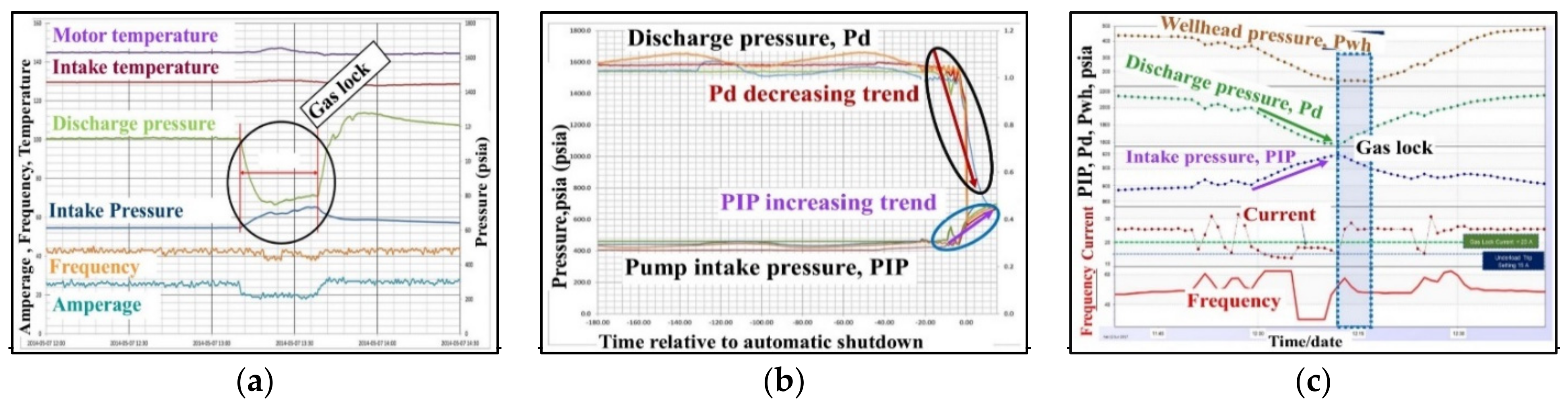
The operating PIPs recorded at every GVF during nodal analysis were used to compute the corresponding critical gas fractions using the models established by Cirilo [17], Romero [18], Dunbar [16], and Turpin (the correlation model) [15] (Table 1). Except for the Cirilo correlation, the correlations of the other models were consistent with the predictions afforded by nodal analysis (Figure 11).

The operating PIP and GVF from the nodal analysis were also used to calculate the corresponding normalized liquid rate using Zhou (the correlation model) [14] (Table 1). Both nodal analysis and Zhou normalized rate at different GVFs were compared, and the results showed a consistent trend (Figure 12). The normalized rate decreasing trend was observed when GVF increased, indicating the ESP abnormal condition (failed to pump the liquid at high GVF).

5.4. Changes in the PIP and ${\mathrm{P}}_{\mathrm{disch}.}$—A Field Example

A field example was used to evaluate the observed changes in PIP and Pd. Example 1 (Figure 13a) shows that the ESP was operating stably when a sudden gas increase occurred. This was followed by an abrupt increase in the PIP and a decrease in the Pd. The ESP was gas locked briefly but quickly resumed normal operation. A PIP increase and a Pd decrease normally signal a gas lock [34]. Example 2 (Figure 13b) illustrates automatic ESP shutdown when the differential pressure becomes zero. In this example, an increase of gas at the ESP intake caused the PIP to rise and the Pd to fall. The ESP operated at increasingly low production rates until the PIP and Pd attained the same values; the ESP automatically shut down. Example 3 (Figure 13c) shows the PIP and Pd variations caused by severe gas degradation. When the pump ingests substantial gas, ESP efficiency is reduced as the Pd falls and the PIP rises. These trends continue until the lift is insufficient and the ESP shuts down. The wellhead production rate becomes zero, as shown by the constant wellhead pressure [39]. These field examples show that our model will find practical applications.

5.5. Model Assessment

This section compares standard errors, normality, and homogeneity of the critical GVFs predicted using nodal analysis and the empirical models developed by Cirilo, Romero, Dunbar, and Turpin (the correlation model). The normalized liquid rate obtained from the nodal analysis was also compared with Zhou (2010) (the empirical model). The average deviation error was calculated based on the nodal analysis for each model; thus, 4–13%, 5–13%, 5–14%, 13–17%, and 9–54% increases were observed in the Turpin (1986), Romero (1999), Dunbar (1989), Cirilo (1998), and Zhou (2010) models, respectively (Figure 14). Better result matching was observed at the GVF above 0.8; unexpectedly high standard deviation error in the Zhou model resulted from the low production rate associated with the dead well conditions. Since the Zhou model relies on the pump design capacity, such as maximum flow rate, its prediction can be erroneous, especially in a low rate well. The Zhou model performs better at a high production rate well condition (for example, less than 10% average error was observed when ESP is operating in natural well condition). Other models are consistent, with less than 17% error in all well conditions. The Shapiro–Wilk normality test was performed at a 95% confidence level. Except for the Cirilo model, other correlations were normally distributed in the abnormal range predicted using the nodal analysis (

Table 4. Results of the Shapiro–Wilk normality test (critical GVF predicted in abnormal operating range).

Correlation	Case 1a		Case 1b		Case 2a		Case 2b
	W	p-Value	W	p-Value	W	p-Value	W	p-Value
Nodal analysis	0.969	0.700	0.963	0.700	0.986	0.985	0.986	0.985
Turpin (1986)	0.829	0.075	0.953	0.700	0.847	0.300	0.874	0.300
Cirilo (1998)	0.777	0.035	0.952	0.700	0.846	0.300	0.873	0.300
Dunbar(1989)	0.870	0.300	0.953	0.700	0.847	0.300	0.857	0.300
Romero (1999)	0.876	0.300	0.952	0.700	0.845	0.300	0.872	0.300

W: statistic test value, Case 1a: single-phase dead well, Case 1b: two-phase dead well, Case 2a: single-phase natural flowing well, and Case 2b: two-phase natural well. The significant p-values (<0.05) are shown in bold.

and

Table 5. Results of the Shapiro–Wilk normality test (normalized liquid rate calculated in abnormal operating range).

Correlation	Case 1a		Case 1b		Case 2a		Case 2b
	W	p-Value	W	p-Value	W	p-Value	W	p-Value
Nodal analysis	0.925	0.300	0.951	0.700	0.994	0.990	0.985	0.965
Zhou (2010)	0.913	0.300	0.852	0.300	0.995	0.700	0.982	0.965

W: statistic test value, Case 1a: single-phase dead well, Case 1b: two-phase dead well, Case 2a: single-phase natural flowing well, and Case 2b: two-phase natural well. The significant p-values (<0.05) are shown in bold.

). We performed a Chi-square test to evaluate the homogeneity of the results. It was found that the models’ results are homogenous (

Table 6. Results of the Chi-square homogeneity test (both normalized liquid rate and critical GVF obtained in the abnormal operating range).

Correlation	Case 1a		Case 1b		Case 2a		Case 2b
	W	p-Value	W	p-Value	W	p-Value	W	p-Value
Turpin (1986)	0.03	1.00	0.11	1.00	0.05	1.00	0.05	1.00
Cirilo (1998)	0.02	1.00	0.09	1.00	0.04	1.00	0.04	1.00
Dunbar (1989)	0.03	1.00	0.11	1.00	0.06	1.00	0.06	1.00
Romero (1999)	0.02	1.00	0.14	1.00	0.05	1.00	0.05	1.00
Zhou (2010)	0.02	1.00	0.05	1.00	0.01	1.00	0.01	1.00

W: statistic test value, Case 1a: single-phase dead well, Case 1b: two-phase dead well, Case 2a: single-phase natural flowing well, and Case 2b: two-phase natural well. The significant p-values (<0.05) are shown in bold.

).

6. Conclusions and Recommendation

We used nodal analysis to predict abnormal ESP operation when free gas at the ESP intake suddenly increases. The model was validated using various multiphase surging models (developed using experimental results) and field data (where the gas lock problem was reported). Our conclusions are:

(1)

Nodal analysis precisely predicted ESP operating conditions by matching real-time downhole and surface sensor data trends. Nodal analysis can be used for real-time monitoring of ESP wells.

(2)

Nodal analysis can be used to manage future ESP wells; the normal operating ranges are based on the natural conditions of the well. Such proactive planning prevents uncertainties that might otherwise arise when an ESP is installed.

(3)

The nodal analysis allows quick diagnosis and interpretation of downhole sensor data, facilitating rapid responses to ESP conditions that might otherwise damage the pump.

(4)

We add to the current body of ESP well-monitoring knowledge.

This work is novel in that we introduce (and define) reference, threshold, and normal operating ranges for the several distinct phases of ESP operation: the stable phase (when the operating points decrease in such ranges); the abnormal condition (a point outside of the normal range); and ESP shutdown (before an ESP returns to natural flow status). Existing methods consider only ESP failure.

Despite the utility of the model, care is needed. The PIP, Pd, and flow rate can be changed due to the various production conditions (for example, a decrease in reservoir pressure, a decrease or increase in the productivity index). The reference threshold normal ranges must then be updated. The model will be particularly useful in oilfields where free gas is the major cause of potential ESP failure. Further studies are needed to determine whether the proposed model can be used not only in the high GOR condition but also to the other ESP failure conditions.

References

1. Peng, L.; Han, G.; Sui, X.; Pagou, A.L.; Zhu, L.; Shu, J. Predictive approach to perform fault detection in electrical submersible pump systems. ACS Omega 2021, 6, 8104–8111. [Google Scholar] [CrossRef] [PubMed]
2. Vald, J.P.; Becerra, D.; Rozo, D.; Cediel, A.; Torres, F.; Asuaje, M.; Sim, U. Comparative analysis of an electrical submersible pump’ s performance handling viscous Newtonian and non-Newtonian fluids through experimental and CFD approaches. J. Pet. Sci. Eng. 2020, 187, 106749. [Google Scholar] [CrossRef]
3. Ofuchi, E.M.; Stel, H.; Vieira, T.S.; Ponce, F.J.; Chiva, S.; Morales, R.E.M. Study of the effect of viscosity on the head and fl ow rate degradation in different multistage electric submersible pumps using dimensional analysis. J. Pet. Sci. Eng. 2017, 156, 442–450. [Google Scholar] [CrossRef]
4. Ali, A.; Yuan, J.; Deng, F.; Wang, B.; Liu, L.; Si, Q.; Buttar, N.A. Research progress and prospects of multi-stage centrifugal pump capability for handling gas-liquid multiphase flow: Comparison and empirical model validation. Energies 2021, 14, 896. [Google Scholar] [CrossRef]
5. Takacs, G. Submersible Electrical Pumps Manual: Design, Operations and Maintenance, 2nd ed.; Elsevier: Amsterdam, The Netherlands, 2018; ISBN 9780128145708. [Google Scholar]
6. Nguyen, T.C.; Pande, S.; Bui, D.; Al-Safran, E.; Nguyen, H.V. Pressure dependent permeability: Unconventional approach on well performance. J. Pet. Sci. Eng. 2020, 193, 107358. [Google Scholar] [CrossRef]
7. Manshad, A.K.; Dastgerdi, M.E.; Ali, J.A.; Mafakheri, N.; Keshavarz, A.; Iglauer, S.; Mohammadi, A.H. Economic and productivity evaluation of different horizontal drilling scenarios: Middle East oil fields as case study. J. Pet. Explor. Prod. Technol. 2019, 9, 2449–2460. [Google Scholar] [CrossRef] [Green Version]
8. Clegg, J.D. Operations Petroleum Engineering Production Operations Engineering; Society of Petroleum Engineers: Richardson, TX, USA, 2007; Volume IV, ISBN 978-1-55563-118-5. [Google Scholar]
9. Kolawole, O.; Gamadi, T.D.; Bullard, D. Artificial lift system applications in tight formations: The state of knowledge. SPE Prod. Oper. 2020, 35, 422–434. [Google Scholar] [CrossRef]
10. Stel, H.; Sirino, T.; Ponce, F.J.; Chiva, S.; Morales, R.E.M. Numerical investigation of the flow in a multistage electric submersible pump. J. Pet. Sci. Eng. 2015, 136, 41–54. [Google Scholar] [CrossRef]
11. Zhu, J.; Guo, X.; Liang, F.; Zhang, H.Q. Experimental study and mechanistic modeling of pressure surging in electrical submersible pump. J. Nat. Gas Sci. Eng. 2017, 45, 625–636. [Google Scholar] [CrossRef]
12. Lea, J.F.; Bearden, J.L. Effect of Gaseous Fluids on Submersible Pump Performance. JPT J. Pet. Technol. 1982, 34, 2922–2930. [Google Scholar] [CrossRef]
13. Gamboa, J.; Prado, M. Review of electrical-submersible-pump surging correlation and models. SPE Prod. Oper. 2011, 26, 314–324. [Google Scholar] [CrossRef]
14. Zhou, D.; Sachdeva, R. Simple model of electric submersible pump in gassy well. J. Pet. Sci. Eng. 2010, 70, 204–213. [Google Scholar] [CrossRef]
15. Turpin, J.L.; Lea, J.F.; Bearden, J.L. Gas-liquid flow through centrifugal pumps—correlation of data. In Proceedings of the 3rd International Pump Symposium, Texas A&M University, College Station, TX, USA, 1 May 1986. [Google Scholar]
16. Pessoa, R.; Prado, M. Experimental investigation of two-phase flow performance of electrical submersible pump stages. In Proceedings of the SPE Annual Technical Conference and Exhibition, New Orleans, LA, USA, 30 September–3 October 2001. [Google Scholar] [CrossRef]
17. Cirilo, R. Air-water Flow Through Electric Submersible Pumps; Artificial Lift Projects Research Report; University of Tulsa: Tulsa, OK, USA, 1998. [Google Scholar]
18. Romero, M. An Evaluation of An Electrical Submersible Pumping System for High Gor Wells. Master’s Thesis, University of Tulsa, Tulsa, OK, USA, 1999. [Google Scholar]
19. Duran, J.; Prado, M. ESP Stages air-water two-phase performance-modeling and experimental data. SPE J. 2003, 13, 196105718. [Google Scholar]
20. Zhu, J.; Zhang, J.; Cao, G.; Zhao, Q.; Peng, J.; Zhu, H.; Zhang, H.Q. Modeling flow pattern transitions in electrical submersible pump under gassy flow conditions. J. Pet. Sci. Eng. 2019, 180, 471–484. [Google Scholar] [CrossRef]
21. Zhu, J.; Zhang, H.Q. A review of experiments and modeling of gas-liquid flow in electrical submersible pumps. Energies 2018, 11, 180. [Google Scholar] [CrossRef] [Green Version]
22. Diaz, N.I.C. Effects of Sand on the Components and Performance of Electrical Submersible Pumps. Master’s Thesis, Texas A&M University, College Station, TX, USA, 2012. [Google Scholar]
23. Jansen van Rensburg, N. Usage of artificial intelligence to reduce operational disruptions of ESPs by implementing predictive maintenance. In Proceedings of the Abu Dhabi International Petroleum Exhibition & Conference, Abu Dhabi, United Arab Emirates, 12–15 November 2018. [Google Scholar] [CrossRef]
24. Oyewole, P. Application of real-time ESP data processing and interpretation in Permian basin “brownfield” operation. In Proceedings of the International Petroleum Technology Conference, Doha, Qatar, 21–23 November 2005. [Google Scholar] [CrossRef]
25. Awaid, A.; Al-Muqbali, H.; Al-Bimani, A.; Al-Yazeedi, Z.; Al-Sukaity, H.; Al-Harthy, K.; Baillie, A. ESP well surveillance using pattern recognition analysis, oil wells, Petroleum Development Oman. In Proceedings of the International Petroleum Technology Conference, Doha, Qatar, 19–22 January 2014. [Google Scholar] [CrossRef]
26. Al-sadah, H.; Khamseen, M.A.; Al-ghamdi, A.; Fardan, A.; Aramco, S. Proactive utilization of ESP performance monitoring to enhance productivity. In Proceedings of the SPE Middle East Oil and Gas Show and Conference, Manama, Bahrain, 18–21 March 2019. [Google Scholar] [CrossRef]
27. Agrawal, N.; Chapman, T.; Baid, R.; Singh, R.K.; Shrivastava, S.; Kushwaha, M.K. ESP performance monitoring and diagnostics for production optimization in polymer flooding: A case study of Mangala field. In Proceedings of the SPE Oil and Gas India Conference and Exhibition, Mumbai, India, 9–11 April 2019. [Google Scholar] [CrossRef]
28. Nunez, W.; Del Pino, J.; Gomez, S.; Rosales, D.; Puentes, J.; Rivera, H. Electric submersible pump troubleshooting guide, an effective way to improve system performance and reduce avoidable system failures. In Proceedings of the SPE Latin American and Caribbean Petroleum Engineering Conference, Vitrul, 20 July 2020. [Google Scholar] [CrossRef]
29. Barrios Castellanos, M.; Serpa, A.L.; Biazussi, J.L.; Monte Verde, W.; do Socorro Dias Arrifano Sassim, N. Fault identification using a chain of decision trees in an electrical submersible pump operating in a liquid-gas flow. J. Pet. Sci. Eng. 2020, 184, 106490. [Google Scholar] [CrossRef]
30. Liang, X.; Ghoreishi, O.; Xu, W. Downhole tool design for conditional monitoring of electricalsubmersible motors in oil field facilities. IEEE Trans. Ind. Appl. 2017, 53, 3164–3174. [Google Scholar] [CrossRef]
31. Li, L.; Hua, C.; Xu, X. Condition monitoring and fault diagnosis of electric submersible pump based on wellhead electrical parameters and production parameters. Syst. Sci. Control Eng. 2018, 6, 253–261. [Google Scholar] [CrossRef]
32. Fusiek, G.; Niewczas, P.; Judd, M.D. Towards the development of a downhole optical voltage sensor for monitoring electrical submersible pumps. Sens. Actuators A Phys. 2012, 184, 173–181. [Google Scholar] [CrossRef]
33. Bruijnen, P.M. Nodal analysis by use of ESP intake and discharge pressure gauges. SPE Prod. Oper. 2016, 31, 76–84. [Google Scholar] [CrossRef]
34. Dowling, M.A. You don’ t know pumps: Myths and truths about ESP operation in high-gas environments. In Proceedings of the SPE Electric Submersible Pump Symposium, The Woodlands, TX, UAS, 9–11 April 2019. [Google Scholar] [CrossRef]
35. Pessoa, R.; Prado, M. Two-phase flow performance for electrical submersible pump stages. SPE Prod. Facil. 2003, 18, 13–27. [Google Scholar] [CrossRef]
36. Babu, D.K.; Odeh, A.S. Productivity of a horizontal well. SPE Res. Eng. 1988, 4, 417–421. [Google Scholar] [CrossRef]
37. Beggs, H.D.; Brill, J.R. Study of Two-Phase Flow in Inclined Pipes. JPT J. Pet. Technol. 1973, 25, 607–617. [Google Scholar] [CrossRef]
38. Hagedorn, A.R.; Brown, K.E. Experimental Study of Pressure Gradients Occurring During Continuous Two-Phase Flow in Small-Diameter Vertical Conduits. J. Pet. Technol. 1965, 17, 475–484. [Google Scholar] [CrossRef]
39. Camilleri, L.A.; Gong, H.; Al-Maqsseed, N.H.; Al-Jazzaf, A.M. Tuning VSDs in ESP wells to optimize oil production—case studies. In Proceedings of the SPE Artificial Lift Conference and Exhibition—Americas, The Woodlands, TX, USA, 28–30 August 2018. [Google Scholar] [CrossRef]
Figure 1. Nodal analysis simulation model. (Left) Schematic diagram of the ESP horizontal oil well components. (Right) Shows the model representation in Schlumberger PIPESIM software (version 2017.01), developed by Schlumberger, located in Houston, TX, USA.
Applsci 12 02825 g001
Figure 2. (a) Operating BHP for a naturally flowing well. (b) Static BHP for a dead well.
Applsci 12 02825 g002
Figure 3. ESP PIP operating threshold limits. (a) Design conditions. (b) Minimum and maximum normal operating threshold limits.
Applsci 12 02825 g003
Figure 4. Computation of the ESP (discharge pressure) operating threshold limit. (a) Design conditions. (b) Minimum and maximum normal operating threshold limits.
Applsci 12 02825 g004
Figure 5. Variations in TPR curves as ESP performance varies. (a) Multiphase flow (dead well), (b) single-phase flow (dead well), (c) multiphase flow (naturally flowing well), (d) single-phase flow (naturally flowing well). The TPR-ESP curve reflects the TPR of a well with an ESP when the nodal analysis is performed at the intake (nodal point A of Figure 1).
Applsci 12 02825 g005
Figure 6. IPR curve variations at various ESP performances. (a) Multiphase flow (a dead well); (b) single-phase flow (a dead well); (c) multiphase flow (a naturally flowing well); (d) single-phase flow (a naturally flowing well). The IPR + ESP curve adequately reproduces the IPR + ESP curve when the nodal analysis is focused on the discharge node (nodal point B of Figure 1).
Applsci 12 02825 g006
Figure 7. Model validation process.
Applsci 12 02825 g007
Figure 8. Nodal analysis of an ESP deployed in a dead well (case 1). (a) The intake node of a single-phase well at a fixed GOR = 100 SCF/STB and a water cut = 0; (b) the intake node of a multiphase well at a fixed GOR = 2218 SCF/STB and a water cut = 92.9%; (c) the discharge node of a single-phase well at a fixed GOR = 100 SCF/STB and a water cut = 0; (d) the discharge node of a multiphase well at a fixed GOR = 2218 SCF/STB and a water cut = 92.9%.
Applsci 12 02825 g008aApplsci 12 02825 g008b
Figure 9. Nodal analysis of an ESP deployed in a natural well (case 2). (a) The intake node of a single-phase well (fixed GOR = 100 SCF/STB and water cut = 0); (b) the intake node of a multiphase well (fixed GOR = 2218 SCF/STB and water cut = 92.9%); (c) the discharge node of a single-phase well (fixed GOR = 100 SCF/STB and water cut = 0); (d) the discharge node of a multiphase well (fixed GOR = 2218 SCF/STB and water cut = 92.9%).
Applsci 12 02825 g009
Figure 10. PIP and Pd deviations from the design conditions for two cases. (a) Case 1: ESP deployed in a dead single-phase well at a fixed GOR = 100 SCF/ST and a water cut = 0; (b) case 1: ESP deployed in a dead multiphase well at a fixed GOR = 2218 SCF/STB and a water cut = 92.9%; (c) case 2: ESP deployed in a naturally flowing single-phase well at a fixed GOR = 100 SCF/STB and a water cut = 0; (d) case 2: ESP deployed in a naturally flowing multiphase well at a fixed GOR = 2218 SCF/STB and a water cut = 92.9%.
Applsci 12 02825 g010aApplsci 12 02825 g010b
Figure 11. Critical gas fractions at various PIPs (derived at intake nodes). Case 1: an ESP deployed in a dead well and in (a) a single-phase well at a fixed GOR = 100 SCF/STB and a water cut = 0; (b) a multiphase well at a fixed GOR = 2218 SCF/STB and a water cut = 92.9%; case 2: ESP deployed in natural flowing well; (c) a single-phase well at a fixed GOR = 100 SCF/STB and a water cut = 0; (d) a multiphase well at a fixed GOR = 2218 SCF/STB and a water cut = 92.9%.
Applsci 12 02825 g011
Figure 12. Normalized liquid rate at various PIPs (derived at intake nodes and GVF in abnormal range). Case 1: an ESP deployed in a dead well and in (a) a single-phase well at a fixed GOR = 100 SCF/STB and a water cut = 0; (b) a multiphase well at a fixed GOR = 2218 SCF/STB and a water cut = 92.9%; case 2: ESP deployed in natural flowing well (c) a single-phase well at a fixed GOR = 100 SCF/STB and a water cut = 0; (d) a multiphase well at a fixed GOR = 2218 SCF/STB and a water cut = 92.9%.
Applsci 12 02825 g012
Figure 13. Field examples showing variations in ESP performance. (a) An increased GVF causes a sudden gas lock in the ESP. Reprinted with permission from Ref. [34]. Copyright 2019 Joseph Iranzi. (b) Automatic ESP shutdown after a gas lock [34]. (c) An ESP gas lock. Reprinted with permission from Ref. [39]. Copyright 2018 Joseph Iranzi, Han AmSon, Youngsoo Lee and Jihoon Wang.
Applsci 12 02825 g013
Figure 14. Average of standard errors of different models. Single-phase and two-phase indicates the well condition at GOR = 100 SCF/STB and a water cut = 0, and at a fixed GOR = 2218 SCF/STB and a water cut = 92.9 %, respectively.
Applsci 12 02825 g014