Article

Reliability Uncertainty Analysis Method for Aircraft Electrical Power System Design Based on Variance Decomposition

1
School of Mechanical and Precision Instrument Engineering, Xi’an University of Technology, Xi’an 710048, China
2
Chinese Flight Test Establishment, Xi’an 710089, China
*
Author to whom correspondence should be addressed.
Appl. Sci. 2022, 12(6), 2857; https://doi.org/10.3390/app12062857
Submission received: 10 February 2022 / Revised: 5 March 2022 / Accepted: 8 March 2022 / Published: 10 March 2022
(This article belongs to the Special Issue Aircrafts Reliability and Health Management)

Abstract

:
As a safety critical system, affected by cognitive uncertainty and flight environment variability, aircraft electrical power system proves highly uncertain in its failure occurrence and consequences. However, there are few studies on how to reduce the uncertainty in the system design stage, which is of great significance for shortening the development cycle and ensuring flight safety during the operation phrase. For this reason, based on the variance decomposition theory, this paper proposes an importance measure index of the influence of component failure rate uncertainty on the uncertainty of power supply reliability (system reliability). Furthermore, an algorithm to calculate the measure index is proposed by combining with the minimum path set and Monte Carlo simulation method. Finally, the proposed method is applied to a typical series-parallel system and an aircraft electrical power system, and a criteria named as “quantity and degree optimization criteria” is drawn from the case study. Results demonstrate that the proposed method indeed realizes the measurement of the contribution degree of component failure rate uncertainty to system reliability uncertainty, and combined with the criteria, proper solutions can be quickly determined to reduce system reliability uncertainty, which can be a theoretical guidance for aircraft electrical power system reliability design.

1. Introduction

The aircraft electrical power system (AEPS) is a system that provides electrical energy for equipment related to flight safety such as navigation, control, and communication. Once a failure occurs, it will often cause huge property losses and even casualties [1,2]. For example, in January 2013, Boeing 737 experienced failures two times in the electrical power system [3,4]: on 7 January, a Japan Airlines Boeing 787 caught fire on the tarmac at Boston Airport due to a battery fire, causing a direct loss of $600 million [5]; then on 16 January, another Boeing 787 made an emergency landing at Takamatsu Airport after a battery failure, which triggered a safety warning in the cockpit [6]. In fact, as early as the test flight stage in September 2010, the aircraft also experienced serious failures of electric panel fires and power outages. Therefore, the plane had to be grounded for an investigation, and Boeing had to revise the design until the Federal Aviation Administration (FAA) passed its review, which finally led to the modification to 50 APESs in the real world [7].
This above example of failure profoundly confirms the fact that system reliability is an attribute achieved by system design, and insufficient consideration of reliability in the design stage will lead to potential failures with unexpected consequences, which will bring endless future troubles for their operation and maintenance. Therefore, how to conduct an effective reliability assessment in the design stage (prior to manufacturing and operations) of AEPS is the key to ensuring flight safety and reducing subsequent operation and maintenance costs [8,9]. System reliability assessment of AEPS in the design stage refers to how to build a system reliability model based on system architecture (topology structure) and then calculate each load point’s power supply reliability given the failure rate of each component that composes the system [10,11]. Some studies have been conducted on this. As a general method, failure mode and effects analysis (FMEA) is used to investigate the cause–effect failure relations within the AEPS [12]. However, FMEA is only a qualitative method and the power supply reliability of the system cannot be calculated. For a quantitative analysis on AEPS, Telford et al. [13] analyzed the characteristics of fault tree, Markov chain, and Bayes’ theorem in the reliability assessment of AEPS, and proposed a system reliability design tool for AEPS based on these methods. Cai et al. [11] and Zhao et al. [14] put forward algorithms to apply the minimal cut set method to AEPS reliability analysis. Similarly, Zhao et al. [15] proposed applying the minimal path set method to the reliability assessment of AEPS. To overcome the limitation of traditional methods that the power supply reliability of each load point can only be computed one by one, Zhang et al. [16] proposed a configuration graph model to calculate the power supply reliability of all load points simultaneously in this one model. Furthermore, Wang et al. [17] proposed to automatically transform the AEPS architecture into a three-layer Bayesian network, which can analyze power supply reliability in the consideration of the correlation among multiple load points. In addition, Kong et al. [18] established a reliability model of AEPS considering common-cause failure [19] by using a Bayesian network.
However, the methods above-mentioned are all based on the assumption that the component failure rate is constant to calculate the system power supply reliability. In practice, under the influence of variable operating environments and cognitive uncertainty, studies point out that it is more appropriate to treat the component failure rate as a random variable rather than a constant value [20,21]. There are two main reasons: epistemic uncertainty in failures of designers, and the intrinsic individual differences of aircraft in failure performance due to the variable and different flight environment. First, system reliability is computed on the basis of the failure rate of components. However, in the system design stage prior to system manufacturing, because failure data in practice are limited, the designers’ cognition of component failure rate must be inaccurate and inadequate, which is manifested as epistemic uncertainty [8,22]. In order to capture this uncertainty, it is more effective to treat the component failure rate as a random variable [23,24], rather than the average failure rate achieved by the designers’ own experience combined with the historical failure data of the same type of component [25,26]. Second, the operating environment of aircraft is variable, so even for aircrafts of the same type, their service history and stress-bearing process are bound to be different, leading to obvious dispersion in the failure occurrence of different aircraft individuals, which is manifested as the uncertainty of failure [22]. Mathematically, that is, although the Bath–Tub curve shows that the mean time to failure (MTTF) of each component in the system is a constant during accidental failure period (operation stage of the system) [27], it is a statistical concept based on a large number of failure time samples of the same type of components; furthermore, the fact is that the failure time of each component of the same type is generally different in practice [28,29], and the failure rate of each component is the reciprocal of the MTTF value, which means that the failure rate of each component is also a statistical average value of the failure rates of different components of the same type; therefore, for different component individuals, their true failure rates should be different, and the calculation of system reliability under the premise of the constant failure rate of components will only quantify the average performance of the same type of aircraft system in reliability, but cannot help designers to fully measure all possible performance of this type of system in reliability [30]. For each aircraft, not only is the cost of manufacturing, operation, and maintenance extremely high, but it is also related to the safety of a large number of passengers. Therefore, it is more and more difficult to meet the reliability requirements of passengers, airlines, and other stakeholders by just using the component average failure rate to assess system reliability [31].
In light of the above problems, in recent years, researchers have begun to break the assumption that the component failure rate is constant and gradually treat component failure rate in AEPS as a random variable that obeys a certain distribution. Wang et al. [32] proposed quantifying the uncertainty of component failure rate based on expert experience, and in further qualifying the uncertainty of the system level through the probability distribution curve of power supply reliability. Cao et al. [33] and Qi et al. [34] proposed the concept of the optimal probability distribution of the component failure rate based on cross entropy theory, and used the power supply system of a multi-electric aircraft as an example to apply this method to the uncertainty analysis of power supply reliability. To reduce the size of conditional probability tables, Li et al. [35] provided an improved dynamic Bayesian network modeling method that combined two-way reasoning to perform reliability analysis and fault diagnosis of a power supply system. Xu et al. [36] considered the influence of changes in the working environment of aircraft on the failure rate of components, developed a method to quantify the uncertainty of the component failure rate, and presented a three-level model for computing power supply reliability under different working environments.
Using these methods, the calculated power supply reliability under a given system time is no longer a constant, but a variable value expressed as a probability density curve and its corresponding confidence interval, which helps the designers to fully grasp all the scenarios of the power supply reliability including worst, best, most likely, etc. Furthermore, if the confidence interval of system reliability is large, it means that the system reliability is not stable in the operation stage and may face high uncertain risk [37]. However, there is little research on how to help designers effectively reduce such uncertain risks in the design stage.
For this reason, this paper proposes to establish an importance measure index/indicator to measure the contribution of component failure rate uncertainty to system reliability uncertainty under a given system time, so that components with high contribution to system reliability uncertainty can be quickly locked based on the ranking of index. Then, in combination with the case studies, the strategy of reducing the uncertainty of system reliability effectively in the system design stage by using the proposed index is put forward.
The rest of this paper is arranged as follows. Section 2 summarizes the theoretical basis of aircraft power system reliability. In Section 3, based on the variance decomposition theory, the importance measure index to measure the uncertainty of component failure rate to the uncertainty of system power supply reliability is proposed, and the detailed calculation steps and pseudo-codes are given. In Section 4, taking a typical serial-parallel system and an aircraft power supply system as an example, the correctness and effectiveness of the proposed method are discussed, and a criterion is proposed to help designers effectively reduce the uncertainty of system reliability in the design stage. Section 5 presents summary and prospects.

2. Basics of AEPS Reliability Analysis

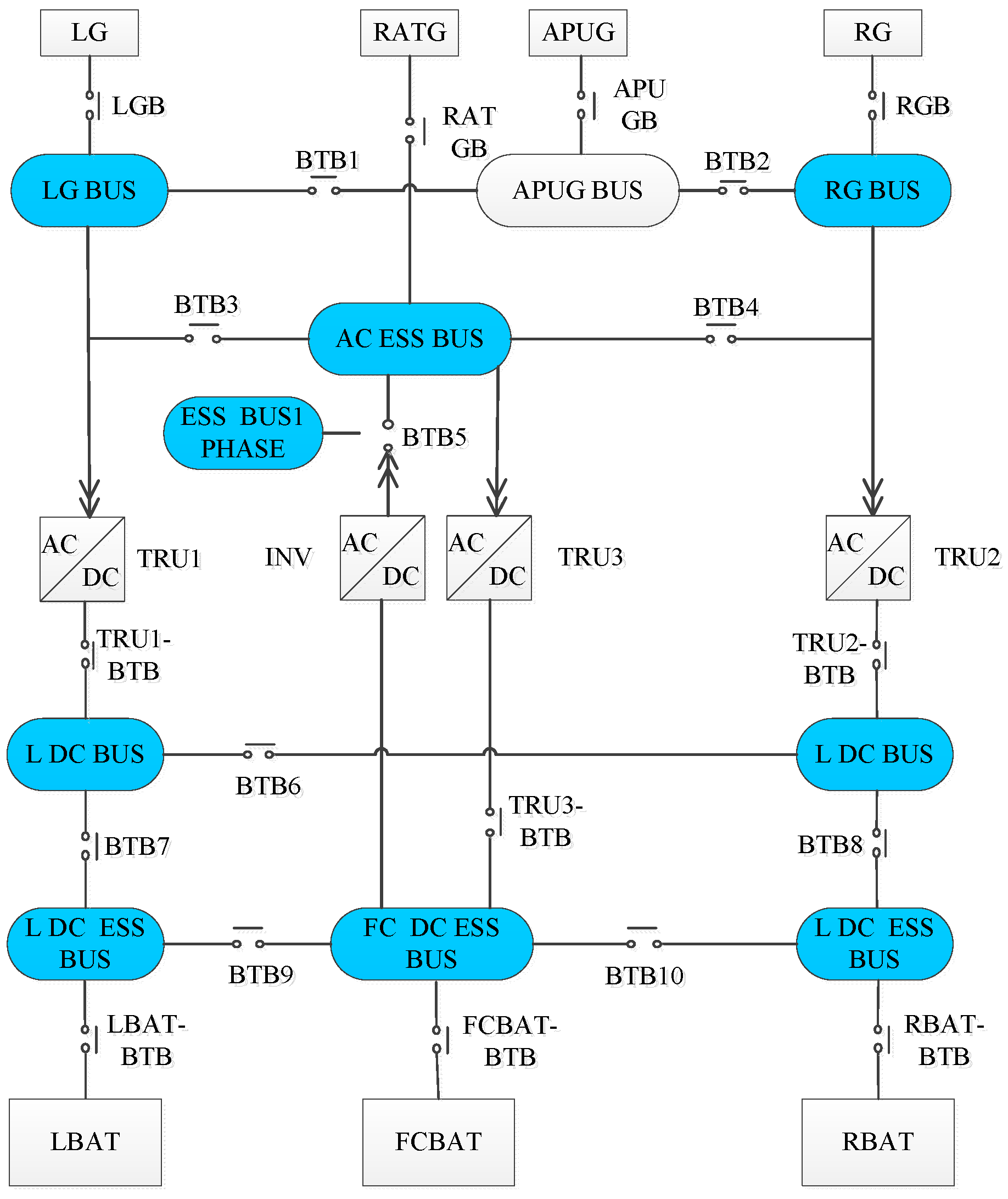
2.1. The Architecture of AEPS in the Design Stage

An AEPS was designed to provide electrical energy for the entire aircraft’s electrical load including avionics equipment, de-icing systems, navigation systems, flight control systems, etc. How to select suitable components to build a power distribution network/architecture that meets the power requirements of the entire aircraft is the primary task in the design stage of AEPS [38]. A typical AEPS is shown in Figure 1 and see [39,40,41] for more similar AEPS.
In Figure 1, four generators are included: one left and one right alternating current variable frequency generators indicated as LG and RG separately, an auxiliary power unit generator (APUG), and an emergency power unit-ram air turbine generator (RATG). The generators RG and LG work independently and are the backup for each other; when both of them fail, APUG and RATG serve as backups to provide electrical power for the safety-critical equipment. In addition, there are some batteries (e.g., left and right batteries (LBAT, RBAT)) and flight control batteries (FCBAT). In particular, components such as generators and batteries that serve as an electrical power source in the AEPS architecture are defined as source nodes, and the busbars/buses that directly support the operation of selected electrical loads are defined as sink nodes, from which the required power of the loads (e.g., navigation system, flight control system, etc.), is obtained.
It can be seen that an AEPS in the design stage is essentially a directed topology network with a “source–network–sink” structure including four basic functions: power generation, power storage, power distribution, and load support [16]. Moreover, “source” is the starting point of the network used to perform power generation and storage function; “sink” is the end point of the network used to perform the load support function; “network” includes all the components between sources and sinks (e.g., contactors, inverters, etc.) used to perform the function of distribution.

2.2. AEPS Reliability Design

System reliability design refers to taking reliability into consideration in the system design stage, which requires designers not only to consider that the designed system can provide sufficient electrical power to complete the power supply function, but also to evaluate the power supply reliability of the designed system [42,43]. When the evaluation results are unsatisfactory, the design needs to be revised: re-build the structure of the network or re-select better performance components until the reliability requirements are met (see Figure 2).
As shown in Figure 2, the core of system reliability design lies in two points: (1) how to compute the reliability of the designed system; and (2) how to modify the system that does not meet the reliability requirements.
For point (1), unlike the general system having one probability to quantify its reliability, since the function of AEPS is to distribute power from source nodes to sink nodes, the reliability computation of AEPS is to calculate the probability of each sink node that obtains electrical power successfully from source nodes under stated conditions for a given system time T. That is to say, the system-level reliability of AEPS means the power supply reliability of each sink node. For example, the AEPS in Figure 1 contains sink nodes (e.g., left AC power supply busbar (LG BUS), right AC power supply busbar (RG BUS), essential three-phase alternating current busbar (AC ESS BUS), essential single-phase alternating current bus (ESS BUS 1 PHASE), etc.), so the system reliability of the AEPS refers to the power supply reliability of these sink nodes under system time T. Moreover, on the basis of Figure 2, the method for computing the power supply reliability of the designed AEPS is illustrated as follows.
Assume that an AEPS is composed of n components with failure rates λ = [ λ 1 , λ 2 , λ n ], of which Num sink nodes are included. Failure rate λ ( t ) refers to the probability of the component that has not failed at time point t to fail in the next per unit time. The failure rate λ(t) of a component is often described by the Bath–Tub curve. It has three periods: early failure period, accidental failure period, and wear out period. In AEPS, components usually operate during the accidental failure period (so this period is also called using life), where λ(t) can be roughly regarded as a constant value λ if the operation environment is steady and unchanged. Therefore, the failure probability of the i-th component can be expressed as if we do not consider the operation environment changes:
P i = 1 e λ i T
Furthermore, in theory, in combination with the failure/function logical relationship between the failure of components and power loss of sink nodes, formula R s y s , s = F ( λ , T ) can be obtained and computed, 1 ≤ sNum. R s y s , s represents the power supply reliability of the sink nodes s, and F ( λ , T ) represents the power supply reliability function with the component failures rate as variables. When each component failure rate is constant, power supply reliability is a function of time T, as shown in Figure 3. In addition, since system reliability model can effectively express the logics between the failures of the component-level and system-level, the formula R s = F ( λ , T ) can be obtained with the help of the system reliability model. The commonly used system reliability model of AEPS includes minimal path sets, minimal cut sets, fault tree, and reliability block diagram. Equation (2) is the formula for calculating the power supply reliability of the s-th power supply sink node by using the minimal path sets [32].
R s = P ( i = 1 m A i ) = i = 1 m P ( A i ) i < j m P ( A i A j ) + i < j < k m P ( A i A j A k ) + + ( 1 ) m 1 P ( i = 1 m A i )
In Equation (2), m is the number of the minimal path sets of sink nodes s, and A i represents the i-th minimal path set. A minimal path set refers to a set of components to ensure the normal operation of the system; any component failure in the set will cause the path set failure, and the system fails when, and only when, all the path sets fail. For the method of obtaining the minimal path sets of each sink node, please refer to [17].
According to Equations (1) and (2) and Figure 3, it can be seen that if all the component failure rates are constant, the reliability of each power supply sink node obtained is also constant under the system time T. However, as mentioned in Section 1, subject to epistemic uncertainty and changing flight environments, it is more appropriate to regard component failure rate as a random variable. At this time, as the dependent variable of the component failure rate, at a given system time T, R s should be a non-deterministic value represented by a probability distribution, which can help the designers to fully understand the uncertainty degree of the reliability of the designed system. However, uncertainty means risk. If the uncertainty of reliability is high, how to reduce uncertainty to ensure the stability of flight reliability is a more relevant issue for the designer. As shown in Figure 2, system reliability design is an iterative process, and there is no doubt that developing a satisfactory system only just through expert experience is time expensive. If there are scientific methods to guide designers to reduce system reliability uncertainty, the system design cycle will definitely be greatly reduced. However, thus far, there is no relevant research, which is the main motivation of this research.

3. Importance Measure Index and Calculation Method

The failure uncertainty of component level will propagate to the failure uncertainty of system level, leading to the uncertainty risks of the system during operation. To reduce system-level uncertainty effectively in the design stage, this section proposes an importance measure index to measure the contribution of the uncertainty of the component failure rate to the uncertainty of the power supply reliability as well as an algorithm for computing the index presented on the basis of the AEPS reliability calculation method described in Section 2. The ranking of the obtained index can quickly lock the key components with high contribution to system-level reliability uncertainty and provide theoretical guidance for designers to revise the system design: priority to improve the performance of the key components can more effectively reduce the uncertainty of system reliability.

3.1. Importance Measure Index

In order to reasonably measure the influence of the uncertainty of the failure rate λ of each component on the power supply reliability of the sink nodes s given a system time T, the importance measure index η s , i 2 in Equation (3) can be defined according to the variance decomposition theory [44,45].
η s , i 2 = V a r s , λ i [ E s , λ i ( R s | λ i ) ] V a r s [ R s ]
In Equation (3), the subscript s represents the s-th sink node of AEPS, s = 1, 2, …, Num; the subscript i represents the i-th component in the system, i = 1, 2, …, n; ~i represents the rest components of the system except for component i; λ ~ i represents the vector of the failure rates of the remaining components of the system except for λ i , for example, for a system containing four components, if i = 2, then λ ~ i = { λ 1 , λ 3 , λ 4 } ; η s , i 2 is the proposed importance measure index to measuring the uncertainty contribution of the i-th component failure rate on the uncertainty of the supply reliability of the sink node s. V a r s [ R s ] is the unconditional variance of power supply reliability of the sink node s; E s , λ ~ i ( R s | λ i ) is the conditional expected value of power supply reliability of the sink node s, and to be specific, it is on the condition that the failure rate of the i-th component is given; accordingly, V a r s , λ i [ E s , λ ~ i ( R s | λ i ) ] is the variance of E s , λ ~ i ( R s | λ i ) .

3.2. Calculation Method

Based on the Monte Carlo simulation theory [20,32], this paper proposed a method to estimating η s , i 2 (i = 1, 2, …, n, s = 1, 2, …, Num), which includes six steps. The pseudocode of the algorithm is shown in Algorithm 1, and the steps are explained below.
Step 1: Establish a failure rate sample vector λ i = [ λ i 1 ,   λ i 2 ,   ,   λ i M ] for component i.
According to the probability distribution function F( λ i ) that variable λ i obeys, the inverse transformation method is adopted to generate M samples to form the sample vector λ i = [ λ i 1 ,   λ i 2 ,   ,   λ i M ] . Specifically, generate M random variables U1, U2, …, UM from the uniform distribution in the interval [0, 1] first, which is U~Uniform(0, 1). Then, use the inverse distribution function F1(U) to calculate the random variable λ i j : λ i j = F 1 ( U j ) , j = 1, 2, …, M.
Step 2: Establish a component failure rate sample matrix λ ~ i | λ i .
Similarly, for λ i j (j = 1, 2, …, M) in vector λ i , use the inverse transformation method to generate sample λ ~ i j , k (k = 1, 2, …, C) from the conditional probability distribution f λ ~ i ( λ ~ i | λ i j ) to form the component failure rate sample matrix λ ~ i | λ i (j = 1, 2, …, M), see Equation (4).
λ ~ i | λ i = λ i 1 λ i 2 λ i M [ λ ~ i 1 , 1 λ ~ i 1 , 2 λ ~ i 1 , C λ ~ i 2 , 1 λ ~ i 2 , 2 λ ~ i 2 , C λ ~ i M , 1 λ ~ i M , 2 λ ~ i M , C ]
In the reliability analysis of AEPS, the failures between different components are generally considered to be independent of each other, so formula f λ ~ i ( λ ~ i | λ i j ) = f λ ~ i ( λ ~ i ) is established. In the component failure rate sample matrix λ ~ i | λ i , the element λ ~ i j , k is the k-th vector composed of the failure rates of the remaining components of the system under the failure rate λ i j . For example, for the power supply bus s, if there are four components that affect its power supply reliability in the system, then for the 2nd component (i = 2), the vector in the proposed matrix is donated as λ ~ i j , k = [ λ 1 j , k , λ 3 j , k , λ 4 j , k ] .
Step 3: Calculate the power supply reliability matrix Rs of the sink nodes s.
Substitute the sample point [ λ i j , λ ~ i j , k ] of the obtained component failure rate sample matrix into Equation (2) to calculate the power supply reliability R s j , k = F s ( λ i j , λ ~ i j , k ) of the sink nodes s, of which F s represents the function with the state of each component in the system as a variable and the power supply state of the sink nodes s is a dependent variable. It is clear that R s j , k (j = 1, 2, …, M, k = 1, 2, …, C) can form an output matrix Rs with size M × C;
Algorithm 1: Importance_Calculation (Lanbuda[][], Distribution_type[], s, Path_set[][], T, RELI_var[])
//Input: array Lanbuda with size S × N, Distribution_type with size N, Path_sets with size Num × N, variable s and T. N is the component number in the MPSs of sink node s. S is the max number of parameters that used to describe the probability distribution of each component’s failure rate, e.g., there are two components in the MPSs of sink node s, and the failure rates of the first and the second component follow lognormal and triangular distributions, respectively, which are described with two and three parameters in separate, so S = 3. The ith element represents the distribution type of component i’s failure rate, and the ith column of Lanbuda stores the probability distribution parameters of node i’s failure rate. Num represents the number of MPSs of sink node s and the ith row of Path_sets stores the components in the ith MPS. T represents system time.
//Output: array RELI_var with size N. Its ith element represents component i’s importance degree that measures the contribution to the uncertainty of node s’s power supply reliability.
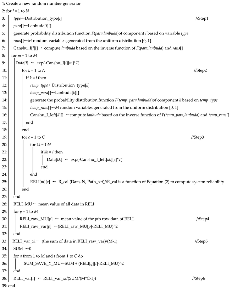
Applsci 12 02857 i001
Step 4: Estimate the value of E s , λ ~ i ( R s | λ i j ) .
For j-th row of the output matrix Rs, j = 1, 2, …, M, use Equation (5) to calculate the mean reliability.
R ^ s ( λ i j ) = 1 C k = 1 C R s j , k E s , λ ~ i [ R s | λ i j ]
The term E s , λ ~ i ( R s | λ i j ) indicates the expected value of the power supply reliability of the sink nodes s when the failure rate of the component i takes the value λ i j .
Step 5: Estimate the unconditional variance of power supply reliability and the variance of E s , λ ~ i ( R s | λ i j ) .
For the power supply reliability of sink nodes s, estimate its value of expectation using Equation (6). Then, with the help of Equation (7), calculate the estimation value V ^ a r s , λ i [ E s , λ ~ i ( R s | λ i ) ] of variance V a r s , λ i [ E s , λ ~ i ( R s | λ i ) ] . Finally, use Equation (8) to calculate the estimation value V ^ a r s [ R s ] of variance V a r s [ R s ] :
R ¯ s = 1 M j = 1 M R ^ s ( λ i j ) E s [ R s ]
V ^ ar s , λ i [ E s , λ ~ i ( R s | λ i ) ] = 1 M - 1 j = 1 M [ R ^ s ( λ i j ) R ¯ s ] 2
V ^ a r s [ R s ] = 1 M C - 1 j = 1 M k = 1 C ( R s j , k R ¯ s ) 2
Step 6: Compute the estimation value of the proposed importance measure index η ^ s , i 2 .
Substitute the results of Equations (7) and (8) into Equation (9), the importance measure index of component I, which can quantify its failure uncertainty contribution to the power supply reliability uncertainty of the sink node s, is estimated.
η ^ s , i 2 = V ^ a r s , λ i [ E s , λ ~ i ( R s | λ i ) ] V ^ a r s [ R s ]
The physical meaning of the six steps is explained as follows. First, each element in j-th row of the matrix λ ~ i | λ i stands for the failure rate sample of the remaining components when the i-th component takes the value λ i j . Accordingly, for the power supply reliability matrix Rs obtained through the matrix λ ~ i | λ i , each element in its j-th row represents a possible value of the power supply reliability of sink node s when the failure rate of component i takes the value λ i j , and the mean value of the j-th row is R ^ s ( λ i j ) by averaging C possible values of the row. In addition, according to the law of large numbers, as the value of C increases, R ^ s ( λ i j ) will surely converge to the expectation E s , λ ~ i ( R s | λ i j ) ; moreover, when the two samples λ i j and λ i j + 1 of the failure rate of the i-th component are the same, the mean value R ^ s ( λ i j ) and R ^ s ( λ i j + 1 ) tend to be the same as C increases. That is to say, for the row mean value R ^ s ( λ i 1 ) , R ^ s ( λ i 2 ) ,   ,   R ^ s ( λ i M ) of the matrix Rs, the numerical difference between them is mainly caused by the different failure rate values of component i. Therefore, the variance V ^ a r s , λ i [ E s , λ ~ i ( R s | λ i ) ] , calculated by Equation (7), quantifies the degree of dispersion of the power supply reliability of the sink nodes s induced by the dispersion of the failure rate of the component i. Since the uncertainty of output propagated from input can be measured with the variance of the output variable [44], the variance computed by Equation (7) has the ability to quantify the uncertainty of the failure rate of component i on the contribution of the power supply reliability uncertainty of the sink node s. Furthermore, because the variance calculated by Equation (8) is based on all the elements in the matrix Rs and the matrix includes all the possible values of the power supply reliability of the sink node s, the obtained variance V ^ a r s [ R s ] is a measurement that quantifies the failure uncertainty contribution of all the components to the uncertainty of the power supply reliability of the sink node s.
In summary, first, the ratio of variance V ^ a r s , λ i [ E s , λ ~ i ( R s | λ i ) ] to variance V ^ a r s [ R s ] calculated by Equation (9) essentially quantifies the ratio of the uncertainty that the i-th component contributes to and the whole uncertainty that all the components contribute to in theory; and according to the law of large numbers, with S , C , i = 1 n η ^ s , i 2 1 holds. This means that if the simulation results obtained by the proposed method satisfies the convergence condition: i = 1 n η ^ s , i 2   1 , it indicates that the sampling sizes M and C are reasonable, otherwise, the sampling size needs to be increased until the convergence condition is met. Second, from the index definition of Equation (3) and the above explanation, it can be seen that this index value varies in the range [0, 1]. Furthermore, the higher the index value of one component, the greater the influence of the uncertainty of the component’s failure rate on the uncertainty of system reliability, and vice versa. Therefore, the index can help designers identify which components are more important to the system to reduce the system reliability uncertainty, and the quality and performance of these components with a higher index can be prioritized to be improved. Conversely, improving components with lower index will not achieve better results. Algorithm 1 shows the pseudocode of the proposed algorithm for computing the importance degree.

4. Case Studies

AEPS is essentially a complex network system, which is a composite form of series and parallel. Therefore, a typical series-parallel system was taken as an example to demonstrate the correctness of the proposed index and algorithm. The method was also applied to an AEPS of the real world to further verify the rationality, and then the significance of the proposed index for system reliability uncertainty risk reduction in the system reliability design was analyzed. Finally, based on the index, the “number and degree optimization criterion” for guiding designers to improve the system reliability is put forward and discussed.

4.1. Uncertainty Analysis of Series-Parallel Systems

4.1.1. Case Description

Figure 4 shows a series-parallel system consisting of four components C1, C2, C3, and C4. Four cases with different failure uncertainty levels of components are given:
Case   1 :   C 1 :   μ λ 1 = 3.5066 ,   δ λ 1 = 0 ;   C 2 :   μ λ 2 = 3.5066 ,   δ λ 2 = 0 ;   C 3 :   μ λ 3 = 3.5066 ,   δ λ 3 = 0 ;   C 4 :   μ λ 4 = 3.5066 ,   δ λ 4 = 0 ; Case   2 :   C 1 :   μ λ 1 = 3.5066 ,   δ λ 1 = 0.05 ;   C 2 :   μ λ 2 = 3.5066 ,   δ λ 2 = 0.05 ;   C 3 :   μ λ 3 = 3.5066 ,   δ λ 3 = 0.05 ;   C 4 :   μ λ 4 = 3.5066 ,   δ λ 4 = 0.05 ; Case   3 :   C 1 :   μ λ 1 = 3.5066 ,   δ λ 1 = 0.05 ;   C 2 :   μ λ 2 = 3.5066 ,   δ λ 2 = 0.1 ;   C 3 :   μ λ 3 = 3.5066 ,   δ λ 3 = 0.05 ;   C 4 :   μ λ 4 = 3.5066 ,   δ λ 4 = 0.1 ; Case   4 :   C 1 :   μ λ 1 = 3.5066 ,   δ λ 1 = 0.05 ;   C 2 :   μ λ 2 = 3.5066 ,   δ λ 2 = 0.025 ;   C 3 :   μ λ 3 = 3.5066 ,   δ λ 3 = 0.05 ;   C 4 :   μ λ 4 = 3.5066 ,   δ λ 4 = 0.025 .
In these four cases, the failure rate of each component obeys a lognormal distribution, expressed with two parameters of the mean μ λ i and standard deviation δ λ i . To discuss the impact of component failure rate uncertainty on system reliability, the mean values of four cases were set to be the same value and the standard deviation was set to different values in the four cases. In particular, δ λ i = 0 was set in case 1, which means that the failure rate of each component was a constant value and no uncertainty of reliability was considered in this case.

4.1.2. Calculation and Analysis

As a seven-hour flight is general in the real world, system time T = 7 h was set here to verify the proposed method, and then the stated Monte Carlo simulation method was applied to the four cases, with the results shown in Figure 5 and Table 1. The Monte Carlo simulation method includes three steps: first, given the system time t0, according to the probability density function of the component failure rate λ, generate N group samples λk = (λk1, λk2, …, λkn), (k = 1, …, N), and substitute λk and t0 into Equation (1) to obtain the vector pk = (pk1, pk2, …, pkn); second, substitute pk into Equation (2) to compute the sink node’s power supply reliability Rk, forming a reliability vector R(t0) = (R1, R2, …, RN); finally, sort the elements in vector R(t0) from small to large, and calculate its confidence interval under the given confidence interval as well as plot the kernel density function curve. Furthermore, the proposed algorithm for computing the importance degree index of each component based on the variance decomposition was performed on the four cases separately, and the results are shown in Table 2. The results of the four cases are discussed below.
(1) From Table 2, it can be seen that all of the components’ importance measure indicators equaled to zero in case 1. That is because the failure rate of each component in the system was constant and had no effect on the uncertainty of system reliability. It is clear that this result is consistent with engineering practice.
(2) In case 2, the importance measure indicators of components C3 and C4 were equal, and the importance measure indicators of components C1 and C2 were equal. The result correctly reflects the fact that components C1 and C2 took the same structural position and had the same failure parameters in the system, and similarly, components C3 and C4 took the same structural position and had the same failure parameters in the system. In addition, since components C1 and C2 formed a parallel structure, the system will only fail when both of them fail, while components C3 and C4 were in a series structure, and the system will fail when either of them fails. That is to say, C3 and C4 are more important than C1and C2, so under the condition that the failure rate parameters of all the four components are identical, the components C3 and C4 definitely will cause a greater impact on the system reliability uncertainty than components C1 and C2, which is consistent with the results of Table 2.
(3) In case 3, component C4 had the highest degree of uncertainty in failure rate and its structural position was more important than components C1 and C2, so the value of its importance measure indicator must be the maximum; in contrast, the failure rate uncertainty of component C1 was the lowest and its structural position was less important than components C3 and C4, so the value of its importance measure indicator must be the minimum. The analysis is consistent with the importance measure indicators ranking: C4, C3, C2, and C1, obtained through the proposed method.
(4) In case 4, component C3 had the largest variance in failure rate and took the most important structural position in the system, so the importance measure indicator was the highest; components C1 and C2 were structurally equivalent while C1 had higher uncertainty in failure rate than C2, so the importance measure indicator of component C1 was necessarily higher than C2; components C2 and C4 had the same failure rate parameters while C4 was structurally more important than C2, so the importance measure indicator of component C4 was necessarily higher than C2; in a word, the importance measure indicators ranking must be: C3, C4, C1 and C2, the same as the results in Table 2.
In summary, the above analysis shows that the proposed importance measure index with its calculation method can correctly calculate and measure the degree of influence of component failure uncertainty on system reliability uncertainty.

4.2. Reliability Uncertainty Analysis on an AEPS

4.2.1. Case Description

The AC subsystem of the AEPS shown in Figure 1 was taken as an example to illustrate the proposed method. The AC subsystem supply power to the AC electrical equipment mainly through two sink nodes: LG BUS and RG BUS. The sink node LG BUS has three minimal path sets: {LG BUS,LGB,LG}, {APUG,APUGB,APUG BUS,BTB1,LG BUS}, and {RG,RGB,RG BUS,BTB2, APUG BUS,BTB1,LG BUS}; the sink node RG BUS also has three minimal path sets: {RG, RGB,RG BUS}, {APUG,APUGB,APUG BUS,BTB2,RG BUS}, and {LG,LGB,LG BUS, BTB1,APUG BUS,BTB2,RG BUS}. Eleven components are involved in these six minimal path sets, which are LG, LGB, LG BUS, BTB1, APUG BUS, APU GB, APUG, BTB2, RG BUS, RGB, and RG. For the convenience of description, the components are numbered from 1 to 11. The failure rate of each component obeys a triangular distribution and the parameters are shown in Table 3. In aircraft engineering, by taking the general changes of flight conditions into consideration, different experts may have different opinions on the exact value that the component’s failure rate should be, but they always have a consensus on the order of magnitude of the failure rate. In addition, triangle distribution is always widely used in depicting a random variable that one only knows its maximum, minimum, and the most likely value. Therefore, we used the component’s failure rate as a variable that obeys the triangle distribution, where the mode parameter λmode is the value that is repeated most often in [14,17], and the upper limit parameter λupper and lower limit parameter λlower is the maximum and minimum value in the magnitude order of λmode. Since RG BUS and LG BUS are completely symmetrical in structure, the power supply reliability of them is equal, and the contribution of component failure uncertainty to the power supply reliability uncertainty of the sink node LG BUS is discussed here.

4.2.2. Calculation and Analysis

Aircraft are routinely inspected systematically every 1000 h, so T = 1000 was set here. The results of the importance measure indicators of these eleven components computed through the proposed algorithm are presented in Table 4. From the perspective of the rationality and the engineering application value, the results are discussed.
(1) In order to verify the correctness of the proposed method and the significance of the proposed importance measure index to the improvement of system reliability in the design stage, the system was optimized according to the results in Table 4.
Table 4 shows that components LG BUS and BTB1 contributed most to the uncertainty of power supply reliability of the sink node LG BUS, followed by components LGB and LG. The importance measure indicator values of these four components were 0.3803, 0.3636, 0.1306, and 0.097, respectively, and the total value of the four indicators was 0.97, which means that the contribution of the four components to the power supply reliability uncertainty of the sink node s had the ratio of 0.97. In contrast, the other seven components only contributed 0.023 to the uncertainty of power supply reliability. Therefore, in order to reduce the power supply reliability uncertainty, reducing the failure uncertainty of LG BUS and BTB1 should be the first solution to optimize the system, and if the reliability uncertainty of the optimized system is still high, reducing the failure uncertainty of these four components LG BUS, BTB1, LGB, and LG can also be a good solution. In Table 5, five system reliability improvement/optimization solutions are put forward.
As a system reliability optimization measure, reselecting components of less fluctuation in failure rate with flight environment changes means replacing the previous original components with new but the same functional components of more stable performance, which inevitably increases the procurement cost. For the convenience of the analysis, it was assumed that the failure rate of the new, more stable reselected component in each solution did not vary with the flight environment and was a constant value that equaled λmode in Table 3, while the failure rates of the remaining components still followed the previous triangular distribution. In fact, it is impossible for the component failure rate to remain unchanged with the flight environment, which is an extreme assumption made here to more significantly demonstrate the validity of the proposed method in this paper.
The Monte Carlo simulation method was used to compute the power supply reliability of the sink node LG BUS under the five system reliability improvement solutions, and the results are shown in Table 6 and Figure 6. In Table 6, “Importance degree” refers to the proposed importance measure index of each component, which quantifies the contribution of the uncertainty of each component’s failure rate to the uncertainty of the reliability of the LG BUS power supply, calculated by the method in Section 3.2; “Mean value”, “Variance”, and “Confidence” in Table 6 represent the mean, variance, and 95% confidence interval of the reliability of the original system and the five optimized systems, respectively; “Reduction degree” refers to the degree by which the uncertainty of system reliability is reduced after the system is optimized and because the variance can be used to characterize the degree of the system reliability uncertainty, the reduction degree can be calculated by the formula: reduction degree = 1.0-variance of the optimized system/variance of the original system; “Improved effect ranking” represents the improvement effect of the five solutions, which is obtained based on the data of reduction degree; and finally, “Original” represents the original system without any optimization measure, so the “original” row does not involve the data of “Importance degree”, “Reduction degree”, and “Improved effect ranking”. The improvement results in Table 6 and Figure 6 are discussed from two points.
First, in terms of improvement effect, all five solutions could reduce the degree of system reliability uncertainty, and it can be seen that the data in the “Reduction degree” column is consistent with the data in the “Importance degree” column. That is, the system reliability improvement effect is consistent with the importance measure index of each component, which shows that the proposed importance measure index can indeed reflect the uncertainty contribution of each component’s failure rate to the system reliability uncertainty.
Second, the results showed that the more components improved did not necessarily lead to a better system reliability improvement effect. This means that if there is no guidance of the importance measure index in system reliability design practice, the designers could have improved many components, but it is still difficult to achieve a good improvement effect, resulting in a longer design cycle. For example, compared to the other four solutions, solution 5, which improved the most components, had the poorest effect in system reliability improvement. That is, because in solution 5, though seven components were improved, the sum of the importance measure indicators of these components was only 0.23. In contrast, the importance measure index of both the component LG BUS and BTB was greater than 0.35, which definitely led to the improvement of solution 1 and 2 being better than solution 5, though only one component was improved in the former two solutions.
To be more specific, if the designers want to improve the system with only one component, there are 11 solutions; if the designers want to improve the system with two components, there are C 11 2 = 55 solutions; if the designers want to improve the system with three components, there are C 11 3 = 165 solutions, and so on. In the face of such a huge number of optional solutions, if there is no importance measure index providing guidance, the formulation of improvement solutions in the system reliability design stage will inevitably become blind, and difficult to work. Obviously, as the number of components in the system increases, the problem becomes more difficult. In contrast, since the proposed importance measure index can correctly reflect the contribution of components to the uncertainty of system reliability, then according to the components’ ranking of the index from high to low, the effect of components on the improvement in system reliability will decrease in turn. Based on this, the designer can quickly propose an effective optimization solution from the huge number of options.
(2) Based on the ranking of the proposed importance measure indicators from high to low and the analysis in point (1), this paper summarizes the “quantity and degree optimization criteria” for system reliability design.
The criterion is described as follows. (i) When the number of components that can be optimized/reselected is required to be m at most, the sum value w% (ƞ1 + ƞ2 + … + ƞm = w%) of the importance measure indicators of the first m components in the index ranking determines that the degree by which the system reliability uncertainty can be reduced. (ii) When the degree of system reliability uncertainty is required to be reduced by w% at least, and if the sum of the importance measure indicators of the first m components in the ranking satisfies the inequality ƞ1 + ƞ2 + … + ƞmw% and ƞ1 + ƞ2+ … + ƞm−1w%, then to meet the requirement above, at least m components are required to be optimized/reselected.
This criterion is illustrated with the results obtained in this system. For criterion (i), if a maximum of three components are required to optimize the system, and the top three components in the index ranking are LG BUS, BTB1, and LGB, the sum value 0.8745 of the importance indicators of the three components determines that the uncertainty of system reliability can be reduced by 87.45% at most. For criterion (ii), if the uncertainty degree of system reliability is required to be reduced by at least 90%, as the importance index sum value of the first three components is 0.8745 and the importance index sum value of the first four components is 0.9715, four components at least should be improved to meet the design requirements.
This criterion clarifies the corresponding relationship between the number of components to be improved and the degree of system reliability improvement, which helps designers quickly formulate a solution that meets the design reliability requirements; in addition, it can also help decision makers put forward reasonable system reliability improvement requirements to ensure that the proposed system reliability design task is theoretically feasible. For instance, when the importance measure index of component LG BUS is 0.3793, then the uncertainty of system reliability cannot be reduced by 50% only by improving the performance of this component; furthermore, to achieve the goal of 50%, at least component BTB1 should also be improved. Correspondingly, if the design requirement is to reduce the uncertainty of the system reliability to 50% only by improving one component, then the design requirement cannot be achieved theoretically, which should not be put forward.
In summary, the above analysis not only verifies the correctness of the proposed index and calculation method, but also indicates the significance of the proposed index and the “quantity and degree optimization criterion” for improving system reliability in the design stage.

5. Conclusions

As the uncertain risk of an electrical power system has become a great concern for safe flight, this paper studied the problem of how to reduce the uncertainty of the power supply reliability by reducing the component failure rate uncertainty in the aircraft electrical power system reliability design stage. Two points can be summarized.
First, an importance measure index was proposed based on variance decomposition theory, and then the calculation method with its corresponding algorithm was presented. In addition, not only was the rationality of the proposed index explained in theory, but the proposed method was also applied to a general series-parallel system and a real-world aircraft electrical power system. The results showed that the proposed index with its calculation algorithm could correctly measure and calculate the contribution of the component failure rate uncertainty to the power supply reliability uncertainty.
Second, based on the proposed importance measure index, a criterion named as “quantity and degree optimization criteria” to reduce the system reliability uncertainty was put forward in the system reliability design stage. This criterion specifies the correspondence between the number of components to be improved and the degree of system reliability improvement to efficiently help designers develop a solution that meets the requirements for system reliability design and help decision makers propose reasonable improvement requirements, ensuring the proposed task’s theoretical feasibility.
In summary, the proposed method including an importance measure index and a calculation method in this paper can effectively assist designers to quickly reduce the uncertainty of power supply reliability, thus reducing the system development cycle in the system design stage, reducing the uncertain risks and ensuring flight safety in the subsequent operation stage. Theoretically speaking, priority to reduce the uncertainty of components with higher importance indicators can better improve the stability of the system reliability, but the corresponding economic cost of the components to be improved may be higher or difficult to implement in technology. Therefore, the follow-up research will also take the constraints of economic and technical feasibility into the considerations of system reliability optimization.

Author Contributions

Conceptualization, Y.W. and X.H.; methodology, Y.W.; software, Y.C.; validation, Y.W. and Y.C.; formal analysis, X.H.; investigation, X.H.; resources, X.G.; data curation, S.L.; writing—original draft preparation, Y.W.; writing—review and editing, Y.C.; visualization, X.G.; supervision, Y.L.; project administration, S.L.; funding acquisition, Y.W. and Y.L. All authors have read and agreed to the published version of the manuscript.

Funding

The research was funded by the Natural Science Foundation of Shaanxi Province under Award 2021JQ-490.

Acknowledgments

The authors thankfully acknowledge the support provided by the Natural Science Foundation of Shaanxi Province. The first author also would like to thank Fengtao Wang, whose valuable comments helped the quality of this work improve significantly.

Conflicts of Interest

The authors declare no conflict of interest.

References

  1. Buticchi, G.; Costa, L.; Liserre, M. Improving system efficiency for the more electric aircraft: A look at dc\/dc converters for the avionic onboard dc microgrid. IEEE Ind. Electron. Mag. 2017, 11, 26–36. [Google Scholar] [CrossRef]
  2. Barzkar, A.; Ghassemi, M. Electric power systems in more and all electric aircraft: A review. IEEE Access 2020, 8, 169314–169332. [Google Scholar] [CrossRef]
  3. Pandian, G.; Pecht, M.; Enrico, Z.I.O.; Hodkiewicz, M. Data-driven reliability analysis of Boeing 787 Dreamliner. Chin. J. Aeronaut. 2020, 33, 1969–1979. [Google Scholar] [CrossRef]
  4. Denning, S. What went wrong at Boeing. Strategy Leadersh. 2013, 41, 36–41. [Google Scholar] [CrossRef] [Green Version]
  5. Boeing 787 Makes Emergency Landing in Japan over Battery. 2013. Available online: https://www.cbsnews.com/news/boeing-787-makes-emergency-landing-in-japan-over-battery/ (accessed on 21 November 2021).
  6. Boeing 787 Probe Far from Complete. 2013. Available online: https://www.chinadaily.com.cn/world/2013-01/25/content_16173038.htm (accessed on 21 November 2021).
  7. Wang, W. Chinese Authorities Keep Close Tabs on Dreamliner Woes. 2013. Available online: http://www.chinadaily.com.cn/business/2013-01/18/content_16138334.htm (accessed on 21 November 2021).
  8. Keshavarzi, E.; McIntire, M.; Goebel, K.; Tumer, I.Y.; Hoyle, C. Resilient system design using cost-risk analysis with functional models. In Proceedings of the International Design Engineering Technical Conferences and Computers and Information in Engineering Conference. American Society of Mechanical Engineers (ASME), Cleveland, OH, USA, 6–9 August 2017. [Google Scholar]
  9. Menu, J.; Nicolai, M.; Zeller, M. Designing Fail-Safe Architectures for Aircraft Electrical Power Systems. In Proceedings of the 2018 AIAA/IEEE Electric Aircraft Technologies Symposium (EATS), Cincinnati, OH, USA, 12–14 July 2018. [Google Scholar]
  10. Alves, G.; Marques, D.; Silva, I.; Guedes, L.A.; da Silva, M.D.G. A methodology for dependability evaluation of smart grids. Energies 2019, 12, 1817. [Google Scholar] [CrossRef] [Green Version]
  11. Cai, L.; Zhang, L.; Yang, S.; Wang, L. Reliability assessment and analysis of large aircraft power distribution systems. Acta Aeronaut. Astronaut. Sin. 2011, 32, 1488–1496. [Google Scholar]
  12. Kritzinger, D. Aircraft System Safety: Military and Civil Aeronautical Application; Woodhead Publishing: Cambridge, UK, 2006. [Google Scholar]
  13. Telford, R.D.; Galloway, S.J.; Burt, G.M. Evaluating the reliability & availability of more-electric aircraft power systems. In Proceedings of the 2012 47th International Universities Power Engineering Conference (UPEC), Uxbridge, UK, 4–7 September 2012. [Google Scholar]
  14. Zhao, Y.; Che, Y.; Lin, T.; Wang, C.; Liu, J.; Xu, J.; Zhou, J. Minimal cut sets-based reliability evaluation of the more electric aircraft power system. Math. Probl. Eng. 2018, 2018, 9461823. [Google Scholar] [CrossRef] [Green Version]
  15. Zhao, Y.; Wu, H.; Cai, J.; Shi, X. Reliability analysis for electric power systems of more-electric aircraft based on the minimal path set. J. Comput. Methods Sci. Eng. 2019, 19, 1017–1026. [Google Scholar] [CrossRef]
  16. Zhang, Y.; Kurtoglu, T.; Tumer, I.Y.; O’Halloran, B. System-Level Reliability Analysis for Conceptual Design of Electrical Power Systems. In Proceedings of the Conference on Systems Engineering Research (CSER), Redondo Beach, CA, USA, 15–16 April 2011. [Google Scholar]
  17. Wang, Y.; Yang, M.; Miao, Z.; Dong, X. A Reliability Modelling Method for Aircraft Electrical Power System Based on Probability Network. In Proceedings of the 2018 5th International Conference on Mathematics and Computers in Sciences and Industry (MCSI), Corfu, Greece, 25–27 August 2018. [Google Scholar]
  18. Kong, X.; Wang, J.; Zhang, Z. Reliability analysis of aircraft power system based on Bayesian network and common cause failure. Acta Aeronaut. Astronaut. Sin. 2020, 41, 70–279. [Google Scholar]
  19. Han, L.; Wang, Y.B.; Zhang, Y.; Lu, C.; Fei, C.W.; Zhao, Y.J. Competitive cracking behavior and microscopic mechanism of Ni-based superalloy blade respecting accelerated CCF failure. Int. J. Fatigue 2021, 150, 106306. [Google Scholar] [CrossRef]
  20. Zio, E. System Reliability and Risk Analysis: The Monte Carlo Simulation Method for System Reliability and Risk Analysis; Springer: London, UK, 2013; pp. 7–17. [Google Scholar]
  21. Baraldi, P.; Zio, E.; Compare, M. A method for ranking components importance in presence of epistemic uncertainties. J. Loss Prev. Process Ind. 2009, 22, 582–592. [Google Scholar] [CrossRef]
  22. Recalde, A.A.; Bozhko, S.; Atkin, J.; Sumsurooah, S. A DC Power System Testbed for a More Electric Aircraft Application. In Proceedings of the AIAA Propulsion and Energy 2021 Forum, Denver, CO, USA, 11–13 August 2021; p. 3309. [Google Scholar] [CrossRef]
  23. Zafiropoulo, E.P.; Dialynas, E.N. Reliability and cost optimization of electronic devices considering the component failure rate uncertainty. Reliab. Eng. Syst. Saf. 2004, 84, 271–284. [Google Scholar] [CrossRef]
  24. Blanks, H.S. Arrhenius and the temperature dependence of non-constant failure rate. Qual. Reliab. Eng. Int. 1990, 6, 259–265. [Google Scholar] [CrossRef]
  25. Pham, H. Handbook of Reliability Engineering; Springer: London, UK, 2003. [Google Scholar]
  26. Luo, H.; Tian, Z.; Tian, C.; Zhang, W. Aircraft Design Manual: Design for Reliability, Maintainability; Aviation Industry Press: Beijing, China, 1999. [Google Scholar]
  27. Modarres, M.; Kaminskiy, M.P.; Krivtsov, V. Reliability Engineering and Risk Analysis: A Practical Guide, 3rd ed.; CRC Press: Boca Raton, FL, USA, 2016. [Google Scholar]
  28. Elsayed, E.A. Reliability Engineering; John Wiley & Sons: Hoboken, NJ, USA, 2012. [Google Scholar]
  29. Fei, C.W.; Liu, H.T.; Liem, R.P.; Choy, Y.S.; Han, L. Hierarchical model updating strategy of complex assembled structures with uncorrelated dynamic modes. Chin. J. Aeronaut. 2022, 35, 281–296. [Google Scholar] [CrossRef]
  30. Lu, C.; Fei, C.W.; Feng, Y.W.; Zhao, Y.J.; Dong, X.W. Probabilistic analyses of structural dynamic response with modified Kriging-based moving extremum framework. Eng. Fail. Anal. 2021, 125, 105398. [Google Scholar] [CrossRef]
  31. Falck, J.; Felgemacher, C.; Rojko, A.; Liserre, M.; Zacharias, P. Reliability of power electronic systems: An industry perspective. IEEE Ind. Electron. Mag. 2018, 12, 24–35. [Google Scholar] [CrossRef] [Green Version]
  32. Wang, Y.; Gao, X.; Cai, Y.; Yang, M.; Li, S.; Li, Y. Reliability evaluation for aviation electric power system in consideration of uncertainty. Energies 2020, 13, 1175. [Google Scholar] [CrossRef] [Green Version]
  33. Cao, J.; Qi, X.; Li, L. Reliability and sensitivity analysis of more-electric aircraft based on cross entropy. Electron. Lett. 2020, 56, 428–431. [Google Scholar] [CrossRef]
  34. Qi, X.; Cao, J.; Li, X. Reliability Evaluation of Power Supply for More-Electric-Aircraft Based on Information Entropy. In Proceedings of the 2019 5th Asia Conference on Mechanical Engineering and Aerospace Engineering, Wuhan, China, 14 August 2019; EDP Sciences: Les Ulis Cedex, France, 2019; Volume 288, p. 02002. [Google Scholar]
  35. Li, X.; Huang, H.; Huang, P.; Li, Y. Reliability analysis and fault diagnosis of power system based on dynamic Bayesian network. J. Univ. Electron. Sci. Technol. China 2021, 50, 603–608. [Google Scholar]
  36. Xu, Q.; Xu, Y.; Tu, P.; Zhao, T.; Wang, P. Systematic reliability modeling and evaluation for on-board power systems of more electric aircrafts. IEEE Trans. Power Syst. 2019, 34, 3264–3273. [Google Scholar] [CrossRef]
  37. Zio, E. Monte Carlo Simulation: The Method. In The Monte Carlo Simulation Method for System Reliability and Risk Analysis; Springer Series in Reliability Engineering; Springer: London, UK, 2013. [Google Scholar]
  38. Recalde, A.A.; Bozhko, S.; Atkin, J. Design of more electric aircraft dc power distribution architectures considering reliability performance. In Proceedings of the 2019 AIAA/IEEE Electric Aircraft Technologies Symposium (EATS), Indianapolis, IN, USA, 22–24 August 2019. [Google Scholar]
  39. Recalde, A.A.; Atkin, J.A.; Bozhko, S.V. Optimal design and synthesis of MEA power system architectures considering reliability specifications. IEEE Trans. Transp. Electrif. 2020, 6, 1801–1818. [Google Scholar] [CrossRef]
  40. Bozhko, S.V.; Wu, T.; Hill, C.I.; Asher, G.M. Accelerated simulation of complex aircraft electrical power system under normal and faulty operational scenarios. In Proceedings of the IECON 2010-36th Annual Conference on IEEE Industrial Electronics Society, Glendale, AZ, USA, 7–10 November 2010. [Google Scholar]
  41. Jansen, R.; Bowman, C.; Jankovsky, A.; Dyson, R.; Felder, J. Overview of NASA electrified aircraft propulsion (EAP) research for large subsonic transports. In Proceedings of the 53rd AIAA/SAE/ASEE Joint Propulsion Conference, Atlanta, GA, USA, 10–12 July 2017. [Google Scholar]
  42. Jensen, D.C.; Tumer, I.Y.; Kurtoglu, T. Design of an electrical power system using a functional failure and flow state logic reasoning methodology. In Proceedings of the Annual Conference of the PHM Society, San Diego, CA, USA, 1 January 2009. [Google Scholar]
  43. Jones, R.W.; Grice, C.; Clements, R. Safety and reliability driven design for the more electric aircraft. In Proceedings of the 2019 14th IEEE Conference on Industrial Electronics and Applications (ICIEA), Xi’an, China, 19–21 June 2019. [Google Scholar]
  44. McFarland, J.M. Variance decomposition for statistical quantities of interest. J. Aerosp. Inf. Syst. 2015, 12, 204–218. [Google Scholar] [CrossRef]
  45. McFarland, J.; DeCarlo, E. A Monte Carlo framework for probabilistic analysis and variance decomposition with distribution parameter uncertainty. Reliab. Eng. Syst. Saf. 2020, 197, 106807. [Google Scholar] [CrossRef]
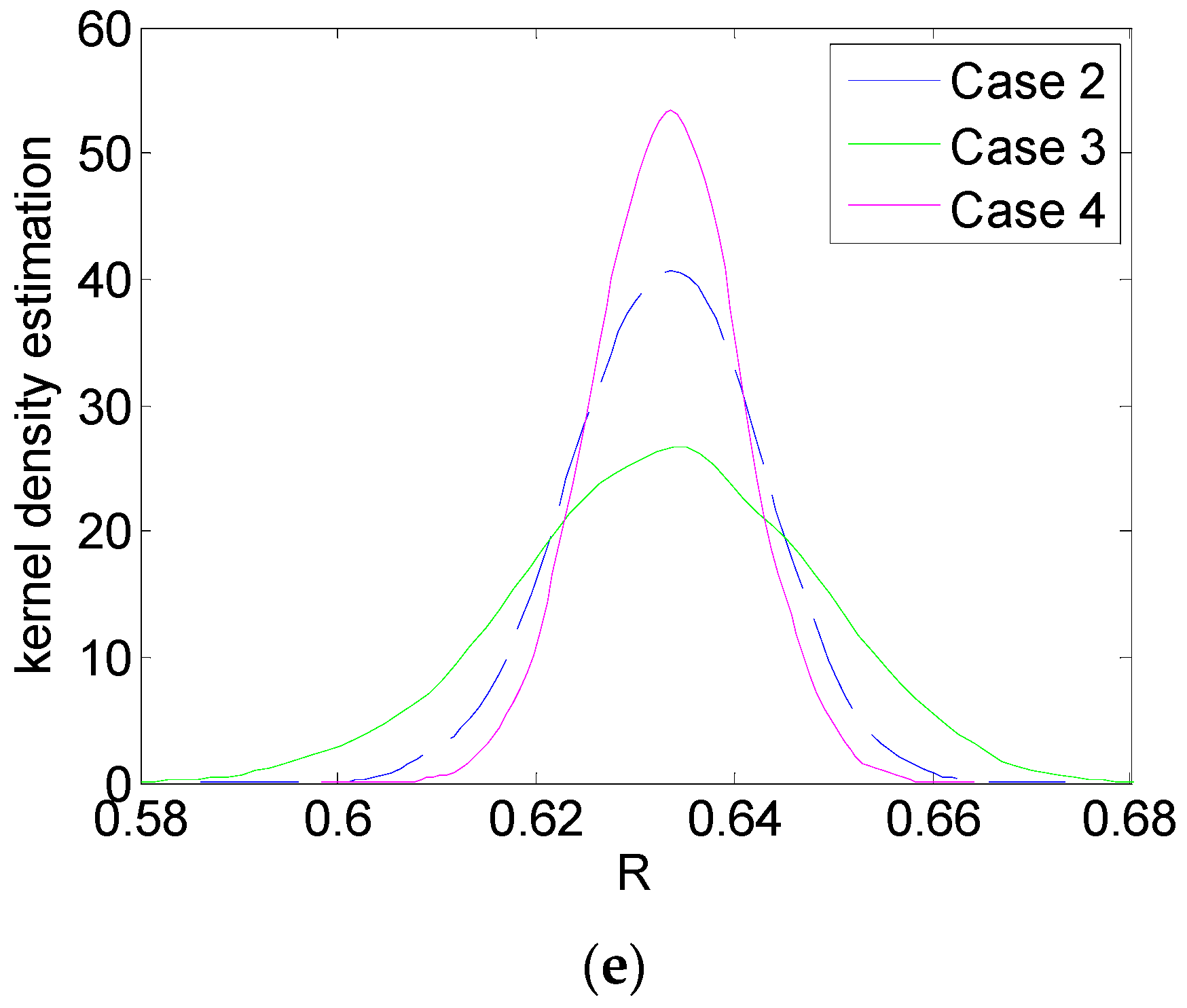
Figure 1. Typical architecture of an AEPS.
Applsci 12 02857 g001
Figure 2. Flow chart of the early reliability design of an aircraft power system.
Applsci 12 02857 g002
Figure 3. System reliability function curve changing with system time.
Applsci 12 02857 g003
Figure 4. A series-parallel system.
Applsci 12 02857 g004
Figure 5. Probability density functions of system reliability for case 1 to case 4. (a) System reliability probability density function in case 1; (b) System reliability probability density function in case 2; (c) System reliability probability density function in case 3; (d) System reliability probability density function in case 4. (e) The comparison of system reliability probability density functions of different cases.
Applsci 12 02857 g005aApplsci 12 02857 g005b
Figure 6. Kernel density function of system reliability after different improvement solutions are applied. (a) Kernel density function of system reliability after solution 1 is applied; (b) Kernel density function of system reliability after solution 2 is applied; (c) Kernel density function of system reliability after solution 3 is applied; (d) Kernel density function of system reliability after solution 4 is applied; (e) Kernel density function of system reliability after solution 5 is applied. (f) The comparison of the kernel density function of system reliability of five solutions.
Applsci 12 02857 g006aApplsci 12 02857 g006b
Table 1. Means and variances of system reliability in four cases (T = 7 h, M = 1000).
Case 1Case 2Case 3Case 4
Mean0.63350.63320.63270.6332
Variance8.7879 × 10−289.0439 × 10−52.3694 × 10−45.7243 × 10⁻⁵
Confidence intervals[0.6335, 0.6335][0.6144, 0.6519][0.6016, 0.6612][0.6182, 0.6477]
Table 2. Importance measure indicators of components in four cases (T = 7 h, S = C = 1000).
Case 1Case 2Case 3Case 4
η 1 2 0.00000.01240.00590.0199
η 2 2 0.00000.01210.02070.0055
η 3 2 0.00000.48650.19050.7713
η 4 2 0.00000.48940.79610.1915
Table 3. Failure rate of each component of the AEPS system.
ComponentFunctionMode of λmode (1/H)Low Limit of λlowerUpper Limit of λupper
TB/GBCurrent Relay, Contactor and Breaker1.33 × 10−51.0 × 10−59.9 × 10−5
GeneratorAC Power Source5.56 × 10−51.0 × 10−59.9 × 10−5
AC BUSDirect power distribution to AC loads5.00 × 10−61.0 × 10−69.9 × 10−6
Table 4. Calculation of the importance of the failure rate of each component of the power supply system (T = 1000 h).
η 1 2 η 2 2 η 3 2 η 4 2 η 5 2 η 6 2 η 7 2 η 8 2 η 9 2 η 10 2 η 11 2
ComponentLGLGBLG BUSBTB1APUG BUSAPU GBAPUGBTB2RG BUSRGBRG
Importance0.0970.13060.38030.36360.00310.00610.00530.00260.00060.00290.0024
Ranking4312756911810
Table 5. Five system reliability improvement/optimization solutions.
SolutionImprovement ComponentImprovement Measures
Solution 1LG BUSReselect component LG BUS of less fluctuation in failure rate with flight environment changes to replace the original one.
Solution 2BTB1Reselect component BTB1 of less fluctuation in failure rate with flight environment changes to replace the original one.
Solution 3BTB1, LG BUSReselect both components BTB1 and LG BUS of less fluctuation in failure rate with flight environment changes to replace the original ones.
Solution 4LG, LGB, BTB1, and LG BUSReselect components LG, LGB, BTB1 and LG BUS of less fluctuation in failure rate with flight environment changes to replace the original ones.
Solution 5No. 5 to No. 11Reselect components of No. 5 to No. 11 which have less fluctuation in failure rate with flight environment changes to replace the original ones.
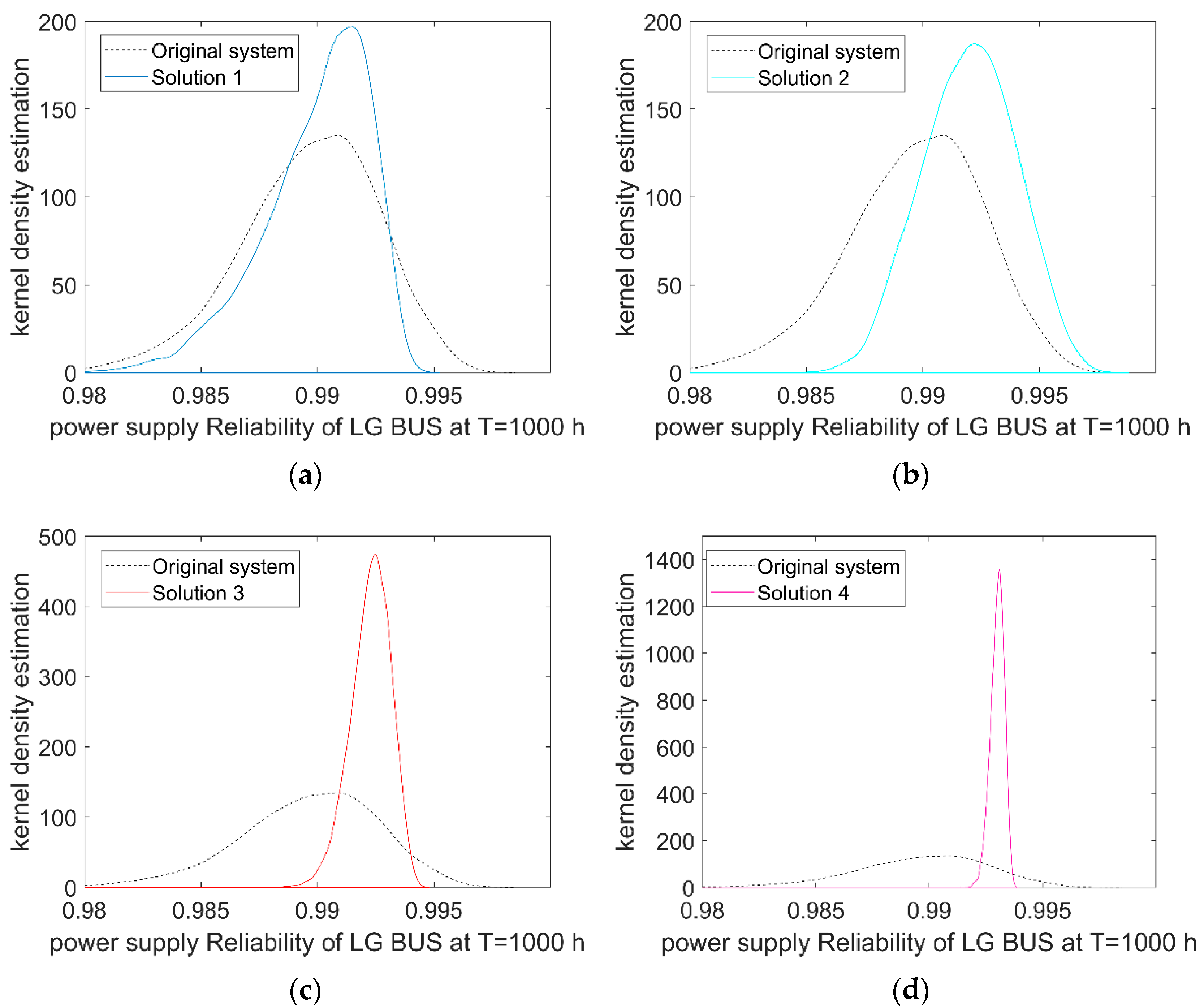
Table 6. System reliability of LG BUS under different improvement schemes (T = 1000 h).
SolutionImportance DegreeMean ValueVarianceConfidence IntervalsReduction DegreeEfficiency Ranking
Original-0.98968.6910 × 10−6[0.9831, 0.9947]--
Solution 10.380.98995.28320 × 10−6[0.9844, 0.9932]39.21%3
Solution 20.360.99205.53452 × 10−6[0.9880, 0.9957]36.32%4
Solution 30.740.99232.29312 × 10−6[0.9904, 0.9937]73.62%2
Solution 40.970.99302.49012 × 10−7[0.9923, 0.9935]97.13%1
Solution 50.0230.99028.39620 × 10−6[0.9841, 0.9951]3.39%5
Publisher’s Note: MDPI stays neutral with regard to jurisdictional claims in published maps and institutional affiliations.

