3.1. Importance Measure Index
In order to reasonably measure the influence of the uncertainty of the failure rate
λ of each component on the power supply reliability of the sink nodes
s given a system time
T, the importance measure index
in Equation (3) can be defined according to the variance decomposition theory [
44,
45].
In Equation (3), the subscript s represents the s-th sink node of AEPS, s = 1, 2, …, Num; the subscript i represents the i-th component in the system, i = 1, 2, …, n; ~i represents the rest components of the system except for component i; represents the vector of the failure rates of the remaining components of the system except for , for example, for a system containing four components, if i = 2, then ; is the proposed importance measure index to measuring the uncertainty contribution of the i-th component failure rate on the uncertainty of the supply reliability of the sink node s. is the unconditional variance of power supply reliability of the sink node s; is the conditional expected value of power supply reliability of the sink node s, and to be specific, it is on the condition that the failure rate of the i-th component is given; accordingly, is the variance of .
3.2. Calculation Method
Based on the Monte Carlo simulation theory [
20,
32], this paper proposed a method to estimating
(
i = 1, 2, …,
n,
s = 1, 2, …,
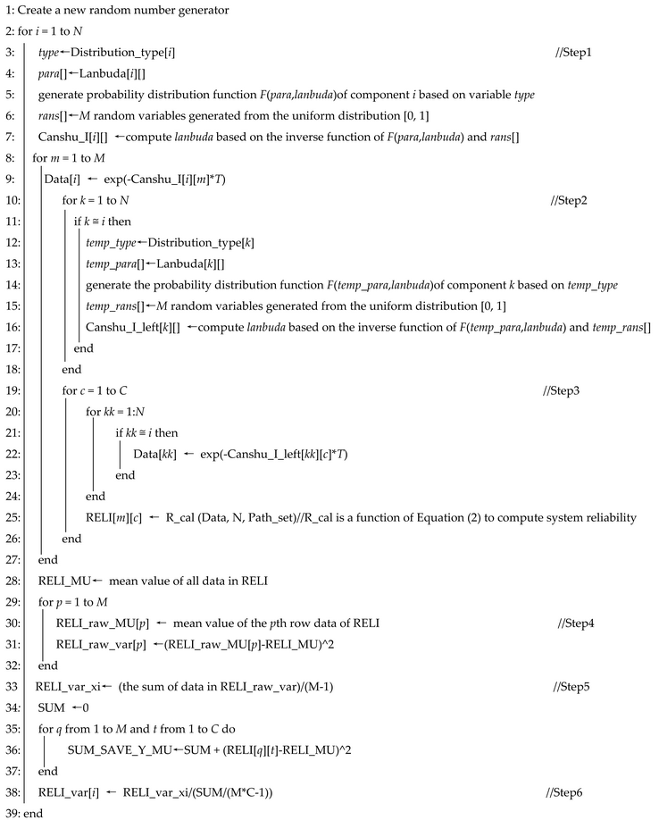
Num), which includes six steps. The pseudocode of the algorithm is shown in Algorithm 1, and the steps are explained below.
Step 1: Establish a failure rate sample vector for component i.
According to the probability distribution function F() that variable obeys, the inverse transformation method is adopted to generate M samples to form the sample vector . Specifically, generate M random variables U1, U2, …, UM from the uniform distribution in the interval [0, 1] first, which is U~Uniform(0, 1). Then, use the inverse distribution function F−1(U) to calculate the random variable : , j = 1, 2, …, M.
Step 2: Establish a component failure rate sample matrix .
Similarly, for
(
j = 1, 2, …,
M) in vector
, use the inverse transformation method to generate sample
(
k = 1, 2, …,
C) from the conditional probability distribution
to form the component failure rate sample matrix
(
j = 1, 2, …,
M), see Equation (4).
In the reliability analysis of AEPS, the failures between different components are generally considered to be independent of each other, so formula is established. In the component failure rate sample matrix , the element is the k-th vector composed of the failure rates of the remaining components of the system under the failure rate . For example, for the power supply bus s, if there are four components that affect its power supply reliability in the system, then for the 2nd component (i = 2), the vector in the proposed matrix is donated as .
Step 3: Calculate the power supply reliability matrix Rs of the sink nodes s.
Substitute the sample point [
,
] of the obtained component failure rate sample matrix into Equation (2) to calculate the power supply reliability
of the sink nodes
s, of which
represents the function with the state of each component in the system as a variable and the power supply state of the sink nodes
s is a dependent variable. It is clear that
(
j = 1, 2, …,
M,
k = 1, 2, …,
C) can form an output matrix
Rs with size
M ×
C;
| Algorithm 1: Importance_Calculation (Lanbuda[][], Distribution_type[], s, Path_set[][], T, RELI_var[]) |
//Input: array Lanbuda with size SN, Distribution_type with size N, Path_sets with size Num N, variable s and T. N is the component number in the MPSs of sink node s. S is the max number of parameters that used to describe the probability distribution of each component’s failure rate, e.g., there are two components in the MPSs of sink node s, and the failure rates of the first and the second component follow lognormal and triangular distributions, respectively, which are described with two and three parameters in separate, so S = 3. The ith element represents the distribution type of component i’s failure rate, and the ith column of Lanbuda stores the probability distribution parameters of node i’s failure rate. Num represents the number of MPSs of sink node s and the ith row of Path_sets stores the components in the ith MPS. T represents system time.
//Output: array RELI_var with size N. Its ith element represents component i’s importance degree that measures the contribution to the uncertainty of node s’s power supply reliability.
![Applsci 12 02857 i001]() |
Step 4: Estimate the value of .
For
j-th row of the output matrix
Rs,
j = 1, 2, …,
M, use Equation (5) to calculate the mean reliability.
The term indicates the expected value of the power supply reliability of the sink nodes s when the failure rate of the component i takes the value .
Step 5: Estimate the unconditional variance of power supply reliability and the variance of .
For the power supply reliability of sink nodes
s, estimate its value of expectation using Equation (6). Then, with the help of Equation (7), calculate the estimation value
of variance
. Finally, use Equation (8) to calculate the estimation value
of variance
:
Step 6: Compute the estimation value of the proposed importance measure index .
Substitute the results of Equations (7) and (8) into Equation (9), the importance measure index of component
I, which can quantify its failure uncertainty contribution to the power supply reliability uncertainty of the sink node
s, is estimated.
The physical meaning of the six steps is explained as follows. First, each element in
j-th row of the matrix
stands for the failure rate sample of the remaining components when the
i-th component takes the value
. Accordingly, for the power supply reliability matrix
Rs obtained through the matrix
, each element in its
j-th row represents a possible value of the power supply reliability of sink node
s when the failure rate of component
i takes the value
, and the mean value of the
j-th row is
by averaging
C possible values of the row. In addition, according to the law of large numbers, as the value of
C increases,
will surely converge to the expectation
; moreover, when the two samples
and
of the failure rate of the
i-th component are the same, the mean value
and
tend to be the same as
C increases. That is to say, for the row mean value
,
of the matrix
Rs, the numerical difference between them is mainly caused by the different failure rate values of component
i. Therefore, the variance
calculated by Equation (7), quantifies the degree of dispersion of the power supply reliability of the sink nodes
s induced by the dispersion of the failure rate of the component
i. Since the uncertainty of output propagated from input can be measured with the variance of the output variable [
44], the variance computed by Equation (7) has the ability to quantify the uncertainty of the failure rate of component
i on the contribution of the power supply reliability uncertainty of the sink node
s. Furthermore, because the variance calculated by Equation (8) is based on all the elements in the matrix
Rs and the matrix includes all the possible values of the power supply reliability of the sink node
s, the obtained variance
is a measurement that quantifies the failure uncertainty contribution of all the components to the uncertainty of the power supply reliability of the sink node
s.
In summary, first, the ratio of variance to variance calculated by Equation (9) essentially quantifies the ratio of the uncertainty that the i-th component contributes to and the whole uncertainty that all the components contribute to in theory; and according to the law of large numbers, with , holds. This means that if the simulation results obtained by the proposed method satisfies the convergence condition: , it indicates that the sampling sizes M and C are reasonable, otherwise, the sampling size needs to be increased until the convergence condition is met. Second, from the index definition of Equation (3) and the above explanation, it can be seen that this index value varies in the range [0, 1]. Furthermore, the higher the index value of one component, the greater the influence of the uncertainty of the component’s failure rate on the uncertainty of system reliability, and vice versa. Therefore, the index can help designers identify which components are more important to the system to reduce the system reliability uncertainty, and the quality and performance of these components with a higher index can be prioritized to be improved. Conversely, improving components with lower index will not achieve better results. Algorithm 1 shows the pseudocode of the proposed algorithm for computing the importance degree.


