Abstract
Recently, deep-learning-based image super-resolution methods have made remarkable progress. However, most of these methods do not fully exploit the structural feature of the input image, as well as the intermediate features from the intermediate layers, which hinders the ability of detail recovery. To deal with this issue, we propose a gradient-guided and multi-scale feature network for image super-resolution (GFSR). Specifically, a dual-branch structure network is proposed, including the trunk branch and the gradient one, where the latter is used to extract the gradient feature map as structural prior to guide the image reconstruction process. Then, to absorb features from different layers, two effective multi-scale feature extraction modules, namely residual of residual inception block (RRIB) and residual of residual receptive field block (RRRFB), are proposed and embedded in different network layers. In our RRIB and RRRFB structures, an adaptive weighted residual feature fusion block (RFFB) is investigated to fuse the intermediate features to generate more beneficial representations, and an adaptive channel attention block (ACAB) is introduced to effectively explore the dependencies between channel features to further boost the feature representation capacity. Experimental results on several benchmark datasets demonstrate that our method achieves superior performance against state-of-the-art methods in terms of both subjective visual quality and objective quantitative metrics.
1. Introduction
As one of the crucial technologies in the computer vision field, image super-resolution (SR) aims to reconstruct latent high-resolution (HR) image with bountiful details from one or more available low-resolution (LR) images [1], and it has widely used in medical imaging [2], video surveillance [3], satellite images [4], etc. However, SR is essentially an ill-posed inverse problem since multiple HR solutions may correspond to the same LR input [5].
At present, with the development of the high-profile deep convolution neural networks (CNNs), deep-learning-based SR methods have received a great deal of attention for their fantastic exhibition. Numerous specialists have proposed many effective and brilliant hand-crafted models to improve the super-resolution performance by superimposing a large number of modules to extract features from different levels, such as [6,7,8,9,10,11,12,13]. Although these methods can boost the feature representation capability, they make the network increasingly complex, which prompts the problem of gradient exploding and vanishing. As we know, the training difficulty can be alleviated by exploiting the residual block [14], but such methods [6,7,8,9,10,11,12,13] ignore the feature correlation of the intermediate layers. Consequently, the features in the intermediate layers cannot be used straightforwardly and viably, and some extremely representative residual features are just being used locally, which causes the network to suffer from performance bottlenecks. Meanwhile, the study in [15] has revealed that investigating the interdependence of channel features can likewise be integrated into the network to upgrade the feature representation ability. Nonetheless, most previous CNN-based SR methods assign the same weights to each channel feature, resulting in the loss of significant details of reconstructed images. In addition, there are numerous CNN-based SR models that directly learn the mapping between LR and HR images by minimizing the loss function. However, due to the lack of prior knowledge of the image, these methods are difficult to reconstruct clear high-frequency details. Hence, in the SR task, not only image details need to be recovered effectively, but also the original structure inherent in an image needs to be preserved as much as possible [16].
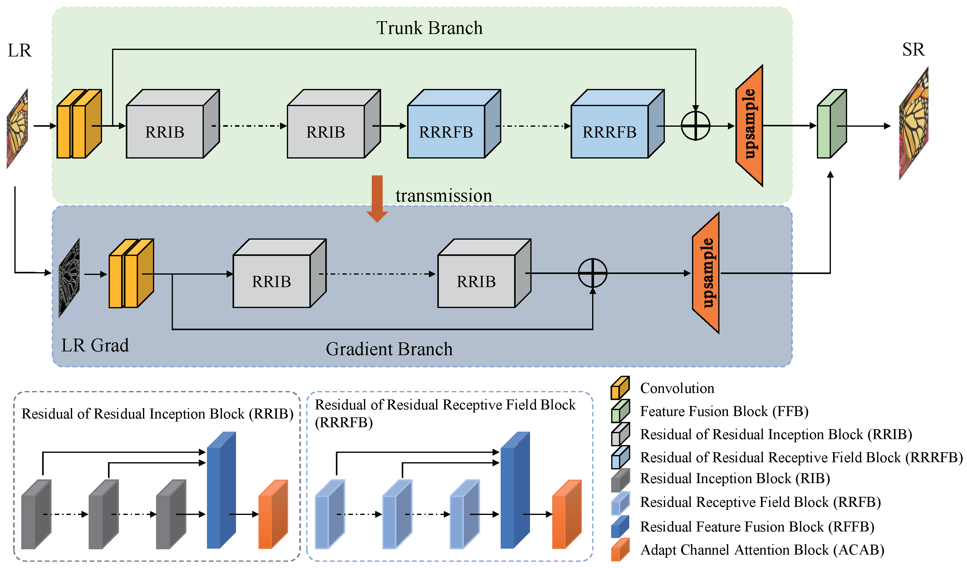
To solve the issues mentioned above, we propose a gradient-guided and multi-scale feature network for image super-resolution (GFSR), which fuses the extracted multi-scale intermediate features and treats gradient feature map as structural prior to guide the image super-resolution process to recover as many details as possible. Considering that the gradient map is able to adequately reveal the sharpness information of local region of an image, and this sharpness information can be transformed into the structural information, we attempt to utilize the gradient map to guide the image super-resolution process. Simultaneously, the SR task can essentially be regarded as a color-filling problem that provides strong clues for LR images after the image structure information is acquired [16]. Consequently, to better preserve the original image structure, the designed GFSR model contains the trunk branch and the gradient one, as shown in Figure 1. On the gradient branch, the gradient map of the LR image is first extracted and converted to the gradient map of the HR image, and then the obtained HR gradient features are coordinated into the trunk branch through a feature fusion block (FFB) to provide effective structural prior for the image super-resolution process.
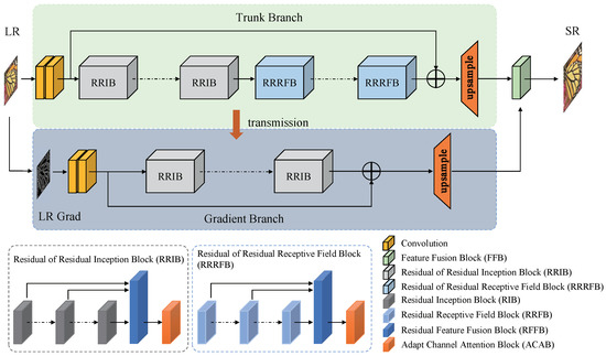
Figure 1.
Network structure of the proposed GFSR. The network is divided into two branches, the trunk branch for extracting the intermediate features from the LR image, as shown in the upper part of this figure, and the gradient branch for extracting the gradient map of the LR image, as shown in the lower part of this figure. Notably, the intermediate features extracted on the trunk branch are propagated to the gradient branch to reduce the number of parameters; at the same time, the gradient features extracted on the gradient branch are propagated to the trunk branch through a feature fusion block to guide the super-resolution process.
To explore more abundant features from different layers, we design two different multi-scale feature extractors, namely residual of residual inception block (RRIB) and residual of residual receptive field block (RRRFB), as shown in Figure 1. Both feature extractors utilize multi-scale convolution kernels with parallel structures to replace single-scale convolution kernels to extract intermediate features at various scales. It is worth noting that the proposed multi-scale convolution module is able to simultaneously extract coarse and fine features from the input LR image without increasing the network depth, so as to facilitate more effective learning of the complex mapping relationship between LR and HR counterparts [17,18,19]. Then, to fully utilize the extracted features, we propose an adaptive weighted residual feature fusion block (RFFB) to fuse features extracted from different intermediate layers of the residual block, which can reduce the network training difficulty, and additionally generate more beneficial features simultaneously. Existing studies [14,15] show that there exist some important inter-dependencies between channel features, and the feature representation ability of the model can be viably enhanced by fully exploring and exploiting such interdependencies. To this end, an adaptive channel attention block (ACAB) [20] is incorporated into our GFSR model to highlight the informative features in different channels, so as to further promote the feature utilization.
In general, the primary contributions of this paper are as follows:
- We propose a gradient-guided and multi-scale feature network for image super-resolution (GFSR), including a trunk branch and a gradient branch, and extensive experiments demonstrate that our GFSR outperforms state-of-the-art methods for comparison in terms of both visual quality and quantitative metrics.
- The gradient feature map is extracted from the input image and used as structural prior to guide the image reconstruction process.
- Two effective multi-scale feature extraction modules with parallel structure (i.e., RRIB and RRRFB) are proposed to extract more abundant features at different scales.
- An adaptive weighted residual feature fusion block (RFFB) is proposed to exploit the dependency of image contextual feature information to generate more discriminative representations.
The organization of this paper is as follows. In Section 2, we summarized the related works. In Section 3, we described the proposed GFSR in detail. In Section 4, we analyzed the experimental results and compared the results with the recent state-of-the-art SR methods. Finally, we concluded this paper in Section 5.
2. Related Works
Recent CNNs have been widely used for SR tasks and achieved considerable performance due to their robust feature representation ability. In this section, we first briefly introduce CNN-based SR methods, and then present residual network, attention mechanism and gradient feature that are closely related to the proposed model.
2.1. CNN-Based SR Models
CNNs have achieved great success in SR tasks. Lai et al. [21] proposed a deep Laplacian pyramid network (LapSRN), which gradually predicts the sub-band residuals of HR images in a coarse-to-fine manner, and efficiently restores the reconstructed images by the predicted sub-band residuals. Zhang et al. [22] designed a deep plug-and-play super-resolution model (DPSR), which utilizes an iterative optimization scheme based on variable splitting to estimate the blurred kernels to cope with the challenges of different degradation models. Huang et al. [23] exploited a detail-fidelity attention network (DeFiAN), which employs the proposed Hessian filtering to extract the high-frequency features, and improves the extracted Hessian features through a dilated encoder-decoder mechanism as well as a distribution alignment unit, respectively, to achieve high-quality reconstruction. Wang et al. [24] developed a degradation-aware SR model (DASR), which introduces a degradation-aware module to discriminate different degradation models by learning different feature representations, thus achieving good super-resolution performance.
As the network depth increases, the number of model parameters increases dramatically. To reduce computational complexity while improving super-resolution performance, Zheng et al. [25] developed an information distillation network (IDN), which effectively utilizes the local long and short-path features to enhance the quality of reconstructed images by combining an enhancement unit with a compression unit. Further, to improve the performance of IDN, Zheng et al. [26] proposed an information multi-distillation network (IMDN) by adopting the residual block, which utilizes the proposed adaptive cropping method to achieve super-resolution restoration at arbitrary scales. In addition, to decrease the computational cost, Li et al. [27] propose a linearly-assembled pixel-adaptive regression network (LAPAR), which transforms the conventional learning of LR to HR mappings into a multiple predefined regression task on linear filter coefficients. Wang et al. [28] proposed a sparse mask SR model (SMSR) to boost the inference efficiency by exploring the sparsity in SR tasks. SMSR determines significant and redundant regions by spatial mask learning and channel mask learning, respectively, and maintains superior performance while skipping redundant computations.
2.2. Residual Network
Existing studies [6,7,8,9,10,11,12,13,29] have indicated that great features with stronger representation ability can be yield as the network depth increases. However, deep networks built in such way may suffer from gradient vanishing or exploding, resulting in network convergence difficulty and poor optimization. For the sake of resolving this issue, He et al. [29] proposed the residual network (ResNet), which introduces cross-layer jump connections and adds identity mapping of shallow features to make the forward and backward propagation of information without a hitch, thereby promoting the feature representation ability of the network effectively. Currently, ResNet has been extensively exploited in CNN for various computer vision tasks.
As the earliest deep learning based SR method, SRCNN [30] was a simple structure network with fewer convolutional layers, which causes the inadequate feature extraction capacity, resulting in unsatisfactory super-resolution performance. Inspired by ResNet, the residual network was incorporated into the super-resolution model to develop the deeper network to recover more abundant details [6,7,8,9,10,11,12,13,14,15], such as SRResNet [7], EDSR and MDSR [8], DRCN [9], RCAN [15], etc. To fully exploit shallow and deep features, Kim et al. [6] proposed an accurate image super-resolution using very deep convolutional networks (VDSR), which fastly propagates the low-level features to the high-level layers and increases the feature propagation efficiency. However, for deeper networks, the problem of gradient exploding or vanishing may not be effectively solved by using the global residual structure simply. For this reason, many SR methods [10,11,12,13] jointly exploit local and global residual features. Such methods can not only make full use of the image features, but also solve the problem of feature disappearance during transmission, thereby enhancing the quality of super-resolving images performance generally. To further improve the feature utilization, Liu et al. [14] proposed a residual feature aggregation network (RFAN), which aggregates the local features extracted from several residual blocks through jump layer connections to generate more representative features, thereby achieving considerable super-resolution performance.
2.3. Attention Mechanism
Attention in human vision refers to the part of the human visual system (HVS) that adaptively measures visual information and focuses attention on salient areas [31]. Notably, not all the features assume an imperative part for the expectant reconstructed image in SR tasks lately. However, most recent SR methods treat all channels or spatial locations equally. The study in [15] shows that, in some cases, selectively focusing on a few important features of a specific layer can bring considerable improvements to the reconstruction performance of the model. Therefore, the SR methods based on the attention mechanism have received increasing attention [14,15,32,33,34,35].
Lu et al. [32] developed a compact channel attention mechanism in the recursive unit to adaptively recalibrate the input channel features to flexibly adjust the weights of different channel features, thereby promoting the reconstruction quality to a certain extent. Zhang et al. [15] introduced the channel attention mechanism into ResNet and assigned different weights to each channel feature according to the different contribution of channel features to the super-resolution performance, which greatly enhanced the detailed information of the reconstructed image. This mechanism mainly utilizes a global pooling operator to extract channel feature statistics information, which can be named first-order channel attention. On the basis of the first-order channel attention, Dai et al. [33] proposed a second-order attention network (SAN), which endeavors second-order feature statistics to exploit more remarkable representations. However, considering that it is difficult to weigh the features from multi-scale layers by using the channel attention mechanism alone, Niu et al. [34] proposed a holistic attention network (HAN) for image super-resolution. HAN regards channel features from different layers as responses of specific classes and explores the channel features between different layers, which accelerates the feature extraction ability. In addition to the potential relevance of channel features, the potential dependence of spatial features has also attracted wider attention. For example, Niu et al. [34] also explored the internal relevance of spatial features and proposed a channel-spatial attention module to boost the reconstruction performance. To adequately coordinate the extracted feature information, Liu et al. [14] proposed an enhanced spatial attention module to make the extracted features focus on the significant spatial content. Furthermore, Zhao et al. [35] proposed a pixel attention based network (PAN) for image SR, which explores the dependence between the long-range space around each spatial location and the channel through adopting a self-calibration method, thereby improving the reconstruction accuracy.
2.4. Gradient Feature
In the past few decades, the prior-based image restoration methods have achieved remarkable results. Since the edge is one of the most important image features, the edge prior has also become one of the most effective image priors. Xie et al. [36] utilized edge prior to guide image super-resolution, which effectively enhanced the edge details of the reconstructed image. At the same time, structure prior has also received more and more attention because it is able to provide effective clues for the estimation of high-frequency details. Sun et al. [37] obtained the image structure information by extracting gradient features, and then used the structure prior to guide image super-resolution to improve restoration ability of high-frequency details. Yan et al. [38] proposed a combination of multiple gradient description models and estimated the parameters of multiple gradient descriptors at different resolutions to obtain descriptions of different edge contours to obtain effective gradient contours. These methods are mainly based on statistical correlation, observing the parameter estimation from LR to HR to obtain edge estimation parameters to model. However, such methods are often very complicated and inefficient.
Currently, for the most popular deep-learning-based SR methods, some models also explore and exploit image priors in the network to promote super-resolution performance. Yang et al. [39] introduced the image edge structure to CNN for the first time and proposed the DEGREE model. However, DEGREE directly uses the LR map obtained by Bicubic, which may introduce additional noise, resulting in poor super-resolution performance. To boost the restore ability of details, Jiang et al. [40] incorporated gradient feature into the GAN model, and used the gradient map as a structure prior to guide image super-resolution, thereby alleviating the geometric distortion and artifact noise generated by the GAN model.
3. Proposed Network
There exist some problems for most CNN-based SR methods, for example, the structure information of the image cannot effectively be exploited, a single-scale convolutional kernel is utilized solely to separate features, there is no viable fusion mechanism between adjacent feature extraction modules, and each channel feature is dealt with similarly. To tackle the above issues, we propose a gradient-guided and multi-scale feature network for image super-resolution (GFSR) to reconstruct as much detailed information as possible.
In this section, we first present the overall framework of the network, and afterward describe the gradient branch, multi-scale convolution unit, residual feature fusion block, and the adaptive channel attention block used in detail.
3.1. Network Structure
As can be seen from Figure 1, our GFSR consists of two branches, including the trunk branch and the gradient one. On the trunk branch, M Residual of Residual Inception Blocks (RRIB) and N Residual of Residual Receptive Field Blocks (RRRFB) form a deep feature extraction module to acquire the deep features of the input image, and a feature fusion block (FFB) is designed to integrate the gradient features produced on the gradient branch to the trunk branch to generate the reconstructed images. On the gradient branch, P RRIBs are used to extract features from the LR gradient map and receive the intermediate features at different levels produced on the trunk branch. Finally, the extracted gradient features from all RRIBs are used as an essential structural prior to guide the super-resolution process.
On the trunk branch, the shallow feature of the input image can be obtained by two cascaded 3 × 3 convolutional (Conv) layers,
where stands for the shallow feature extraction function.
Then, is sent to the deep feature extraction module consisting of M RRIBs and N RRRFBs to further acquire the corresponding deep feature. Let and respectively denote the functions of RRIB and RRRFB, and let denote the features obtained by the upsampling module, then we can get,
where represents the output features obtained by M RRIBs, represents the output features obtained by N RRRFBs, ⊕ stands for the element-addition operation, and represents the upsampling operation.
On the gradient branch, the gradient map of the input image is first calculated through the gradient function , which is then passed through a series of modules (i.e., two Convs, P RRIBs, and an upsampling module) to obtain the corresponding gradient features ,
where denotes the shallow feature of the gradient map obtained by two cascaded Convs, and denotes the deep features obtained by P RRIBs.
Finally, the gradient features produced on the gradient branch are fused to the trunk branch to generate the reconstructed image ,
where denotes the feature fusion block.
3.2. Gradient Branch
To effectively exploit the gradient features of LR images, we design a gradient branch structure. On the gradient branch, the gradient feature map of the LR image is used to estimate the one of the HR image, which is used as structural prior information to guide the super-resolution process.
The gradient map is generally acquired through exploring the difference between adjacent pixels in the horizontal and vertical directions,
where , denotes the coordinate of the pixels, represents the gradient function, and represents the second norm. Considering that the gradient map is close to zero in most regions of an image, it facilitates CNN to pay more attention to explore the spatial relationship of the image structure, thereby estimating an approximate gradient map for the SR image.
As shown in Figure 1, several intermediate-level features on the trunk branch are sequentially propagated to the gradient branch, so the output of the gradient branch not only contains the image structure features, but also contains abundant detail and texture features. Such a design method is not only effectively supervised to recover the gradient map, but also significantly reduces the number of parameters of the gradient branch. At the same time, since the gradient map is able to directly reveal whether a particular region of the image is sharp or smooth, we fuse the gradient features obtained from the gradient branch to the features on the trunk branch to guide the super-resolution process. Specifically, in our network, the features from the 5th, 10th, 15th, and 20th modules in the trunk branch are propagated to the gradient branch, and then the gradient features obtained by the gradient branch are integrated into the trunk branch.
3.3. Multi-Scale Convolution Unit
To improve the feature representation ability of the network, a common method is to design a very deep network with tremendous convolutional layers to explore more abundant features. Although this method can improve network performance to a certain extent, it also brings other problems. On the one hand, the extending of the network depth is accompanied by a continuous expansion in the number of parameters, which may prompt overfitting in the case of inadequate training data. On the other hand, a network with an incredible number of layers implies higher computational complexity and is prone to bring in gradient exploding or vanishing, making network optimization difficult. Fortunately, the GoogLeNet [41] model solves these problems well. The critical thought of the Inception is to build a dense block structure. It utilizes multi-scale convolution kernels to acquire the feature map, and then combines the output of several branches to the following layer. The structure accelerates both the qualities and the resilience to scale without increasing the network depth of the network, thus improving the capability of feature extraction.
For the RIB structure, different from the original Inception module, we removed the pooling layer. Since the max-pooling operation extracts the maximum value of the feature map in a certain area to generate the representative salient features in the area, which may result in the loss of a large amount of detail features. Thus, the pooling operation is often fatal for SR tasks. For example, a max-pooling operation may cause the feature map to losing nearly of the important information. For low-level tasks such as image super-resolution, the feature information of each pixel is very important. Consequently, we directly use the stepping convolutional layer to replace the pooling layer.
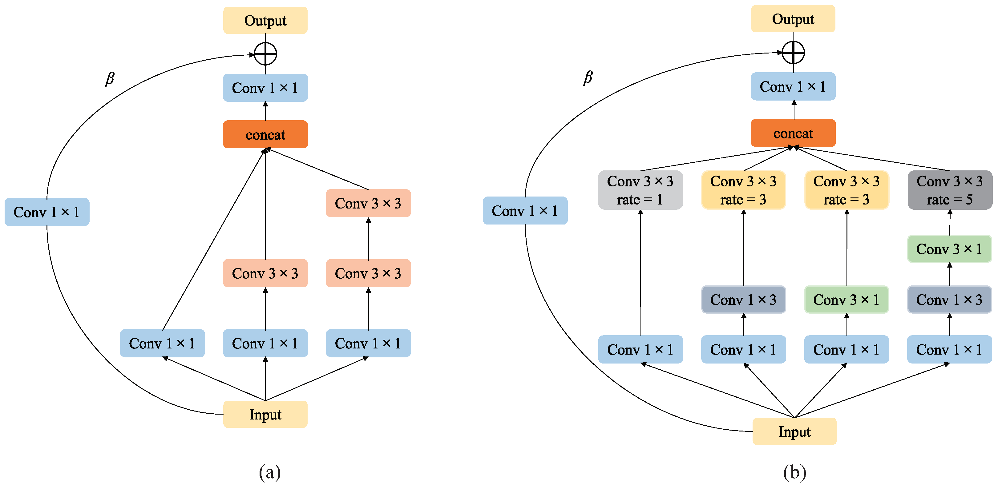
For the SR task, we propose a multi-scale convolution unit with a parallel structure to extract the receptive field features of different scales to recover as many image details as possible. Specifically, we first assemble convolution filters of various scales into the network, such as , , . However, a larger-scale convolution kernel incurs higher computational costs and increases the time complexity. Consequently, in our network, we use small-scale filters instead of large-scale ones to minimize the number of parameters [42,43]. In fact, in our network, only and scale convolution filters are used, and the scale filter is replaced by two cascaded scale filters. Ref. [42] has proved that the features extracted by filters with a scale larger than are typically weak as the filter with a scale larger than can generally be simplified to a set of filters with a scale of , and the parameter of two cascaded scale filters is only 18/25 of the parameter of a single scale filter. As shown in Figure 2a, our RIB (Residual Inception Block) employs the multi-branch structure with different scale convolution kernels to correspond to different sizes of receptive fields, and the scales of the convolution kernel on the three branches are , and , and a set of cascaded , respectively. In this way, more features could be learned, and then the features of the three branches are fused to obtain the representative feature.

Figure 2.
Multi-scale convolution unit. (a) is the RIB used in the front layers of the network, (b) is the RRFB used in the posterior layers of the network.
In addition, Ref. [42] also proved that asymmetric convolution kernels [44] could be used to replace conventional symmetric convolution kernels. In certain situations, asymmetric convolution kernels can learn more representative features than symmetric convolution kernels, and reduce computational complexity without loss of accuracy. Furthermore, the receptive field of the human eye is related to the eccentricity of the retina center [45], and the size of the receptive field varies with the eccentricity, which can be controlled accessibly by the dilated convolution to achieve adjusting the size of the receptive field. Therefore, the asymmetric convolution kernel and the dilated convolution are separately introduced into the proposed multi-scale convolution unit to enhance the ability of feature extraction.
Importantly, it was proposed in Ref. [42] that the asymmetric convolution unit has a lackluster performance to be placed in the front of the architecture, while more suitable to be placed in the middle and subsequent layers of the network to strengthen the expression ability. We accept the proposal to placing it in the appropriate place of the middle and subsequent layers in our architecture. In our proposed model, the RRFB (Residual Receptive Field Block) model is utilized for posterior-layer feature extraction, which can extract abundant detail features, especially texture and edge features. As appeared in Figure 2b, the RRFB model we exercised is improved from Figure 2a. Specifically, we utilize a set of and asymmetric convolution kernels rather than the convolution kernels referenced previously. Meanwhile, we also introduce dilated convolution at the end of each branch structure to adjust the size of the receptive field of feature extraction for obtaining excellent reconstruction performance. Finally, the features extracted from each branch are merged to obtain the final feature representation.
To make the extricated includes more expressive, we fuse the residual structure in RIB and RRFB respectively, and assign weights to the input features.
3.4. Residual Feature Fusion Block
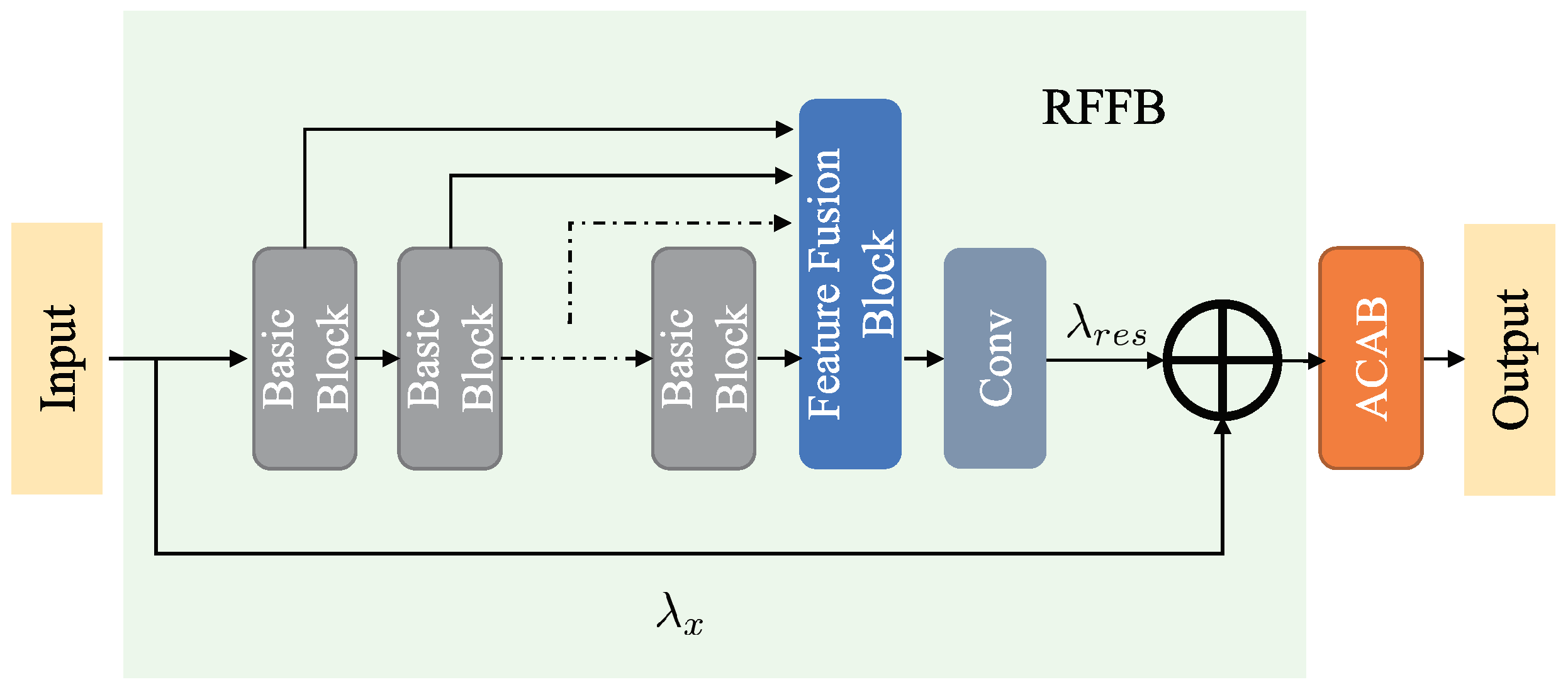
Inspired by the residual network, we design an adaptive weighted residual feature fusion block (RFFB) to solve the low relevance of context information. As shown in Figure 3, our RFFB consists of multiple basic blocks for feature extraction and a local residual feature fusion block. To encourage exploration of the dependencies between the residual channel features, we add a local adaptive channel attention block (ACAB) after the RFFB module. ACAB will be presented in detail in Section 3.5.
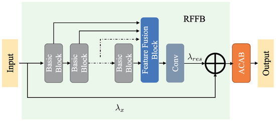
Figure 3.
Residual feature fusion block (RFFB), including several basic blocks for feature extracting and a local residual feature fusion block for fusing the features from different basic blocks.
A traditional residual module stacks a series of feature modules to construct a deep network, so the identity features must go through a long path connection to merge with the residual features, and then propagate the merged features to the subsequent feature extracting block. Thusly, such a design method just yields complex features and does not take full advantage of the neat features extracted from each module, bringing about very localized utilization of features in the process of network learning. More importantly, the contextual information of the image may be lost and its relevance cannot be well expressed.
The residual feature fusion block is designed to fuse the feature information learned from all the feature extraction modules as much as possible. However, simply stacking all the feature information directly together will accumulate an excessive number of features, bring a considerable number of parameters for the network and dramatically increment the difficulty of training. For the sake of solving the above problem, we must adaptively fuse local features obtained by each feature extraction module first and then propagate them to the subsequent layer of the structure. Inspired by MemNet [46], we introduce a convolutional layer after the feature fusion block (FFB) to adaptively adjust the number of output features. As shown in Figure 3, the residual features of B Basic Blocks (such as RIB and RRFB are introduced in Section 3.1) are transferred directly to FFB, then a convolutional layer is designed to reduce the dimension of the feature to the same dimension as the input features, and finally, the output of RFFB is the result of accumulating the identity feature and fusion feature by performing the element addition operation. Assuming that and are the input and output of the m-th RFFB module, and represents the output of the B-th Basic Block of the m-th RFFB module, we can obtain
where denotes the residual feature fusion function, and denotes the Relu activation function.
To fully exploit the expressive power of residual features, as shown in Figure 4, Jung et al. [47] proposed a weighted residual unit (wRU) to generate the weight of the different residual units by wSE(weighted Squeeze-and-Excitation) module. Even though this method improves the presentation of the residual unit, it introduces additional parameters and computational overhead for generating weights. Inspired by wRU, we expect to develop an adaptive weighted residual unit to adaptively learn the weights of residual features. As shown in Figure 3, and are learnable parameters. In our network, their initial values are both set to one, and their values are updated through continuous iterative learning.
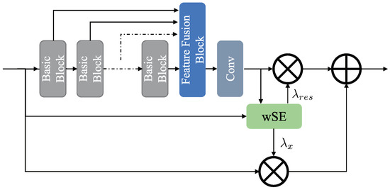
Figure 4.
wRU module, the wSE module is used to generate weight values for different features.
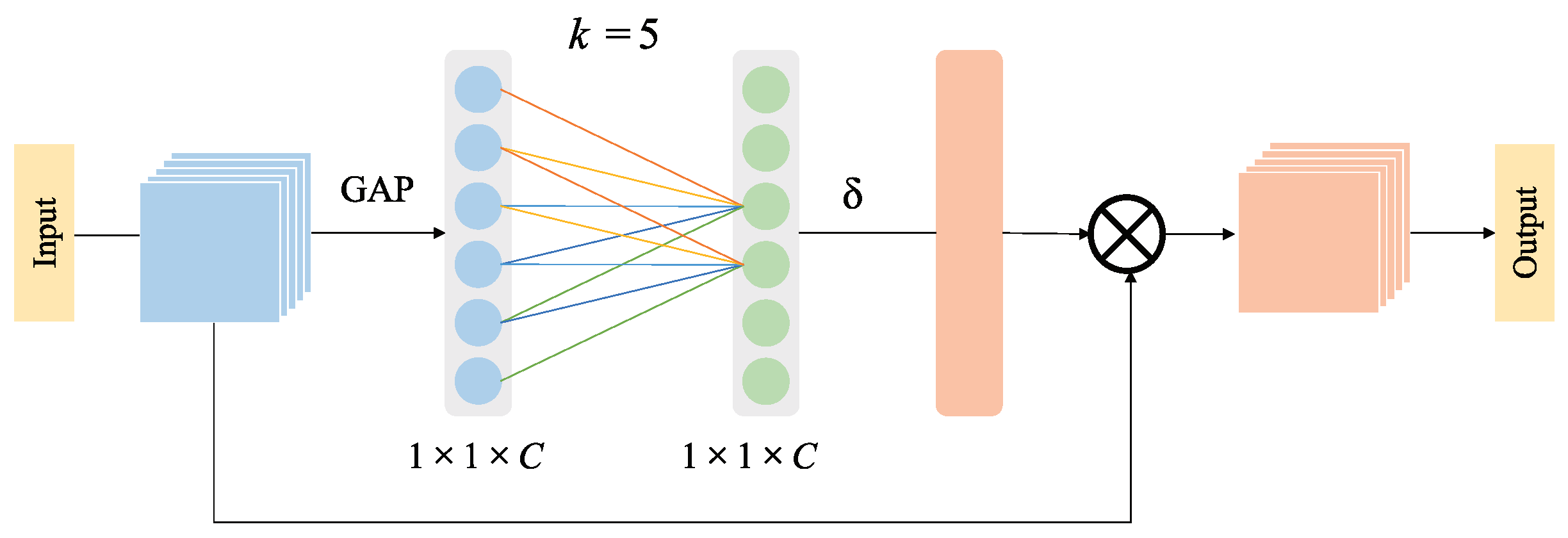
3.5. Adaptive Channel Attention Block
Previous studies [15,33] have revealed that the super-resolution performance can be further improved by incorporating the channel attention mechanism into the SR model. Specifically, the feature representation ability of the CNN model is maximized by assigning different attention degrees to the different channel features.
Inspired by SENet [48], RCAN [15] incorporates the channel attention mechanism into its model and performs the dimensionality reduction operation on feature channels, which effectively improves the visual quality of the reconstructed image and viably diminishes the complexity of the model. Unlike SENet, which performs the fully connected operation on all channels, RCAN only performs fully connected on channels obtained through dimensionality reduction. As pointed out in Ref. [20], the dimensionality reduction operation destroys the direct correlation between the channel and its weight, and the acquired channel attention dependences are wasteful and useless. In order to address the adverse impacts of dimensionality reduction operations on channel attention, we integrate the adaptive channel attention block (ACAB) into the proposed network to explore the correlation dependencies between channel features without pulverizing the primitive relationship between channels. As we all know, the relationship of pixels in an image is identified with the distances among pixels, hence we can infer that the relationship between channel features is additionally equivalent: the great dependence can be found between the adjacent channels, and the dependence relationship is gradually decreasing with the increasing distance of channels. Moreover, Ref. [20] also revealed that the trend of frequency in different images is fundamentally similar in the same convolutional layer, and expresses a robust local periodicity. Therefore, correlation calculations are only performed on the adjacent k channels are in the ACAB.
As shown in Figure 5, ACAB is composed of a global average pooling layer, the nearest neighbor fully connected module, and a channel feature representation layer. Here, the nearest neighbor fully connected module only connects the k nearest channels to investigate the relationship between channels.
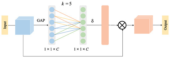
Figure 5.
Adaptive Channel Attention Block.
Based on the above-mentioned analysis, we can roughly get the channel attention weight of the whole image by exploring the relationship between adjacent k channels. The weight of the i-th channel of the feature can be acquired as follows:
where represents the Sigmoid activation function, represents the parameter of the convolution kernel corresponding to , and represents the set of k adjacent channels of .
To further boost the super-resolution performance, all channels share weight information, and then the amount of parameters can be reduced to , as:
where C is the channel number.
Since the adaptive channel attention is to fittingly obtain cross-channel information, it is incredibly necessary to determine the range of channel interaction k. From the previous analysis, we can see that k should be a certain mapping relationship to C,
As the linear mapping relationship has certain limitations, and the number of channels in the SR model is normally a multiple of 2 to further raise the flexibility of the model, the mapping relationship in Equation (14) can be represented as an exponential function with base 2:
Consequently, according to the given C, k can be calculated,
where denotes the nearest odd number of x. Furthermore, the information interaction of cross-channel features can be implemented by using a one-dimensional convolution, that is, a convolutional layer with a convolutional kernel size of k, and it is known that a convolution kernel with an odd size is more competitive than the one with an even size in separating the features, so the value of k is generally taken to be an odd number. Considering that the number k of feature channels is generally selected to be 64 dimensions in most SR models, we also set the feature channel number to 64. Then, k can be calculated according to Equation (16), i.e., .
4. Experimental and Analysis
This section will introduce the database and relevant metrics utilized in the experiments in the first part. Then the experimental details are detailed, followed by relevant ablation experiments to exhibit the adequacy of the proposed module. Finally, we contrast the proposed method with several state-of-the-art SR methods in terms of subjective visual quality and objective quantitative metrics.
4.1. Datasets and Metrics
To train the proposed GFSR, DIV2K [49] is selected as the training dataset, which includes 800 2K training images and 200 validation images. To guarantee the objectivity of our experiments, four commonly benchmark datasets including Set5 [50], Set14 [51], BSD100 [52] and Urban100 [53] are employed for testing. We first convert the obtained reconstructed images into YCbCr space and then calculate the corresponding PSNR [54] and SSIM [55] metrics on the Y channel. It is worth noting that the higher metric means the better super-resolution performance.
4.2. Experimental Details
During training, we perform bicubic downsampling on 800 HR images in the DIV2K set to obtain the corresponding LR images. In our experiments, we enhance the generality of the training images by random horizontal flipping and rotation. The batch size is set to 16, and randomly cropped the LR image into patches as input. Our training is optimized using the Adam [56] optimizer with , , , and [57] is used for loss. In practice, , , , and . Our GFSR has been executed on the PyTorch [58] framework and trained to utilize an NVIDIA TITAN RTX 24 GB GPU.
4.3. Ablation Experiment
As we introduced in Section 3, our GFSR mainly involves four modules, namely multi-scale convolution unit, adaptive channel attention block (ACAB), residual feature fusion block (RFFB), and gradient branch (GB). To verify the effectiveness of each module in GFSR, we conducted extensive experiments on different models. In these experiments, the test set is select as Set14.
4.3.1. Verification of the Effectiveness of Multi-Scale Feature Extraction Unit
To test the advancement of the proposed multi-scale convolution units, we designed a series of models with different convolution kernels. First, we treat a model that only uses a single-scale convolution kernel (such as ) as the initial model. Then, the RIB structure is used to replace each single-scale convolution kernel in the initial model to build a model using RIB. Subsequently, the proposed RRFB structure is used to replace the eight RIB structures at the back-end of the model to build a model using both RIB and RRFB. In this model, RIB and RRFB are used to extract the features of the front-end and back-end of the network, respectively. The best average PSNR of the reconstructed image obtained by the above three models in iterations are depicted in Table 1. As we can see from Table 1 that in terms of super-resolution performance, the model using the RIB structure is superior to the initial model using only a single scale, and the model using both RIB and RRFB is superior to the model using only the RIB structure. The reason for the former is because the RIB structure with multi-scale convolution kernel integrates features from different receptive fields, thereby enhancing the super-resolution performance validly, and the reason for the latter is that the proposed RRFB module utilizes both asymmetric convolution and dilated convolution, which is able to effectively adjust the receptive field of the convolution kernel without reducing the network accuracy, thereby further boosting the super-resolution performance effectively. Consequently, the proposed multi-scale convolution units play a positive role in the improvement of super-resolution performance. In subsequent experiments, we use the model using the proposed multi-scale convolution units as the basic module.

Table 1.
Effects of different convolution units. We report the best average PSNR(dB) on Set14 (×2) in iterations.
4.3.2. Verification of the Effectiveness of Structure Prior
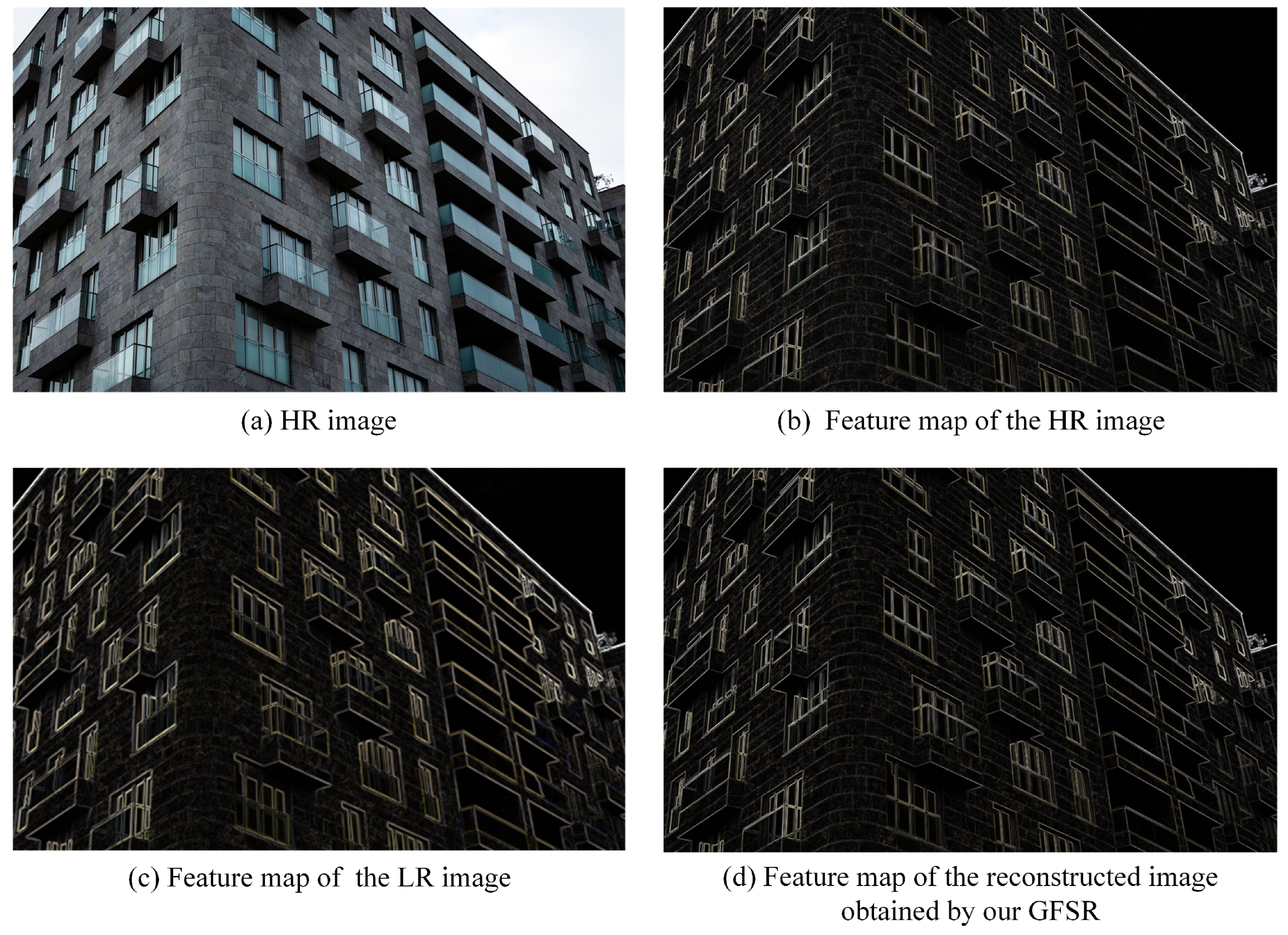
To verify the validity of the structure prior, we also visualize the output of the gradient branch, as shown in Figure 6. For a given original HR image (as shown in Figure 6a), the corresponding edge gradient map is sharp and clear (as shown in Figure 6b). However, when we observe the gradient map corresponding to the LR image (as shown in Figure 6c), it can be found that its edges are relatively rough. While, from the gradient map obtained by our GFSR (as shown in Figure 6d), we can see that the gradient branch effectively restores the structural information of the building, which is accurate and finer. This is because the gradient map is able to be used as a structure prior to provide rich structural information for the super-resolution process on the trunk branch, thereby effectively restoring more abundant and more accurate structure, edge and texture details.
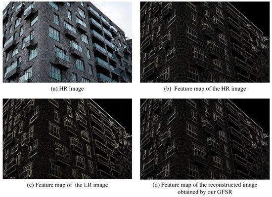
Figure 6.
Visualization of the feature map of Img_001 (Urban100).
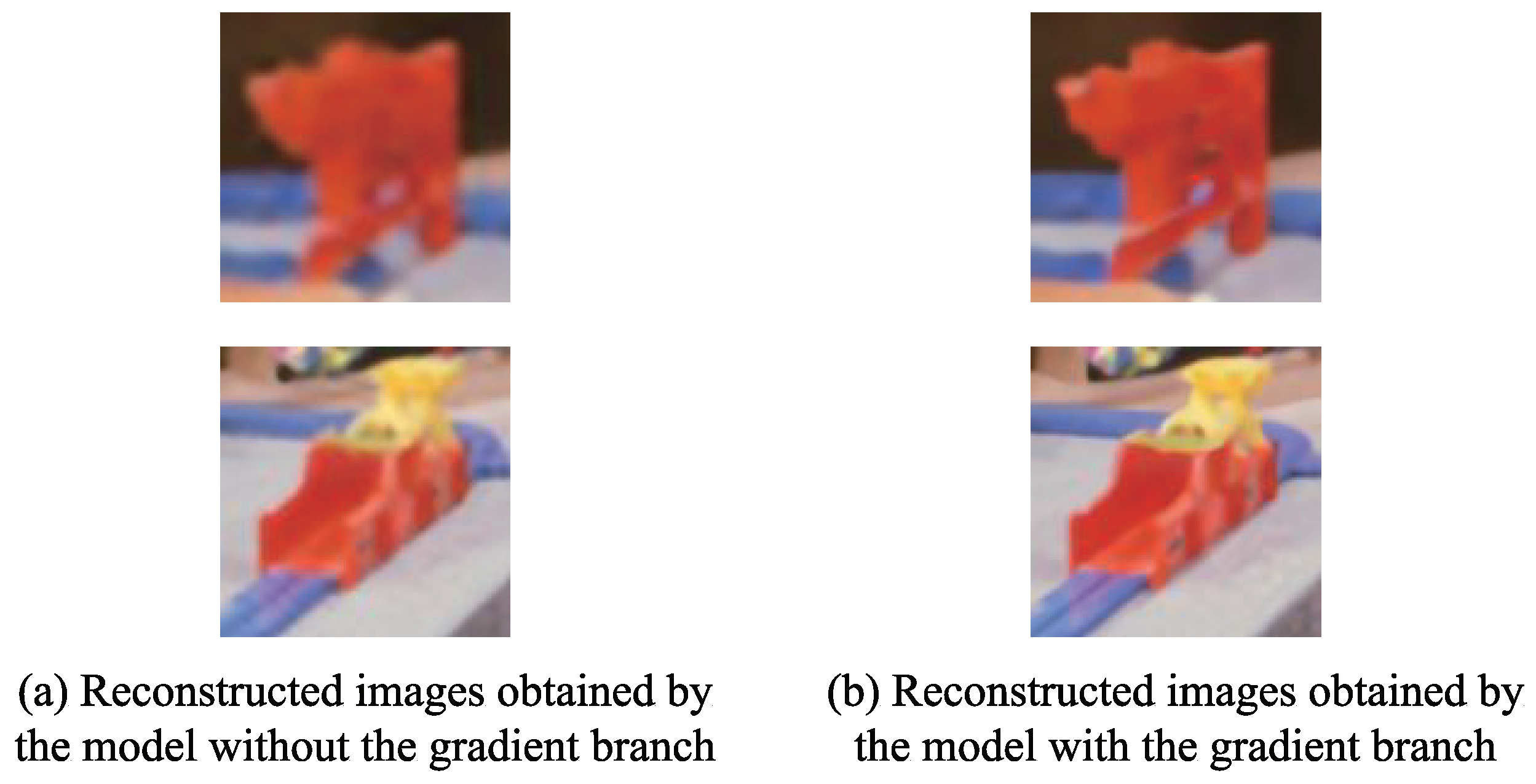
Figure 7 presents the comparison of the reconstructed images obtained by the models without or with the gradient branch. As can be seen from Figure 7, compared with the model without the gradient branch, the details of the reconstructed image obtained by the model with the gradient branch are closer to that of the reference image. Specifically, the edges and the textures around the toys are sharper and clearer in the reconstructed images obtained by the model with the gradient branch. In contrast, the corresponding edges and the textures are blurred in the reconstructed images obtained by the model without the gradient branch. Consequently, it can be seen that the gradient branch facilitates the model to reconstruct more abundant and accurate edge and texture details.
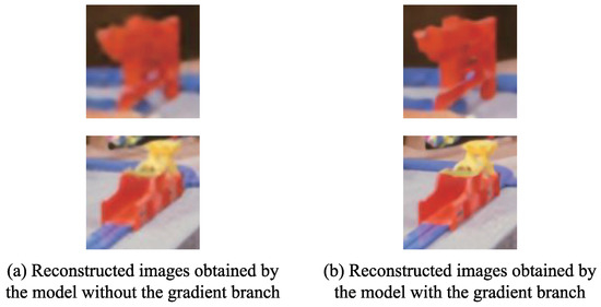
Figure 7.
Comparison of the reconstructed images obtained by different models.
4.3.3. Verification of the Effectiveness of Adaptive Weight Residual Unit
To verify the effectiveness of the proposed adaptive weight residual unit, we set the fixed weights for the residual structure refer to the EDSR model. Table 2 depicts the comparison of the best average PSNR metric of the models with different weights on the Set14 dataset in iterations. From Table 2, we can see that the model with the adaptive weight residual unit has achieved better super-resolution performance. This is mainly because the fixed weights lack flexibility in the training process, and the residual feature weights cannot be adjusted according to the specific network structure, so that the feature information extracted by the network cannot be fully exploited. While the adaptive weight residual unit we proposed is able to adaptively adjust the residual feature weights according to the different distributions of the features during training, so as to maximize the utilization of the extracted features.
Table 2.
Comparison of the average PSNR (dB) metric of the models corresponding to different weights on Set14 (×2) in iterations.
4.3.4. Verification of the Effectiveness of the Remaining Modules
To further verify the impact of the other three modules on the super-resolution performance, we conducted more experiments. We first treat the model using RIB and RRFB modules as a reference, namely the basic model, and then add each of the above-mentioned modules to the basic model respectively, and finally separately add the different above-mentioned modules to the basic model. Table 3 illustrates the best average PSNR of reconstructed images obtained by different models in iterations. As can be seen from Table 3, the GB module has the most obvious improvement in super-resolution performance if only the contribution of a single module is measured, and the model using all the modules simultaneously achieves consistently better outcomes compared to adding them independently. For the former, due to the GB module obtains the image structure information by extracting the gradient map, which effectively guides the super-resolution process. For the latter, due to the use of the ACAB, RFFB and GB modules increase the feature utilization, thereby reconstructing more image textures and details. Overall, these observations exhibit the superiority of our GFSR.
Table 3.
Effects of different modules. We report the best average PSNR(dB) on Set14 (×2) in iterations.
4.3.5. Selection of Related Hyperparameters
To verify the impact of different hyperparameters M and N on the model performance, we use 24 feature extraction modules including RRIB and RRRFB as the standard, then the number M of RRIB modules and the number N of RRRFB modules are set to different ratios (i.e., 1:1, 2:1, 3:1) to perform hyperparameter testing. Table 4 lists the best average PSNR and the amount of parameters obtained by different models. It can be seen from Table 4 that the model constructed according to the ratio of 2:1 (i.e., , ) achieves the best performance on the Set14 dataset in iterations.
Table 4.
Effects of different super-parameter of M and N. We report the best average PSNR(dB) on Set14 (×2) in iterations.
Then, we further conducted experiments on the selection of the number P of RRIB modules in the gradient branch. We compared the super-resolution performance of using 2, 3, 4, and 5 RRIB modules of the gradient branch, and Table 5 reports the best average PSNR obtained by different models on the Set14 dataset in iterations. As it can be seen in Table 5, with the increase of the number of RRIB modules, although the PSNR obtained by the model is continuously increasing, the amount of parameters of the model is also increasing simultaneously. When P is set to 5, the PSNR value obtained by the model is only slightly promoted, but the amount of parameters still has a significant increase. So, we choose as the hyper-parameter on the gradient branch.
Table 5.
Effects of different super-parameter of P. We report the best average PSNR(dB) on Set14 (×2) in iterations.
4.4. Comparison with State-of-the-Art Methods
To further test the adequacy of our proposed GFSR model, we compare it with seven CNN-based SR methods: SRCNN [30], VDSR [6], LapSRN [21], IDN [25], DPSR [22], IMDN [26], PAN [35], LAPAR-A [27], SMSR [28], DASR [24] and DeFiAN [23]. Inspired by [57], a self-ensemble strategy is introduced to further improve the proposed GFSR, and the improved model is named as GFSR+. The best average PSNR and SSIM of the reconstructed images obtained by the above SR methods using diverse scaling factors (×2, ×3, ×4) on the four standard datasets of Set5, Set14, BSD100 and Urban100 are listed in Table 6, where the optimal and suboptimal values marked in bold and underline, respectively.
Table 6.
Qualitative results of different SR models on the benchmark datasets.
It can be seen from Table 6 that both the best average PSNR and SSIM metrics of the reconstructed images obtained by the proposed GFSR+ are optimal for different scale factors on all datasets. Even for the proposed GFSR that does not incorporate the self-ensemble strategy, its best average PSNR and SSIM metrics of the reconstructed image are also optimal for different scale factors on all datasets compared to other state-of-the-art methods, which indicates that the proposed method achieves leading performance in terms of overall super-resolution performance.
To visually compare the reconstructed images obtained by different SR methods from subjective vision, Figure 8, Figure 9, Figure 10 and Figure 11 show the reconstruction results of different methods in the same region with a scaling factor of 4, and the corresponding original HR image is given as a reference. From Figure 8, Figure 9, Figure 10 and Figure 11, it can be seen that the vast majority of methods cannot precisely reconstruct edge and texture details, and even generate severe artifacts. Conversely, our GFSR can reconstruct a clearer image with richer edge and texture details.
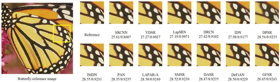
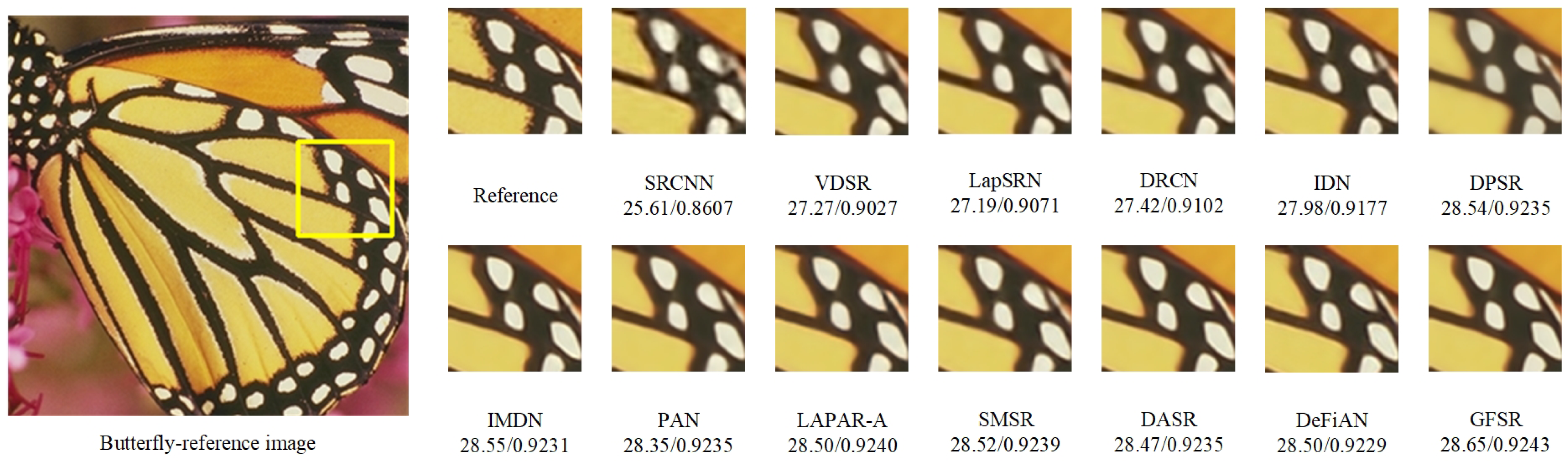
Figure 8.
Visual comparison of super-resolution results of ‘Butterfly’ (Set5) obtained by different SR algorithms with scaling factor ×4.
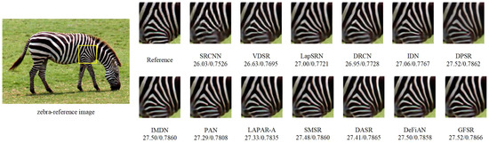
Figure 9.
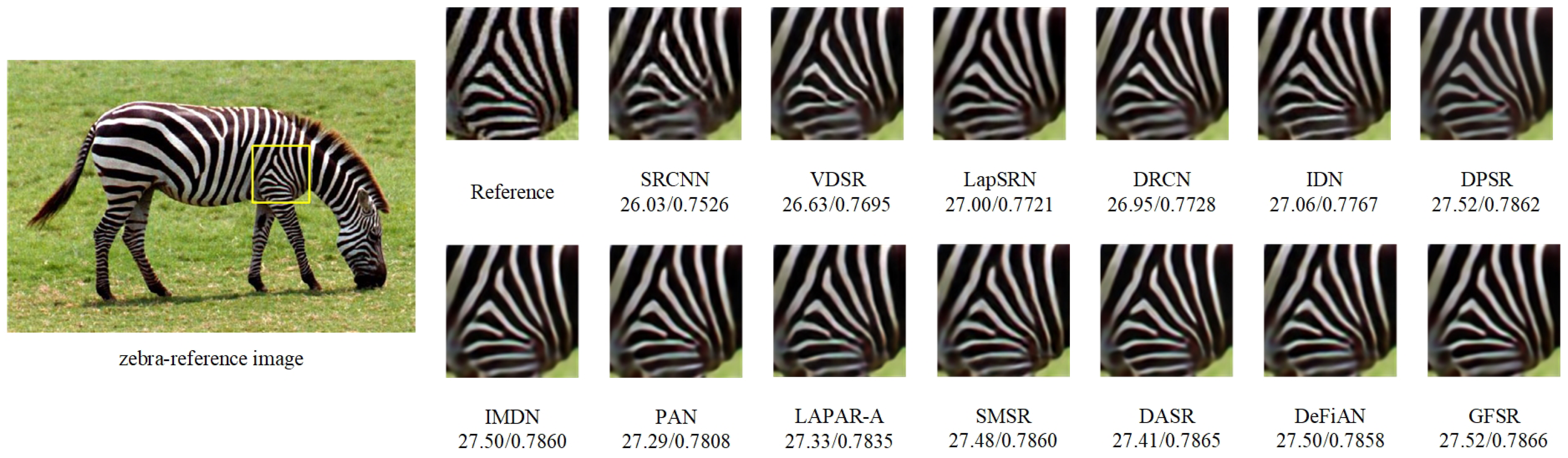
Visual comparison of super-resolution results of ‘Zebra’ (Set14) obtained by different SR algorithms with scaling factor ×4.
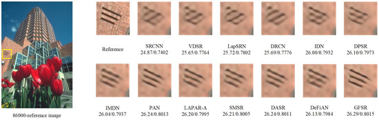
Figure 10.
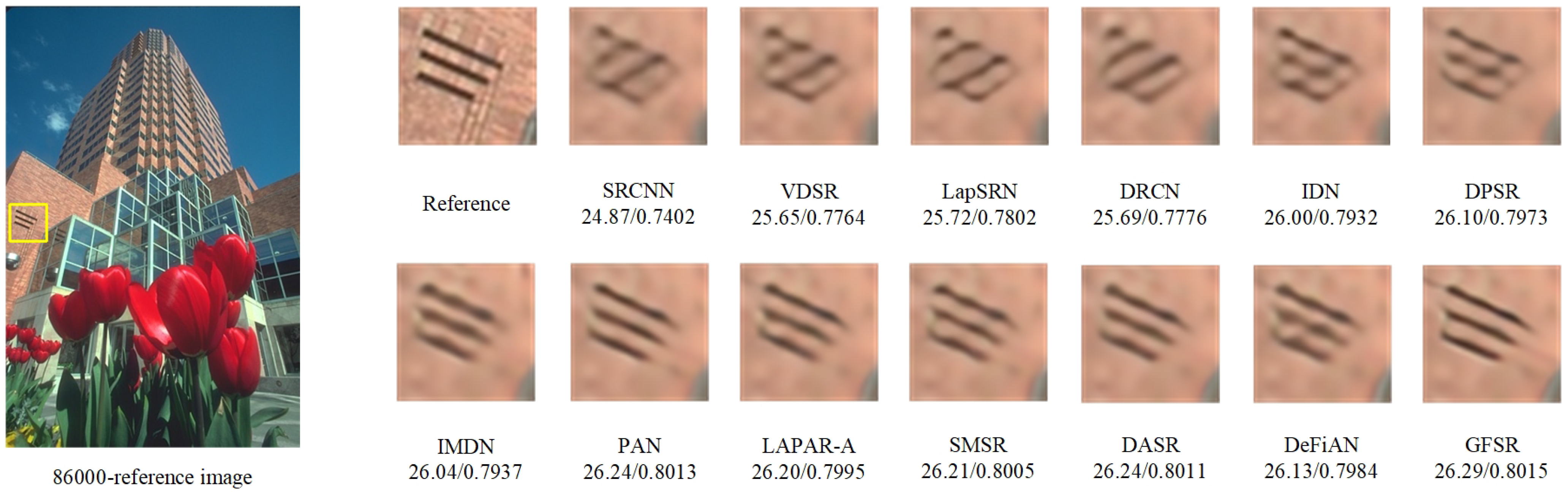
Visual comparison of super-resolution results of ‘86000’ (BSD100) obtained by different SR algorithms with scaling factor ×4.
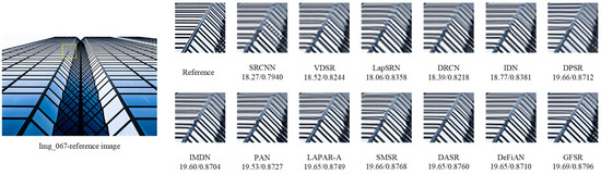
Figure 11.
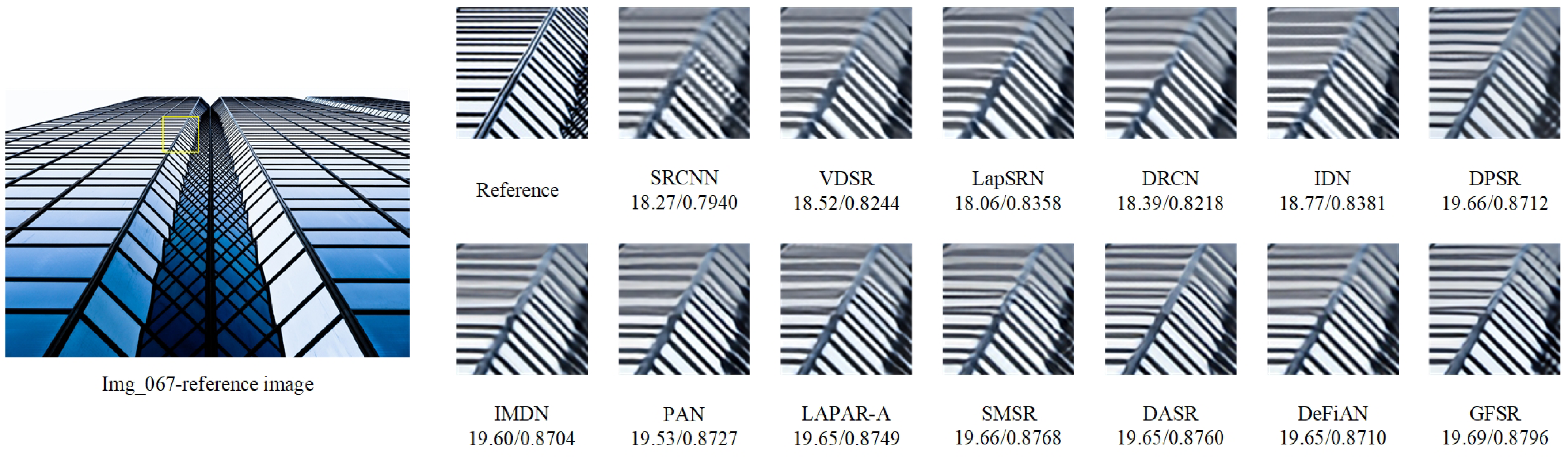
Visual comparison of super-resolution results of ‘Img_067’ (Urban100) obtained by different SR algorithms with scaling factor ×4.
Figure 8 illustrates the visual comparison of “Butterfly” images in the contrast methods in Set5. From Figure 8, we can see that the images reconstructed by SRCNN, VDSR, LapSRN, DRCN and DPSR are relatively blurry. Although IDN, LAPAP-A, SMSR and DeFiAN can recuperate more high-frequency information, the reconstructed images obtained also contain serious artifacts. Our proposed method, IMDN and DASR are able to recover richer detailed information and get better super-resolution results. Nonetheless, compared with IMDN and DASR, our GFSR method shows stronger performance in both contour preservation and detail restoration, which is reflected in a clearer overall contour, and more abundant information on the edges and textures of butterfly wings.
Figure 9 shows the visual comparison of the “Zebra” image in the contrast methods in Set14. It tends to be seen from Figure 9 that SRCNN, VDSR and DRCN cannot recover the edge and texture information effectively, and the generated image is blurry. Although LapSRN, IDN, DPSR, PAN, LAPAR-A, IMDN, DASR and DeFiAN can roughly recover edge and texture information, it also generates artifact detail. Our method can readily re-establish the stripes details of the zebra. This is mainly because our GFSR effectively integrates the extracted features of each layer, and utilizes the channel attention mechanism to explore the relationship between channel features.
Figure 10 presents the visual comparison of the “86000” image in the comparison method in BSD100. From Figure 10, it can be seen that although the reconstructed image of DeFiAN is superior to that of SRCNN, VDSR, LapSRN, DRCN, IDN and DPSR as far as edge details, there are a host number of artifacts. Contrasted with the DeFiAN, the methods such as IMDN, PAN, LAPAR-A, SMSR and DASR have fewer artifacts, and the reconstructed images obtained by them successfully smother the presence of artifacts, but edge recovery is inadequate compared with our proposed GFSR.
Figure 11 illustrates the visual comparison of the “Img_067” image in the comparison method in Urban100. As can be seen from Figure 11, a large portion of the methods, such as SRCNN, VDSR, LapSRN, DRCN and IDN, the reconstructed images appear severely blurred and even lose the fundamental structure. While DPSR, IMDN, PAN, LAPAR-A, SMSR, DASR and DeFiAN can recover the primary shapes, but cannot recover more image subtleties. Interestingly, our GFSR can get more clear outcomes and recover more high-frequency details. This is mainly because we use the prior guidance of gradient features in the model, which has a strong ability to reconstruct the edge features of buildings.
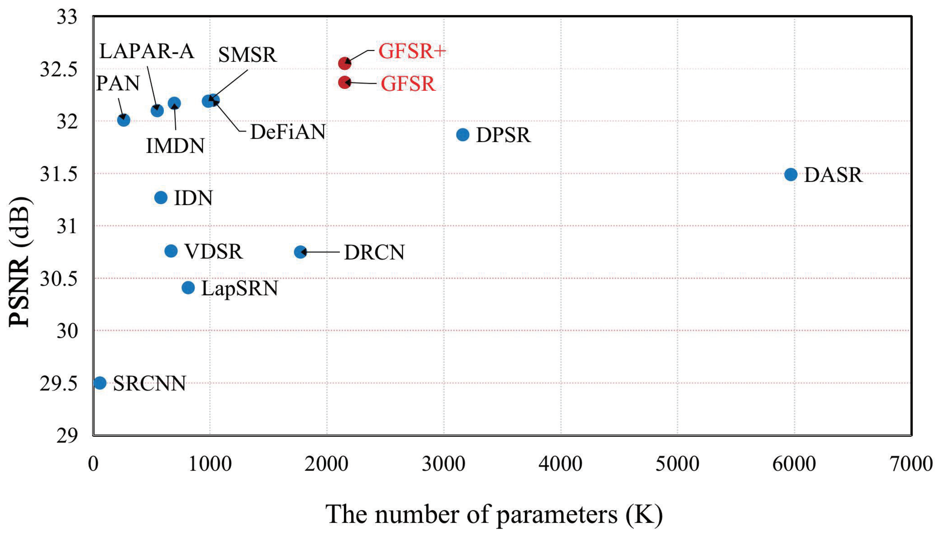
4.5. Analysis of the Number of Parameters of the Model
To visually measure the super-resolution performance and the number of parameters for different models, Figure 12 illustrates the comparison of different models in terms of the super-resolution performance and the number of parameters. It can be seen from Figure 12 that our GFSR and GFSR+ achieve a better trade-off between the super-resolution performance and the number of parameters compared to other methods. Specifically, compared with DASR, the proposed GFSR obtains a higher PSNR using only 36% of the parameters.

Figure 12.
Comparison of performance and number of parameters of different methods. Results are evaluated on Urban100 with scaling factor ×2.
5. Conclusions
To acquire beneficial structural prior to guide the super-resolution process effectively, a gradient-guided and multi-scale feature network for image super-resolution (GFSR) is proposed in this paper. Firstly, to fully utilize the image structure information, a novel network with a dual-branch structure is constructed, and the gradient feature map obtained from the gradient branch is employed as the structural prior of the high-frequency details. Secondly, two different multi-scale feature extraction modules are designed to acquire the luxuriant and effective features. Finally, the adaptive channel attention mechanism is incorporated into our GFSR model to highlight the significant channel features by adaptively exploring the dependence between channel features. Extensive experimental results demonstrate that the proposed GFSR achieves superior super-resolution results in comparison with state-of-the-art methods. However, the proposed GFSR model is slightly complex, we will focus on compressing the model while maintaining super-resolution performance to effectively promote computational efficiency in our future work.
Author Contributions
Conceptualization, J.C.; formal analysis, X.Z.; funding acquisition, D.H.; methodology, J.C. and X.Z.; software, F.C.; supervision, J.C. and D.H.; validation, J.C., X.Z. and F.C.; writing—original draft, J.C.; writing—review and editing, D.H. and X.Z. All authors have read and agreed to the published version of the manuscript.
Funding
This research was funded in part by the National Natural Science Foundation of China under Grant 61901183 and Grant 61976098, in part by the Fundamental Research Funds for the Central Universities Grant ZQN-921, in part by the Natural Science Foundation of Fujian Province under Grant 2019J01010561, in part by the Foundation of Fujian Education Department under Grant JAT170053, and in part by the Science and Technology Bureau of Quanzhou under Grant 2017G046.
Institutional Review Board Statement
Not applicable.
Informed Consent Statement
Not applicable.
Conflicts of Interest
The authors declare no conflict of interest.
References
- Zhou, Y.; Zhang, Y.; Xie, X.; Kung, S.Y. Image super-resolution based on dense convolutional auto-encoder blocks. Neurocomputing 2021, 423, 98–109. [Google Scholar] [CrossRef]
- Huang, Y.; Shao, L.; Frangi, A.F. Simultaneous Super-Resolution and Cross-Modality Synthesis of 3D Medical Images Using Weakly-Supervised Joint Convolutional Sparse Coding. In Proceedings of the 2017 IEEE Conference on Computer Vision and Pattern Recognition (CVPR), Honolulu, HI, USA, 21–26 July 2017; pp. 5787–5796. [Google Scholar] [CrossRef] [Green Version]
- Rasti, P.; Uiboupin, T.; Escalera, S.; Anbarjafari, G. Convolutional Neural Network Super Resolution for Face Recognition in Surveillance Monitoring. In Proceedings of the Articulated Motion and Deformable Objects, Palma de Mallorca, Spain, 13–15 July 2016; Springer International Publishing: Cham, Switzerland, 2016; pp. 175–184. [Google Scholar] [CrossRef]
- Mhatre, H.; Bhosale, V. Super resolution of astronomical objects using back propagation algorithm. In Proceedings of the 2016 International Conference on Inventive Computation Technologies (ICICT), Coimbatore, India, 26–27 August 2016; Volume 2, pp. 1–6. [Google Scholar] [CrossRef]
- Fu, Y.; Chen, J.; Zhang, T.; Lin, Y. Residual scale attention network for arbitrary scale image super-resolution. Neurocomputing 2021, 427, 201–211. [Google Scholar] [CrossRef]
- Kim, J.; Lee, J.K.; Lee, K.M. Accurate Image Super-Resolution Using Very Deep Convolutional Networks. In Proceedings of the 2016 IEEE Conference on Computer Vision and Pattern Recognition (CVPR), Las Vegas, NV, USA, 27–30 June 2016; pp. 1646–1654. [Google Scholar] [CrossRef] [Green Version]
- Ledig, C.; Theis, L.; Huszar, F.; Caballero, J.; Cunningham, A.; Acosta, A.; Aitken, A.; Tejani, A.; Totz, J.; Wang, Z.; et al. Photo-Realistic Single Image Super-Resolution Using a Generative Adversarial Network. In Proceedings of the 2017 IEEE Conference on Computer Vision and Pattern Recognition (CVPR), Honolulu, HI, USA, 21–26 July 2017; pp. 105–114. [Google Scholar] [CrossRef] [Green Version]
- Lim, B.; Son, S.; Kim, H.; Nah, S.; Lee, K.M. Enhanced Deep Residual Networks for Single Image Super-Resolution. In Proceedings of the 2017 IEEE Conference on Computer Vision and Pattern Recognition Workshops (CVPRW), Honolulu, HI, USA, 21–26 July 2017; pp. 1132–1140. [Google Scholar] [CrossRef] [Green Version]
- Kim, J.; Lee, J.K.; Lee, K.M. Deeply-Recursive Convolutional Network for Image Super-Resolution. In Proceedings of the 2016 IEEE Conference on Computer Vision and Pattern Recognition (CVPR), Las Vegas, NV, USA, 27–30 June 2016; pp. 1637–1645. [Google Scholar] [CrossRef] [Green Version]
- Ahn, N.; Kang, B.; Sohn, K.A. Fast, Accurate, and Lightweight Super-Resolution with Cascading Residual Network. In Proceedings of the Computer Vision—ECCV 2018, Munich, Germany, 8–14 September 2018; Springer International Publishing: Cham, Switzerland, 2018; pp. 256–272. [Google Scholar] [CrossRef] [Green Version]
- Tai, Y.; Yang, J.; Liu, X. Image Super-Resolution via Deep Recursive Residual Network. In Proceedings of the 2017 IEEE Conference on Computer Vision and Pattern Recognition (CVPR), Honolulu, HI, USA, 21–26 July 2017; pp. 2790–2798. [Google Scholar] [CrossRef]
- Li, J.; Fang, F.; Mei, K.; Zhang, G. Multi-scale Residual Network for Image Super-Resolution. In Proceedings of the Computer Vision—ECCV 2018, Munich, Germany, 8–14 September 2018; Springer International Publishing: Cham, Switzerland, 2018; pp. 527–542. [Google Scholar] [CrossRef]
- Zhang, Y.; Tian, Y.; Kong, Y.; Zhong, B.; Fu, Y. Residual Dense Network for Image Super-Resolution. In Proceedings of the 2018 IEEE/CVF Conference on Computer Vision and Pattern Recognition, Salt Lake City, UT, USA, 18–22 June 2018; pp. 2472–2481. [Google Scholar] [CrossRef] [Green Version]
- Liu, J.; Zhang, W.; Tang, Y.; Tang, J.; Wu, G. Residual Feature Aggregation Network for Image Super-Resolution. In Proceedings of the 2020 IEEE/CVF Conference on Computer Vision and Pattern Recognition (CVPR), Seattle, WA, USA, 14–19 June 2020; pp. 2356–2365. [Google Scholar] [CrossRef]
- Zhang, Y.; Li, K.; Li, K.; Wang, L.; Zhong, B.; Fu, Y. Image Super-Resolution Using Very Deep Residual Channel Attention Networks. In Proceedings of the Computer Vision—ECCV 2018, Munich, Germany, 8–14 September 2018; Springer International Publishing: Cham, Switzerland, 2018; pp. 294–310. [Google Scholar] [CrossRef] [Green Version]
- Ma, C.; Rao, Y.; Cheng, Y.; Chen, C.; Lu, J.; Zhou, J. Structure-Preserving Super Resolution with Gradient Guidance. In Proceedings of the 2020 IEEE/CVF Conference on Computer Vision and Pattern Recognition (CVPR), Seattle, WA, USA, 14–19 June 2020; pp. 7766–7775. [Google Scholar] [CrossRef]
- Shang, T.; Dai, Q.; Zhu, S.; Yang, T.; Guo, Y. Perceptual Extreme Super Resolution Network with Receptive Field Block. In Proceedings of the 2020 IEEE/CVF Conference on Computer Vision and Pattern Recognition Workshops (CVPRW), Seattle, WA, USA, 14–19 June 2020; pp. 1778–1787. [Google Scholar] [CrossRef]
- Wei, P.; Xie, Z.; Lu, H.; Zhan, Z.; Ye, Q.; Zuo, W.; Lin, L. Component Divide-and-Conquer for Real-World Image Super-Resolution. In Proceedings of the Computer Vision—ECCV 2020; Springer International Publishing: Cham, Switzerland, 2020; pp. 101–117. [Google Scholar] [CrossRef]
- Liu, S.; Huang, D.; Wang, Y. Receptive Field Block Net for Accurate and Fast Object Detection. In Proceedings of the Computer Vision—ECCV 2018, Munich, Germany, 8–14 September 2018; Springer International Publishing: Cham, Switzerland, 2018; pp. 404–419. [Google Scholar] [CrossRef] [Green Version]
- Wang, Q.; Wu, B.; Zhu, P.; Li, P.; Zuo, W.; Hu, Q. ECA-Net: Efficient Channel Attention for Deep Convolutional Neural Networks. In Proceedings of the 2020 IEEE/CVF Conference on Computer Vision and Pattern Recognition (CVPR), Seattle, WA, USA, 14–19 June 2020; pp. 11531–11539. [Google Scholar] [CrossRef]
- Lai, W.; Huang, J.; Ahuja, N.; Yang, M. Deep Laplacian Pyramid Networks for Fast and Accurate Super-Resolution. In Proceedings of the 2017 IEEE Conference on Computer Vision and Pattern Recognition (CVPR), Honolulu, HI, USA, 21–26 July 2017; pp. 5835–5843. [Google Scholar] [CrossRef] [Green Version]
- Zhang, K.; Zuo, W.; Zhang, L. Deep Plug-And-Play Super-Resolution for Arbitrary Blur Kernels. In Proceedings of the 2019 IEEE/CVF Conference on Computer Vision and Pattern Recognition (CVPR), Long Beach, CA, USA, 16–20 June 2019; pp. 1671–1681. [Google Scholar] [CrossRef] [Green Version]
- Huang, Y.; Li, J.; Gao, X.; Hu, Y.; Lu, W. Interpretable Detail-Fidelity Attention Network for Single Image Super-Resolution. IEEE Trans. Image Process. 2021, 30, 2325–2339. [Google Scholar] [CrossRef] [PubMed]
- Wang, L.; Wang, Y.; Dong, X.; Xu, Q.; Yang, J.; An, W.; Guo, Y. Unsupervised Degradation Representation Learning for Blind Super-Resolution. In Proceedings of the 2021 IEEE Conference on Computer Vision and Pattern Recognition (CVPR), Nashville, TN, USA, 19–25 June 2021; pp. 10576–10585. [Google Scholar] [CrossRef]
- Hui, Z.; Wang, X.; Gao, X. Fast and Accurate Single Image Super-Resolution via Information Distillation Network. In Proceedings of the 2018 IEEE/CVF Conference on Computer Vision and Pattern Recognition, Salt Lake City, UT, USA, 18–22 June 2018; pp. 723–731. [Google Scholar] [CrossRef] [Green Version]
- Hui, Z.; Gao, X.; Yang, Y.; Wang, X. Lightweight Image Super-Resolution with Information Multi-Distillation Network. In Proceedings of the 27th ACM International Conference on Multimedia—MM 2019, Nice, France, 21–25 October 2019; Association for Computing Machinery: New York, NY, USA, 2019; pp. 2024–2032. [Google Scholar] [CrossRef] [Green Version]
- Li, W.; Zhou, K.; Qi, L.; Jiang, N.; Lu, J.; Jia, J. LAPAR: Linearly-Assembled Pixel-Adaptive Regression Network for Single Image Super-resolution and Beyond. Adv. Neural Inf. Process. Syst. 2020, 33, 20343–20355. [Google Scholar]
- Wang, L.; Dong, X.; Wang, Y.; Ying, X.; Lin, Z.; An, W.; Guo, Y. Exploring Sparsity in Image Super-Resolution for Efficient Inference. In Proceedings of the 2021 IEEE Conference on Computer Vision and Pattern Recognition (CVPR), Nashville, TN, USA, 19–25 June 2021; pp. 4915–4924. [Google Scholar] [CrossRef]
- He, K.; Zhang, X.; Ren, S.; Sun, J. Deep Residual Learning for Image Recognition. In Proceedings of the 2016 IEEE Conference on Computer Vision and Pattern Recognition (CVPR), Las Vegas, NV, USA, 27–30 June 2016; pp. 770–778. [Google Scholar] [CrossRef] [Green Version]
- Dong, C.; Loy, C.C.; He, K.; Tang, X. Image Super-Resolution Using Deep Convolutional Networks. IEEE Trans. Pattern Anal. Mach. Intell. 2016, 38, 295–307. [Google Scholar] [CrossRef] [PubMed] [Green Version]
- Itti, L.; Koch, C.; Niebur, E. A model of saliency-based visual attention for rapid scene analysis. IEEE Trans. Pattern Anal. Mach. Intell. 1998, 20, 1254–1259. [Google Scholar] [CrossRef] [Green Version]
- Lu, Y.; Zhou, Y.; Jiang, Z.; Guo, X.; Yang, Z. Channel Attention and Multi-level Features Fusion for Single Image Super-Resolution. In Proceedings of the 2018 IEEE Visual Communications and Image Processing (VCIP), Taichung, Taiwan, 9–12 December 2018; pp. 1–4. [Google Scholar] [CrossRef] [Green Version]
- Dai, T.; Cai, J.; Zhang, Y.; Xia, S.; Zhang, L. Second-Order Attention Network for Single Image Super-Resolution. In Proceedings of the 2019 IEEE/CVF Conference on Computer Vision and Pattern Recognition (CVPR), Long Beach, CA, USA, 16–20 June 2019; pp. 11057–11066. [Google Scholar] [CrossRef]
- Niu, B.; Wen, W.; Ren, W.; Zhang, X.; Yang, L.; Wang, S.; Zhang, K.; Cao, X.; Shen, H. Single Image Super-Resolution via a Holistic Attention Network. In Proceedings of the Computer Vision—ECCV 2020, Glasgow, UK, 23–28 August 2020; Springer International Publishing: Cham, Switzerland, 2020; pp. 191–207. [Google Scholar] [CrossRef]
- Zhao, H.; Kong, X.; He, J.; Qiao, Y.; Dong, C. Efficient Image Super-Resolution Using Pixel Attention. In Proceedings of the Computer Vision—ECCV 2020 Workshops; Springer International Publishing: Cham, Switzerland, 2020; pp. 56–72. [Google Scholar] [CrossRef]
- Xie, J.; Feris, R.S.; Sun, M.T. Edge-Guided Single Depth Image Super Resolution. IEEE Trans. Image Process. 2016, 25, 428–438. [Google Scholar] [CrossRef] [PubMed]
- Sun, J.; Sun, J.; Xu, Z.; Shum, H.Y. Gradient Profile Prior and Its Applications in Image Super-Resolution and Enhancement. IEEE Trans. Image Process. 2011, 20, 1529–1542. [Google Scholar] [CrossRef] [PubMed]
- Yan, Q.; Xu, Y.; Yang, X.; Nguyen, T.Q. Single Image Superresolution Based on Gradient Profile Sharpness. IEEE Trans. Image Process. 2015, 24, 3187–3202. [Google Scholar] [CrossRef] [PubMed]
- Yang, W.; Feng, J.; Yang, J.; Zhao, F.; Liu, J.; Guo, Z.; Yan, S. Deep Edge Guided Recurrent Residual Learning for Image Super-Resolution. IEEE Trans. Image Process. 2017, 26, 5895–5907. [Google Scholar] [CrossRef] [PubMed] [Green Version]
- Jiang, K.; Wang, Z.; Yi, P.; Wang, G.; Lu, T.; Jiang, J. Edge-Enhanced GAN for Remote Sensing Image Superresolution. IEEE Trans. Geosci. Remote Sens. 2019, 57, 5799–5812. [Google Scholar] [CrossRef]
- Szegedy, C.; Liu, W.; Jia, Y.; Sermanet, P.; Reed, S.; Anguelov, D.; Erhan, D.; Vanhoucke, V.; Rabinovich, A. Going deeper with convolutions. In Proceedings of the 2015 IEEE Conference on Computer Vision and Pattern Recognition (CVPR), Boston, MA, USA, 7–12 June 2015; pp. 1–9. [Google Scholar] [CrossRef] [Green Version]
- Szegedy, C.; Vanhoucke, V.; Ioffe, S.; Shlens, J.; Wojna, Z. Rethinking the Inception Architecture for Computer Vision. In Proceedings of the 2016 IEEE Conference on Computer Vision and Pattern Recognition (CVPR), Las Vegas, NV, USA, 27–30 June 2016; pp. 2818–2826. [Google Scholar] [CrossRef] [Green Version]
- Ma, W.; Wu, Y.; Wang, Z.; Wang, G. MDCN: Multi-Scale, Deep Inception Convolutional Neural Networks for Efficient Object Detection. In Proceedings of the 2018 24th International Conference on Pattern Recognition (ICPR), Beijing, China, 20–24 August 2018; pp. 2510–2515. [Google Scholar] [CrossRef] [Green Version]
- Ding, X.; Guo, Y.; Ding, G.; Han, J. ACNet: Strengthening the Kernel Skeletons for Powerful CNN via Asymmetric Convolution Blocks. In Proceedings of the 2019 IEEE/CVF International Conference on Computer Vision (ICCV), Seoul, Korea, 27–28 October 2019; pp. 1911–1920. [Google Scholar] [CrossRef] [Green Version]
- Wandell, B.A.; Winawer, J. Computational neuroimaging and population receptive fields. Trends Cogn. Sci. 2015, 19, 349–357. [Google Scholar] [CrossRef] [PubMed] [Green Version]
- Tai, Y.; Yang, J.; Liu, X.; Xu, C. MemNet: A Persistent Memory Network for Image Restoration. In Proceedings of the 2017 IEEE International Conference on Computer Vision (ICCV), Venice, Italy, 22–29 October 2017; pp. 4549–4557. [Google Scholar] [CrossRef] [Green Version]
- Jung, H.; Lee, R.; Lee, S.H.; Hwang, W. Active weighted mapping-based residual convolutional neural network for image classification. Multimed. Tools Appl. 2021, 80, 33139–33153. [Google Scholar] [CrossRef]
- Hu, J.; Shen, L.; Albanie, S.; Sun, G.; Wu, E. Squeeze-and-Excitation Networks. IEEE Trans. Pattern Anal. Mach. Intell. 2020, 42, 2011–2023. [Google Scholar] [CrossRef] [PubMed] [Green Version]
- Agustsson, E.; Timofte, R. NTIRE 2017 Challenge on Single Image Super-Resolution: Dataset and Study. In Proceedings of the 2017 IEEE Conference on Computer Vision and Pattern Recognition Workshops (CVPRW), Honolulu, HI, USA, 21–26 July 2017; pp. 1122–1131. [Google Scholar] [CrossRef]
- Bevilacqua, M.; Roumy, A.; Guillemot, C.; Alberi Morel, M.L. Low-Complexity Single-Image Super-Resolution based on Nonnegative Neighbor Embedding. In Proceedings of the British Machine Vision Conference; BMVA Press: Guildford, UK, 2012; pp. 135.1–135.10. [Google Scholar] [CrossRef] [Green Version]
- Zeyde, R.; Elad, M.; Protter, M. On Single Image Scale-Up Using Sparse-Representations. In Proceedings of the Curves and Surfaces; Springer: Berlin/Heidelberg, Germany, 2012; pp. 711–730. [Google Scholar] [CrossRef]
- Martin, D.; Fowlkes, C.; Tal, D.; Malik, J. A database of human segmented natural images and its application to evaluating segmentation algorithms and measuring ecological statistics. In Proceedings of the Eighth IEEE International Conference on Computer Vision (ICCV 2001), Vancouver, BC, Canada, 7–14 July 2001; Volume 2, pp. 416–423. [Google Scholar] [CrossRef] [Green Version]
- Huang, J.; Singh, A.; Ahuja, N. Single image super-resolution from transformed self-exemplars. In Proceedings of the 2015 IEEE Conference on Computer Vision and Pattern Recognition (CVPR), Boston, MA, USA, 7–12 June 2015; pp. 5197–5206. [Google Scholar] [CrossRef]
- Wang, Y.; Li, J.; Lu, Y.; Fu, Y.; Jiang, Q. Image quality evaluation based on image weighted separating block peak signal to noise ratio. In Proceedings of the International Conference on Neural Networks and Signal Processing, Nanjing, China, 14–17 December 2003; Volume 2, pp. 994–997. [Google Scholar] [CrossRef]
- Wang, Z.; Bovik, A.C.; Sheikh, H.R.; Simoncelli, E.P. Image quality assessment: From error visibility to structural similarity. IEEE Trans. Image Process. 2004, 13, 600–612. [Google Scholar] [CrossRef] [PubMed] [Green Version]
- Kingma, D.P.; Ba, J. Adam: A Method for Stochastic Optimization. arXiv 2014, arXiv:1412.6980. [Google Scholar]
- Timofte, R.; Rothe, R.; Van Gool, L. Seven Ways to Improve Example-Based Single Image Super Resolution. In Proceedings of the 2016 IEEE Conference on Computer Vision and Pattern Recognition (CVPR), Las Vegas, NV, USA, 27–30 June 2016; pp. 1865–1873. [Google Scholar] [CrossRef] [Green Version]
- Ketkar, N.; Moolayil, J. Automatic Differentiation in Deep Learning. In Deep Learning with Python: Learn Best Practices of Deep Learning Models with PyTorch; Apress: Berkeley, CA, USA, 2021; pp. 133–145. [Google Scholar] [CrossRef]

Publisher’s Note: MDPI stays neutral with regard to jurisdictional claims in published maps and institutional affiliations. |
© 2022 by the authors. Licensee MDPI, Basel, Switzerland. This article is an open access article distributed under the terms and conditions of the Creative Commons Attribution (CC BY) license (https://creativecommons.org/licenses/by/4.0/).