Abstract
In order to investigate the effect of a baseline control system (BCS) on dynamic and fatigue characteristics of modern wind turbines, the simulation results of a 5-MW wind turbine subjected to wind loading without and with considering BCS (No. 1 and No. 2, respectively) were compared. The displacement and moment of tower and blades were compared, and the rainflow counting algorithm was used to analyze the fatigue load expressed in damage equivalent load (DEL). The results indicate that the mean and maximum values of structural dynamic responses in No. 2 have a great reduction with wind speed exceeding the rated speed comparing to No. 1; the 3P (3-times the frequency of rotor speed) of the wind turbine rotor speed will be close to the tower fore-aft (FA) natural frequency with the wind velocity around the cut-in speed in No. 2, which caused larger dynamic responses, number of load cycles, and DELs for the tower compared with No. 1; when wind velocity exceeds the rated wind speed, the BCS caused higher fluctuation of loads, increasing the related DELs. It is concluded that when analyzing the dynamic responses and designing wind turbine tower and blades, taking the BCS into account during analysis is significant.
1. Introduction
Wind energy has been firmly established as the mainstream choice for new power generation. By 2030, the global installed capacity of wind power will exceed 2000 GW [1]. The primary target for designing wind turbine is to maximize the power output. The rotor diameter and tower height of modern wind turbines exceed 200 and 100 m, respectively, which increases the flexibility and slenderness ratio of the structure. What is more, the cost of a rotor and tower exceeds 35% of the overall turbine costs for land-based wind projects [2]. With the increase of the size and rated power, the reasonable dynamic and fatigue analysis of support structure and blades subjected to wind loads become more and more important. For modern wind turbines, the power output is controlled by regulating the blade-pitch angle and rotor speed based on the baseline control system (BCS). The conclusion can be obtained according to the Blade Element Momentum (BEM) theory [3] that the blade-pitch angle and rotor speed directly affect the aerodynamic loads for wind turbines. So compared with the condition neglecting the BCS, the aerodynamic and fatigue loads of wind turbine will change when considering the BCS during the structural dynamic analysis. However, the previous researches seldom considered the BCS when studying the dynamic characteristics of wind turbines, and always assumed that the blade-pitch and rotor speed angle are constant. Therefore, it is very necessary to estimate the influence of the BCS on dynamic response and fatigue characteristics of modern wind turbines.
During the last two or three decades, a number of approaches have been investigated to simulate the dynamic characteristics of wind turbine subjected to external loads. Thirstrup [4] derived the local loads of inertia and presented a wind turbine model to simulate the dynamic characteristics. Naguleswaran [5] studied the aerodynamic characteristics of blades by simplifying blades to cantilever beams. For an elastic wind turbine blade, Baumgart [6] presented a mathematical model by combining finite elements and virtual work. Kiyomiya et al. [7] utilized an FEM model studying the dynamic characteristics of wind turbine under the excitation of earthquake and wind loads. Murtagh et al. [8] associated the coupling of the tower/nacelle with the blade motion and found that the blade–tower interaction could lead to the blade tip response increase. Kallesøe [9] developed a detailed model for a rotor blade including the effects of gravity, pitch, and rotor speeds. Chen et al. [10] studied the coupling of blade and tower with a dynamic FEM to obtain response characteristics of a wind turbine subjected to wind load more accurately. Li et al. [11] analyzed the dynamic response of a tower using the finite element method. To compute the non-linear aeroelasticity of wind turbine, Gebhardt and Roccia [12] presented an aeroelastic model. Guo et al. [13] developed an integrated finite element model of a 5-MW wind turbine and studied the impact and mechanism of the dynamic interaction with considering the mechanical energy distribution during dynamic response. Shkara et al. [14] considered the blade–tower aerodynamic coupling, he used CFD and coupled model to predict the aerodynamic loads acting on the tower due to the vortex shedding from the front blades. Feliciano et al. [15] developed and verified a generalized analytical model allowing to efficiently estimate wind turbine tower displacements under a variety of flow conditions. Hu et al. [16] studied the dynamic response of tall offshore monopile steel wind turbine towers under wind, wave, and current through experiment. Banerjee et al. [17] investigated the dynamic response of a 5-MW offshore wind turbine with monopile foundation subjected to wind and wave actions by modeling a tower as a multi-degree of freedom system.
It is worth noting that few researchers took the variation of blade-pitch angle or/and rotor speed into account when analyzing the dynamic response of wind turbine. Nezamolmolki and Shooshtari [18] studied the tower displacements of wind turbines with different design load cases including different sources of nonlinearities, but they did not consider that the blade-pitch angle and rotor speed will change along different wind speeds during normal operation with BCS working. Feyzollahzadeh et al. [19] used a method named analytical transfer matrix method (TMM) studied the dynamic response of wind turbine towers and the results were compared with FEM. However, the FEM cannot consider the effect of control system on support structure dynamic responses and they also ignored the control system. In a turbulent wind field, although Pim et al. [20] investigated the aerodynamic interaction of a rotating blade, the blade-pitch angle and rotor speed were still constant during one simulation in time domain. In fact, for modern wind turbines during normal operation, the blade-pitch angle and/or rotor speed are not always constant, which are regulated according to the BCS. Therefore, more reasonable results of wind-induced response can be obtained when the BCS is considered.
During the whole lifetime, the wind turbine tower and blades experiences fatigue loads caused by fluctuating wind conditions, which may cause damage failure. In most cases, wind turbine is in the state of running to obtain energy from atmosphere with the power control system working. Therefore, reasonable dynamic analysis of wind turbine structure subjected to wind loads is an important guarantee to calculate the fatigue loads during normal operation. Although many researchers have made numerous contributions to the fatigue study of wind turbines [21,22,23,24,25], there are about 32 blade failures and 14 tower failures each year in the world, and the number is increasing over time [26]. For the safety of wind turbine structure, the safety of blades made in composite is becoming more important. And the considerably larger blades used in modern wind turbines has also made the safety of wind turbine more significant. It must be proved that the designed structure of wind turbine subjected to expected fatigue load is safety during service life. Hence, investigating the dynamic responses of large-scale wind turbine tower and blades during power production with BCS working is very important.
Simulating the normal operation with BCS working is difficult for traditional FEM to investigate aeroelastic stability and structural dynamic responses of wind turbines. The computational procedures for wind turbine have increased in recent years. In the National Renewable Energy Laboratory (NREL), Jonkman and Buhl [27] proposed an aeroelastic code FAST to predict the coupled dynamic responses of a wind turbine, which was applied to study scientific problems [28,29,30]. The techniques of multi-body system dynamics and modal analysis were used in the structural model. Jonkman et al. [31] proposed the appropriate BCS for a 5-MW NREL wind turbine and the strategy of the BCS is always used in industry. As an open simulation platform, the dynamics responses of blades and tower with the BCS working can be obtained by adjusting the input files and modifying the program. As we all know that the BCS is an important part of a wind turbine and will affect the aerodynamic loads applied on the structure. What is more, fatigue analysis is based on the results of dynamic response. Studying the influence of the BCS on the dynamic and fatigue characteristics of modern wind turbines is significant, useful, and helpful for improving the design and manufacture of wind turbine support structures and blades.
For modern large-scale wind turbines, the blade-pitch angle and rotor speed will change with different wind speeds according to the power control system during normal operation. Considering the BCS when calculating the dynamic responses of the tower and blades subjected to wind loads can obtain reasonable results, but it was always ignored in traditional research by using FEM. According to the aforementioned introduction, in this paper, the influence of the BCS on dynamic and fatigue characteristics of modern wind turbines was researched by comparing the dynamic responses of tower and blades with and without considering the BCS with wind speed from cut-in to cut-out. Using FAST, a 5-MW wind turbine under different wind scenarios is analyzed. The fatigue load expressed in damage equivalent load (DEL) was analyzed by using the algorithm of rainflow counting. The simulation results of dynamic and fatigue for two cases were compared. The research results are helpful and useful for the design of large-scale wind turbines.
2. Basic Models and Theory
2.1. General Motion Equations
In FAST [27], a multi-body dynamics formulation is used to obtain the results. The users can give the blades and tower mode shapes as input in terms. Based on Kane’s dynamics [32], the equations of motion are derived and implemented. By Newton’s laws of motion, Kane’s equations of motion for a holonomic system with n DOFs can be stated as follows [33,34]:
The generalized active forces and generalized inertia forces can be expressed in Equations (2) and (3), respectively, for a set of rigid bodies characterized by reference frame and center of mass point :
where and are the active forces on the rigid body , respectively; is the acceleration; is the mass of particle ; is the time derivative of the angular momentum of rigid body about in the inertial frame ; is the partial linear velocity; and is the partial angular velocity.
The multi-body formulation for Equation (1) can be written in Equation (4) [27,34]:
where is the mass matrix; is the nonlinear forcing function; , and are the vectors of DOF displacements, velocities and accelerations, respectively; is the control inputs; is the wind inputs; and is time.
FAST numerically linearizes the aeroelastic equations of motion by perturbing (represented by a ∆) each of the system variables about their respective operating point (op) values [27]:
Substituting these expressions into the equations of motion and expanding as a Taylor series approximation results in the second-order linearized representation of the equations [27]:
where is the mass matrix; is the damping matrix; is the stiffness matrix; is the control input matrix; and is the wind input disturbance matrix. The “” notation is used to signify that the partial derivatives are computed at the operating point.
More details about the related structural modeling theory in FAST can be seen in [33]. The 5-MW wind turbine model published by NWTC (National Wind Technology Center) by Jonkman et al. [31] is intended to serve as a standard model for research of modern wind turbines. The structural properties are shown in Table 1. The structural dynamic characteristics of the model can be obtained by modifying the program according to the properties of wind turbine.

Table 1.
Properties of the 5-MW NREL wind turbine [28,29,31].
2.2. Blade Element Momentum Theory Model
In order to estimate the wind loads applied on the blades, BEM theory [3,35] is the widely used method. The BEM theory is also used in FAST to calculate the aerodynamic loads. The BEM theory uses both angular and axial momentum balances by coupling momentum theory and blade element theory to determine the resulting forces and the flow on the blade as shown in tabure 1.
We are interested in the aerodynamic forces normal to and tangential to the rotor plane. In Figure 1, the local flapwise and edgewise forces, and are shown as follows:
where is the flow angle (detailed in [3,35]), is the distance between hub and element, is the drag force, and is the lift force. The approach of measuring the aerodynamic loads on the blade is in [3].
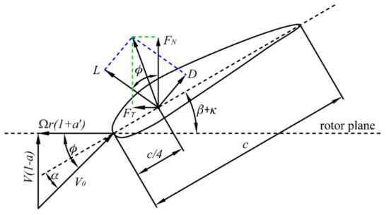
Figure 1.
Blade element forces and velocities in the BEM model [28,35].
2.3. Baseline Control System Model
For modern wind turbines, the BCS with a generator-torque controller and a blade-pitch controller is utilized to control the power output. Maximizing the power capture below the rated operation point and regulating generator speed above the rated operation point are the targets of generator-torque and blade-pitch controller, respectively.
2.3.1. Generator-Torque Controller
In the region of below-rated wind speed range, the generator torque must be varied as the square of the generator speed [36]:
and
where is the generator speed, is the generator torque, is the air density, is the gearbox ratio, is the rotor radius, is the maximum power coefficient, and is the optimum tip-speeds ratio (TSR).
2.3.2. Blade-Pitch Controller
In the region of above-rated wind speed range, the method of proportional-integral-derivative (PID) is used to control on the speed error between the rated generator speed and the generator speed. The related equation about the small perturbation of the blade-pitch angles about their operating point is shown as:
where is the small perturbation of angular velocity about the rated speed; , , and are the proportional, integral, and derivative gains, respectively.
During normal operation with the blade-pitch controller working, the blade-pitch angle can be adjusted by adding to the current blade-pitch angle to regulate the power output.
For the 5-MW NREL wind turbine used in this paper, we implemented the wind turbine’s BCS as an external dynamic link library (DLL) [31]. The source code for DLL can be found in the OpenFAST web site of NREL [37]. Based on the flowchart of the overall integrated control system calculations and the properties of the BCS [29,31], the executable program file can be obtained by using Visual Fortran Compiler [27], and then combined with the input file, the dynamic analysis of wind turbine under external load excitation can be realized. It should be pointed out that the gains for the PID control are 0.01882681 s, 0.008068634 and 0, respectively. More details about compiling source codes [37] and obtaining the appropriate gains of PID can be seen in [27,29,31].
3. Turbulent Wind Simulation and Fatigue Load Analysis Method
3.1. Turbulent Wind Simulation
It is very necessary for calculating the wind-induced response of tower and blades to simulate turbulent wind. Because of the statistical characteristic, the load simulation shall be performed based on the turbulent wind model. According to the IEC 61400-1 [38], the turbulence intensity and average wind speed at hub are used to generate the stochastic turbulence wind. Composing by the vertical-wind, across-wind and along-wind components, and the turbulent wind is a three-dimensional turbulent flow. The power characteristics of a turbulent wind field can be described by the power spectrum in related direction.
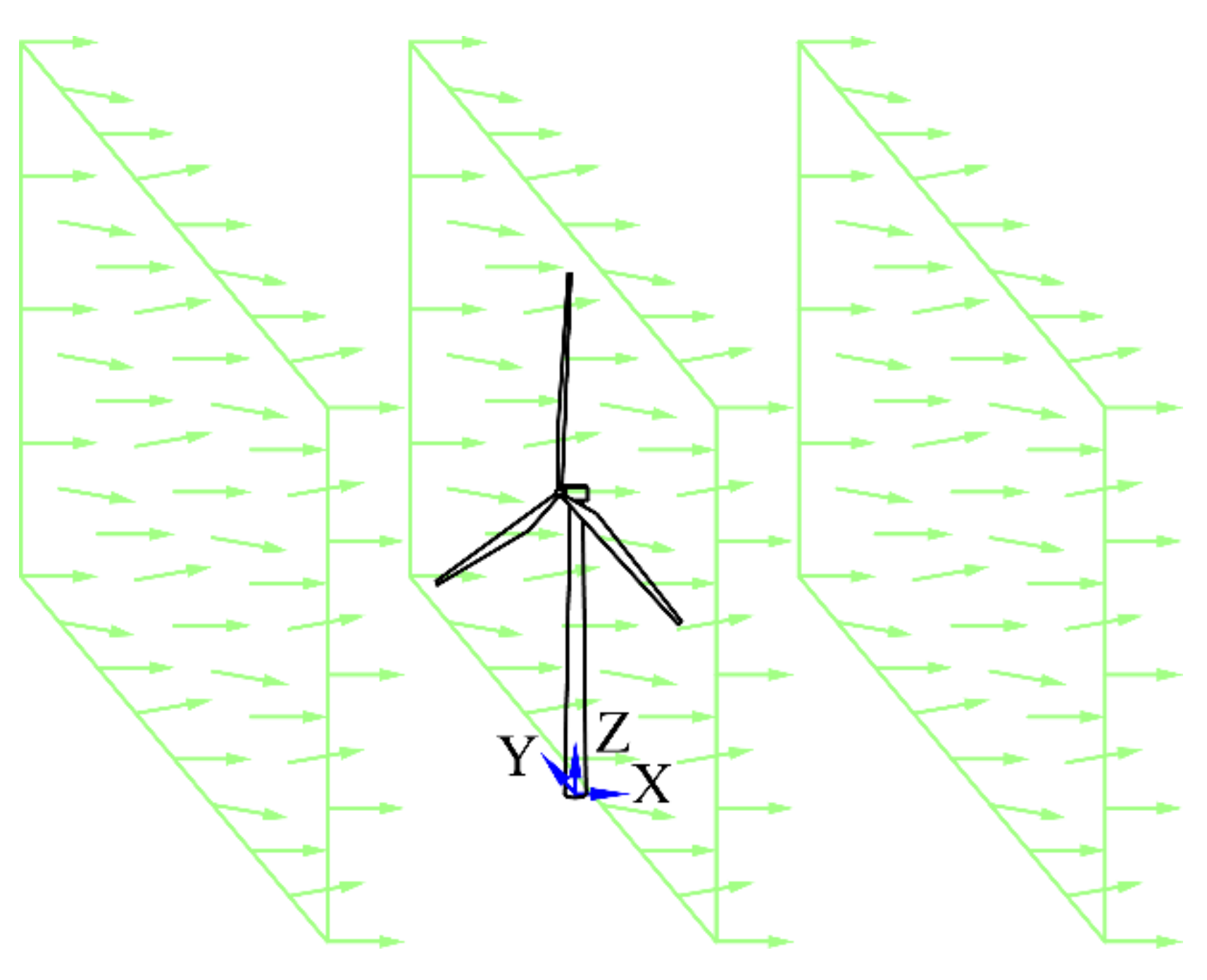
For the turbulence models, the vonKarman model is more suitable for wind tunnel turbulence, while the Kaimal model is suitable for atmospheric turbulence [39]. In this paper, during the simulation of turbulent wind, the turbulent model is the Kaimal spectra and the turbulence characteristic is Class A [38]. The relationship between the turbulence intensity and average wind speed at the hub (Vhub) is shown in Figure 2. To more accurately simulate the turbulent wind, we designed the width and height of the grid as 145 and 145 m respectively, and the height from the ground to the bottom of the grid is 17.5 m. A full-field, stochastic, turbulent wind is shown in Figure 3. Moreover, a set of 23 wind loads with different Vhub from 3 to 25 m/s are simulated by using the program TurbSim [40].
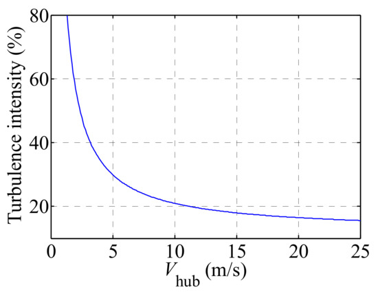
Figure 2.
Relationship between Vhub and turbulence intensity (Class A).
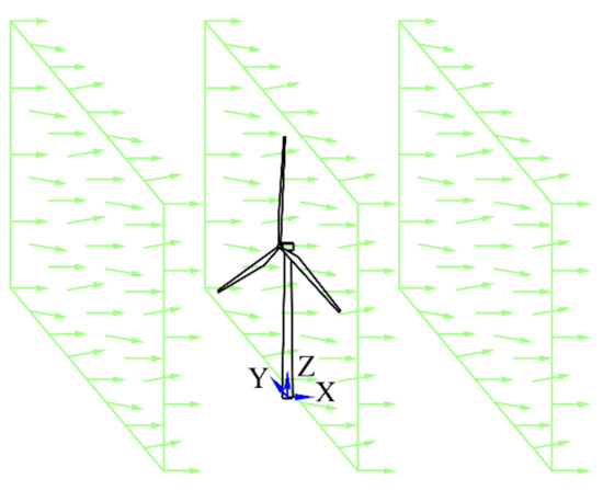
Figure 3.
The full-field turbulent wind.
3.2. Fatigue Load Analysis Method
The fatigue properties are very significant for the stability and security of the wind turbine tower and blades. Accurate fatigue analysis is advantageous for wind turbine structure design. Identifying individual load cycles becomes difficult when the loads occur more randomly. Because of matching experimental results well, the rainflow counting algorithm [41] was used to determine the related load amplitudes and the number of cycles. Based on Miner’s Rule [42], we assumed damage accumulates linearly with each of these cycles.
This study compares fatigue loads in the 5-MW NREL wind turbine between the two cases by using the program Mlife [43]. Thus, it is important to assess fatigue damage in terms of DELs. The equivalent amount of damage as original loads can be caused with constant-amplitude load ranges, and the technique was used by many researchers [44,45,46,47].
The relationship between cycles to failure and load amplitude given by the single relationship [48]:
where is the number of cycles at load level ; is a constant, and is a constant.
Based on Miner’s Rule, the damage , done by a number of load amplitudes , applied for cycles, respectively, can be obtained. The same fatigue damage supposes that DEL is done by a single load amplitude, , applied for cycles. Then:
So that:
where is the simulation time; is the DEL frequency.
In this paper, the DELs were calculated using a Wöhler exponent of 3 for the steel tower and 10 for the composite blades [45,48]. The value of is 1 and the related DEL is defined as the amplitude of the load that would have had to act on the component with a frequency of 1 Hz in order to cause the same damage as the acting load.
4. Numerical Results and Discussion
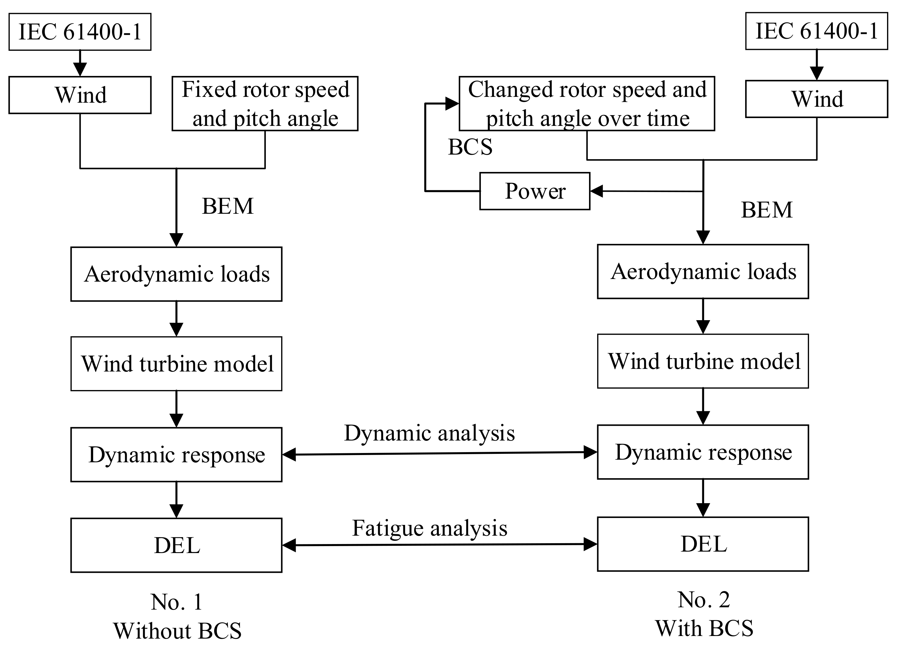
In No. 1, when the BCS is not considered, the fixed blade-pitch angle and rotor speed are 0 degree and 12.1 rpm, respectively. In No. 2, blade-pitch angle and rotor speed will be regulated according to the BCS. Figure 4 shows the flowchart of the two cases. It should be pointed out that in the two cases for each scenario, the wind speed time histories used as excitation loads are the same.
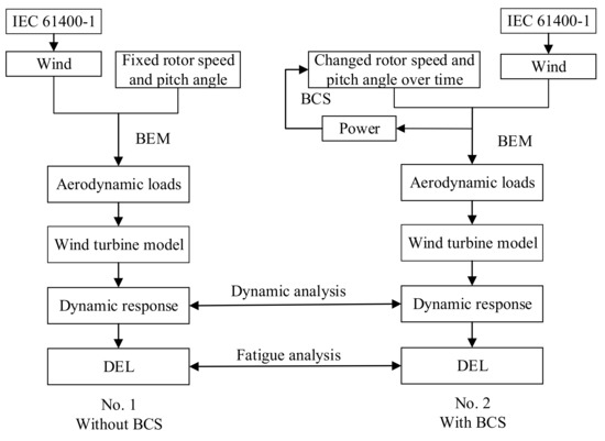
Figure 4.
Flowchart of the two cases.
4.1. Dynamic Analysis
Subjected to different wind scenarios with wind speed from cut-in to cut-out, the two cases are simulated. To analyze the influence of BCS on dynamic and fatigue characteristics of large-scale wind turbines, we chose two displacement components and four load components from the results of dynamic analysis to describe the wind turbine motions in major locations. The detailed descriptions about the six components are shown in Table 2.
Table 2.
Displacement and load components for wind turbine motions.
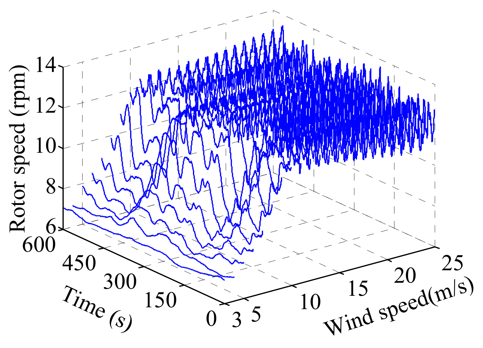
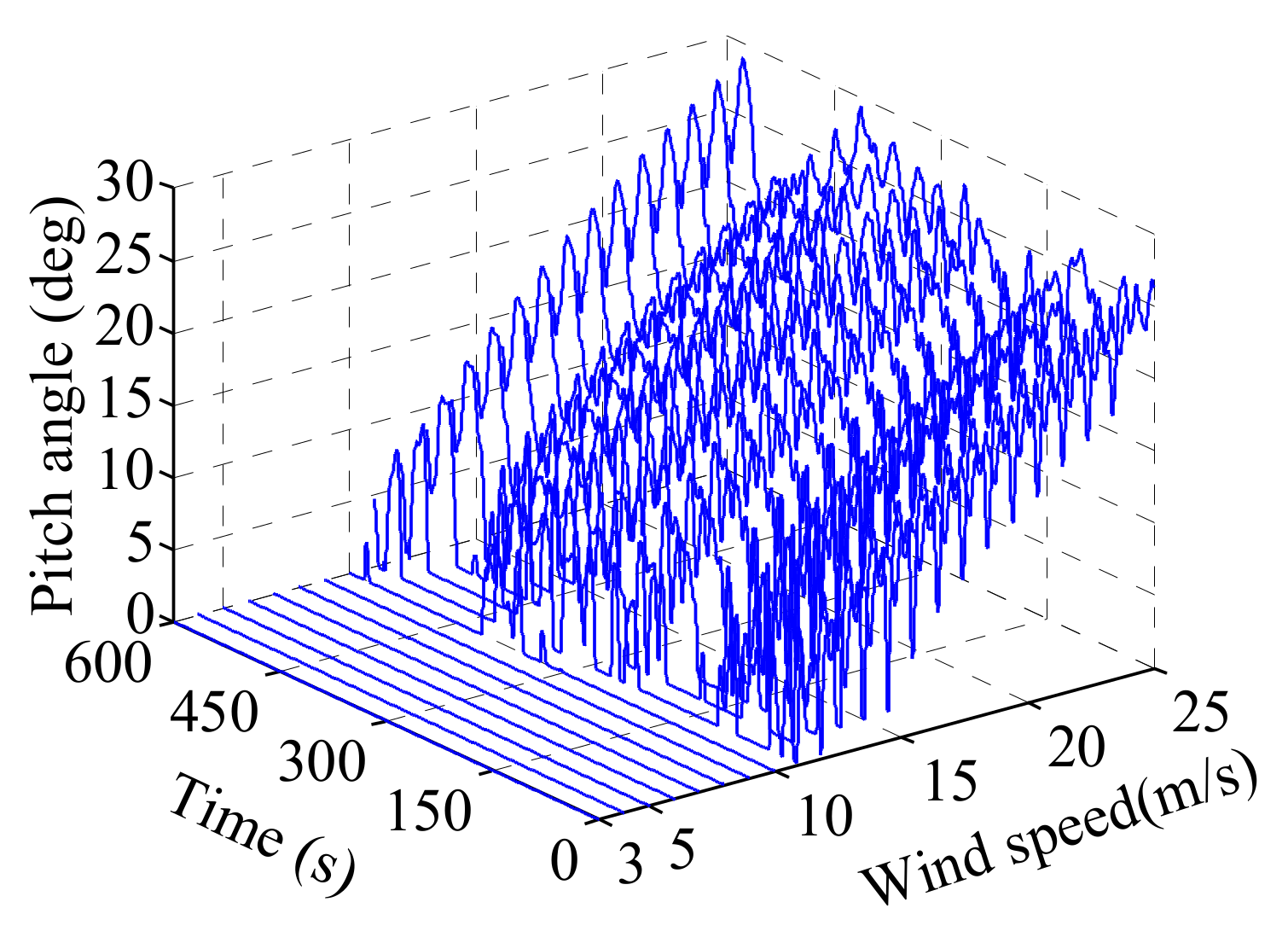
In No. 2, the three-dimensional curves graphical representation of the relationship between different average Vhub and rotor speed time histories is shown in Figure 5. And the related three-dimensional curves graphical for is shown in Figure 6. It is noted that when the wind speed is lower than the rated wind speed, the rotor speed increases with the increase of wind speed in the region of below-rated wind speed range; however, the rotor speed changes around the rated rotor speed in the region of above-rated wind speed range. It is also noted that the is zero in the region of below-rated wind speed range, and the increases with the increase of wind speed in the region of above-rated wind speed range. These are the results of BCS regulation.

Figure 5.
Rotor speed for different wind conditions with the BCS working.

Figure 6.
Blade-pitch angle for different wind conditions with the BCS working.
4.1.1. Effect of BCS on Mean Values of Dynamic Response
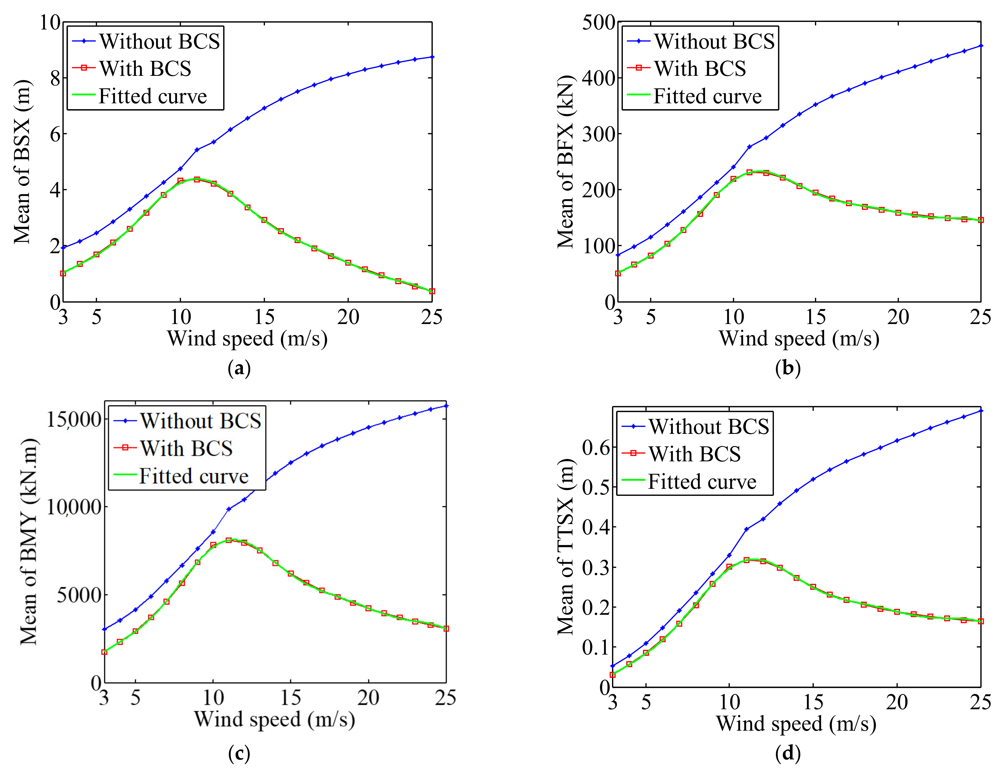
The mean values of the six components in ten minutes with different wind speeds in both cases and the fitted curves for No. 2 are shown in Figure 7. It can be seen that each mean value in No. 1 is larger than that in No. 2 with the same wind condition. It also can be seen that the six components in No. 1 have the same trend, the mean values increase with the increase of wind speed. The reason for this phenomenon is that in No. 1, the aerodynamic loads are large when the wind speed is high. However, in No. 2, the mean values increase first in the region of below-rated wind speed range and then decrease in the region of above-rated wind speed range. The reason is that the begins to increase when wind speed exceeds the rated wind speed (Figure 6) so that appropriate aerodynamic loads are obtained to make sure there is a constant level of torque. Table 3 shows the mean values of the six components in cut-in, rated, and cut-out wind speed and the difference between the two cases. From the table we can know that there are mean values reductions of more than 68% in the cut-out wind speed when the BCS working compared to the No. 1. The three series sine function fits are carried out and are shown in Equations (17)–(22) to describe the relationship between the mean values and the wind speeds when the BCS is working. It was obtained that the BCS has a great effect on the mean values of modern wind turbine structural dynamic responses.
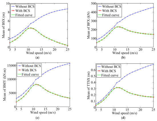
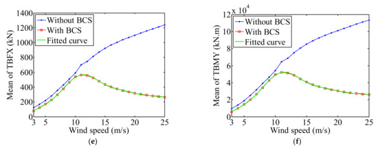
Figure 7.
Comparison of the mean values with respect to different mean wind levels between the two cases and the fitted curves for No. 2: (a) BSX, (b) BFX, (c) BMY, (d) TTSX, (e) TBFX, and (f) TBMY.
Table 3.
Mean values and difference between the two cases in cut-in, rated, and cut-out wind speed.
4.1.2. Effect of the BCS on Maximum Values of Dynamic Response
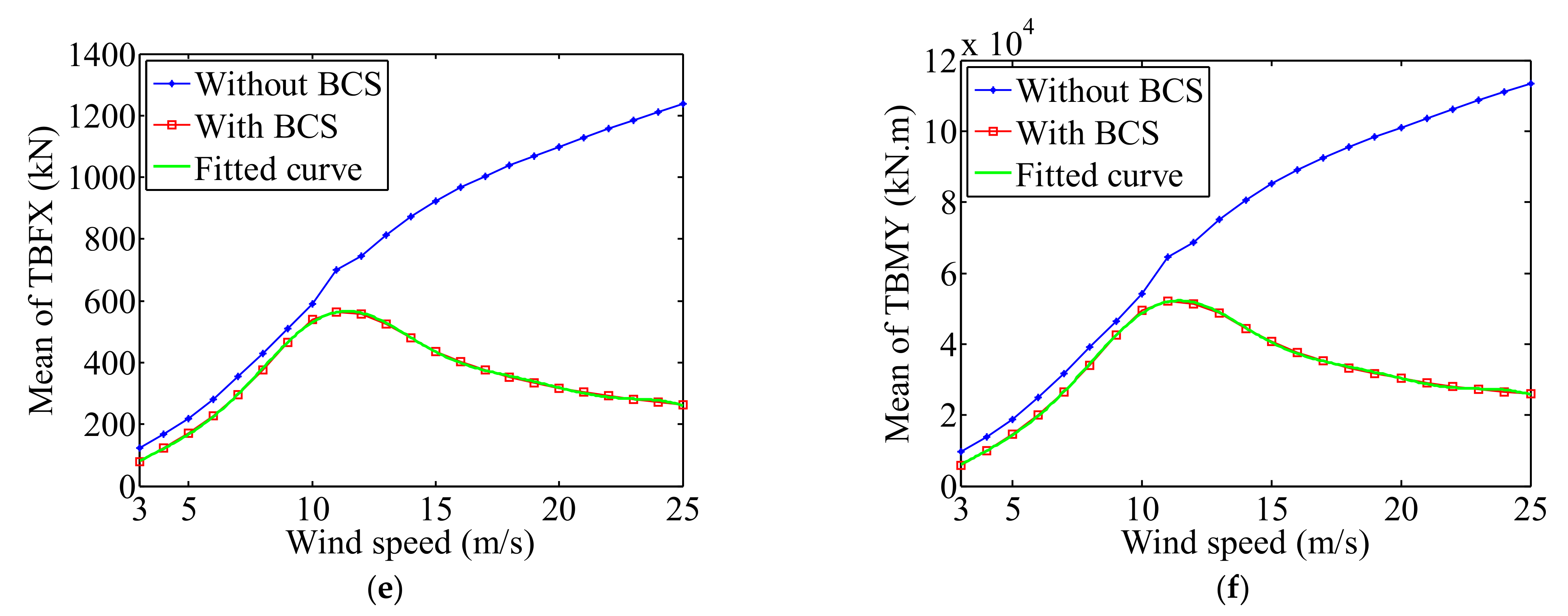
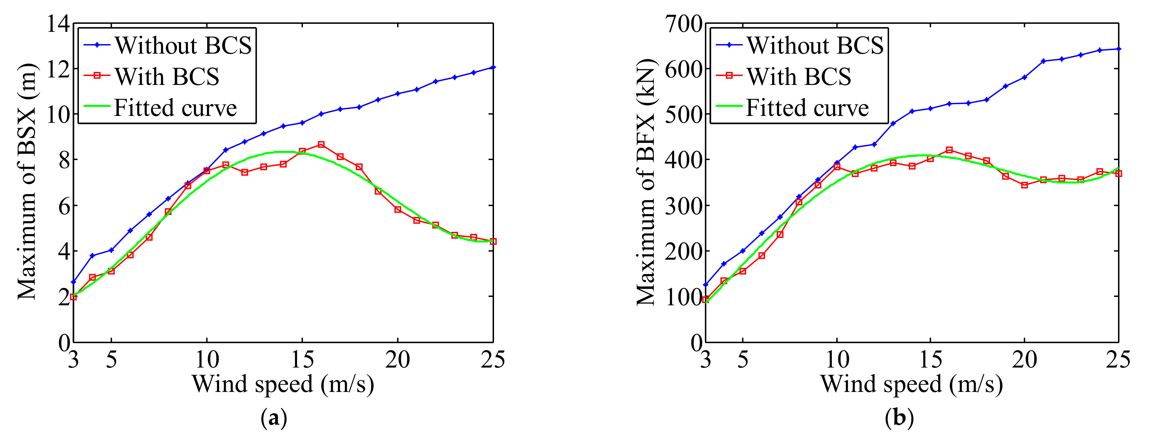
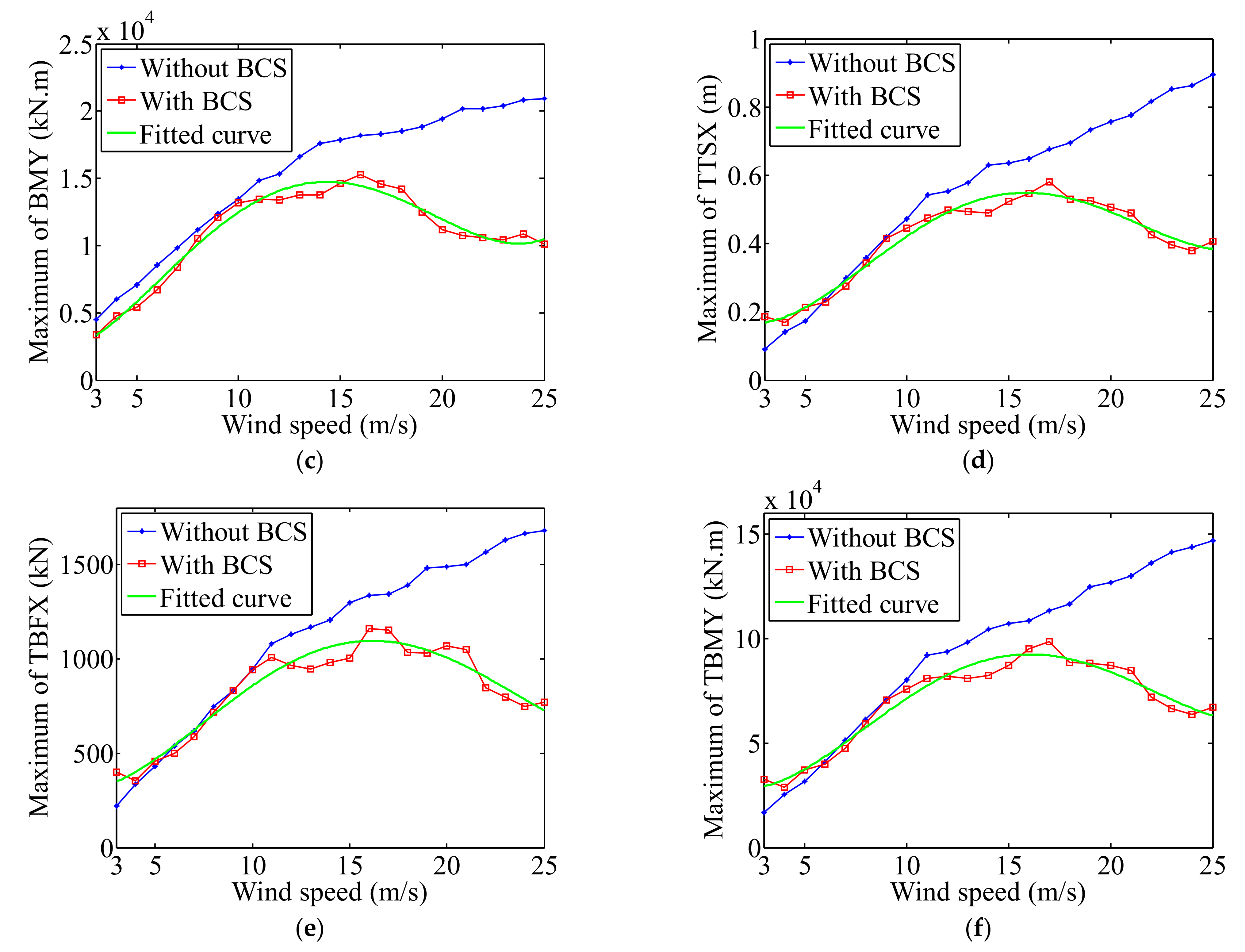
Figure 8 shows the maximum values of the six components from the 23 wind speeds between the two cases and the fitted curves for No. 2. We also found that the maximum values in No. 1 are always larger than those in No. 2 with the same wind condition. The fixed and rotor speed in No. 1 lead to the aerodynamic loads increase as wind speed, which causes the same trend for maximum results with the mean values. Because of the action of BCS, the maximum values in No. 2 increase first and then decrease with the increase of wind speed. The maximum values of the six parameters in cut-in, rated, and cut-out wind speed and Table 4 shows the difference between the two cases. It is observed that the BCS in No. 2 achieves reduction of maximum values by more than 42% in the cut-out wind speed compared to No. 1. The six fourth order polynomial fits are used to calculate the corresponding maximum values with respect to different wind speeds and they are shown in Equations (23)–(28).
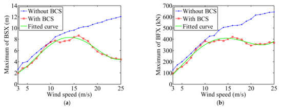
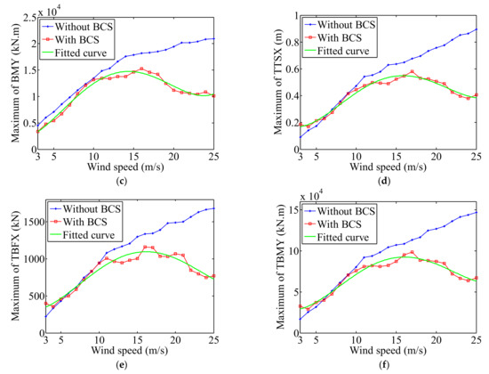
Figure 8.
Comparison of the maximum values with respect to different mean wind levels between the two cases and the fitted curves for No. 2: (a) BSX, (b) BFX, (c) BMY, (d) TTSX, (e) TBFX, and (f) TBMY.
Table 4.
Maximum values and difference between the two cases in cut-in, rated, and cut-out wind speed.
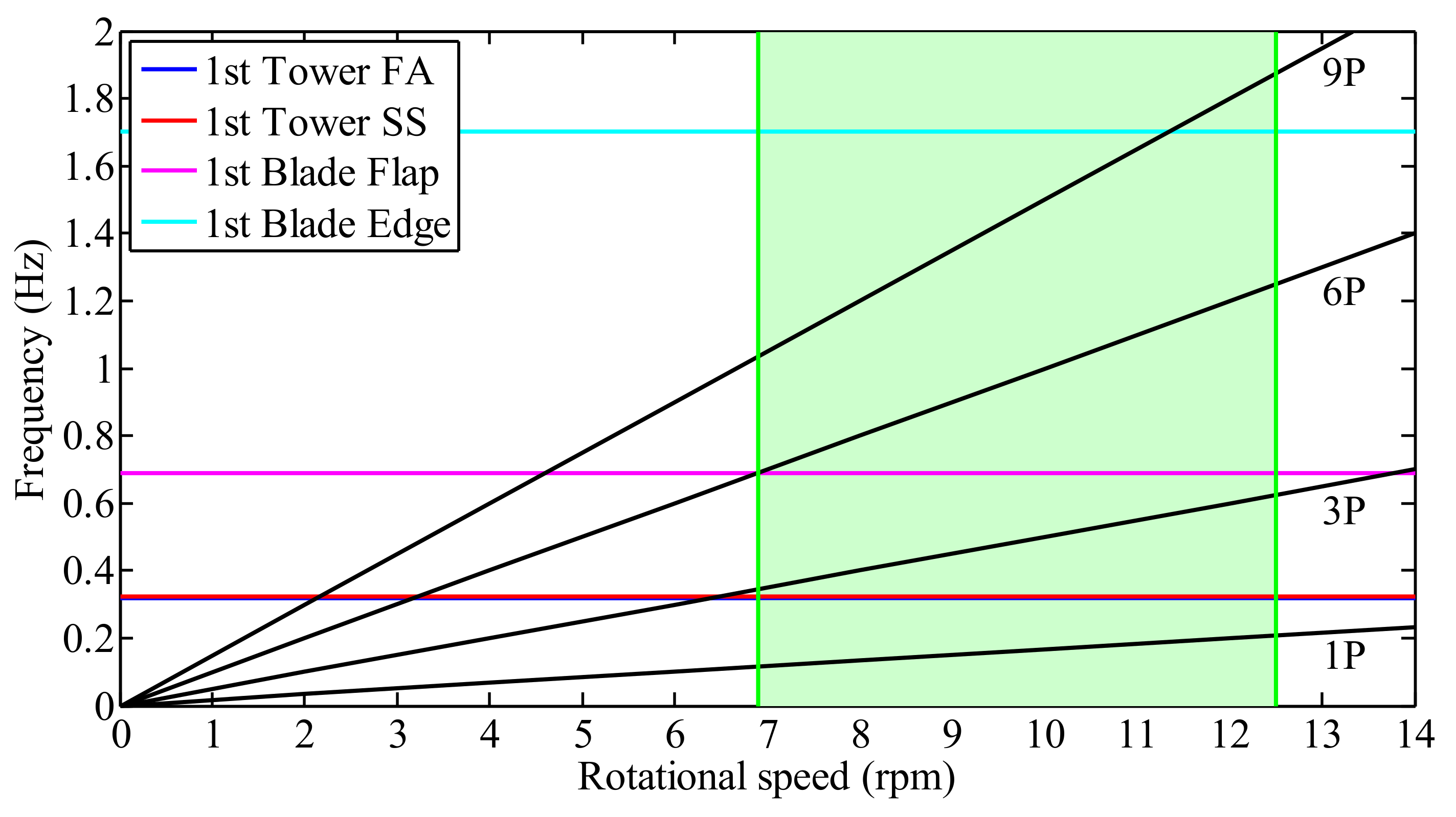
From the Figure 8 and Table 4, it is can be seen that the maximum values of the displacement and load components in tower with the wind speed around cut-in speed in No. 1 are smaller than that in No. 2. To find the reason of this phenomenon, the Campbell diagram of the wind turbine was calculated and shown in Figure 9. And the green shaded zone indicates the normal operating design range of the rotor speed. It should be noted that the Campbell diagram of a rotating machine consists of a plot of the natural frequencies of the system as functions of the spin speed on which the frequencies of the forcing excitation functions are superimposed, and is one of the most important tools for understanding the dynamic behavior of the rotating machine [49]. For the wind turbine with three blades, the first side-to-side and fore-aft tower frequencies are designed between the 1P (the frequency of rotor speed) and 3P during the total operational range in the Campbell diagram avoid the risk of resonance related to rotor speed harmonics [31,50,51,52]. In Figure 9, we find that in No. 2 the rotor speeds are around 7 rpm around the cut-in wind speed, which causes resonance with the 3P of the rotor speed closing to the first tower FA natural frequency. This is the reason of the phenomenon. It is also concluded that the BCS has a great effect on the maximum values of modern wind turbine structural dynamic responses.
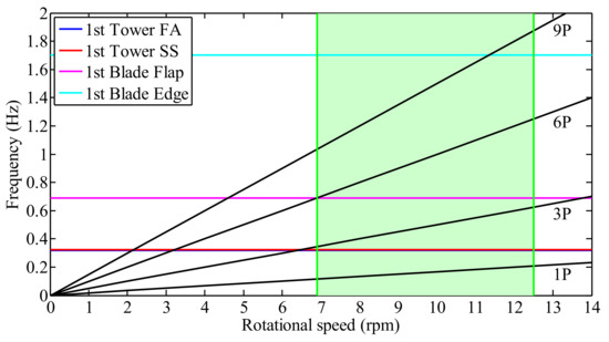
Figure 9.
Campbell diagram of the 5-MW wind turbine.
4.2. Fatigue Analysis
To study the fatigue property of wind turbines with the two cases, the results of fatigue analysis are expressed in DEL in major locations, BFX, BMY, TBFX, and TBMY. Before analyzing the DELs, we analyzed the rainflow cycles first.
4.2.1. Effect of BCS on Number of Rainflow Cycles
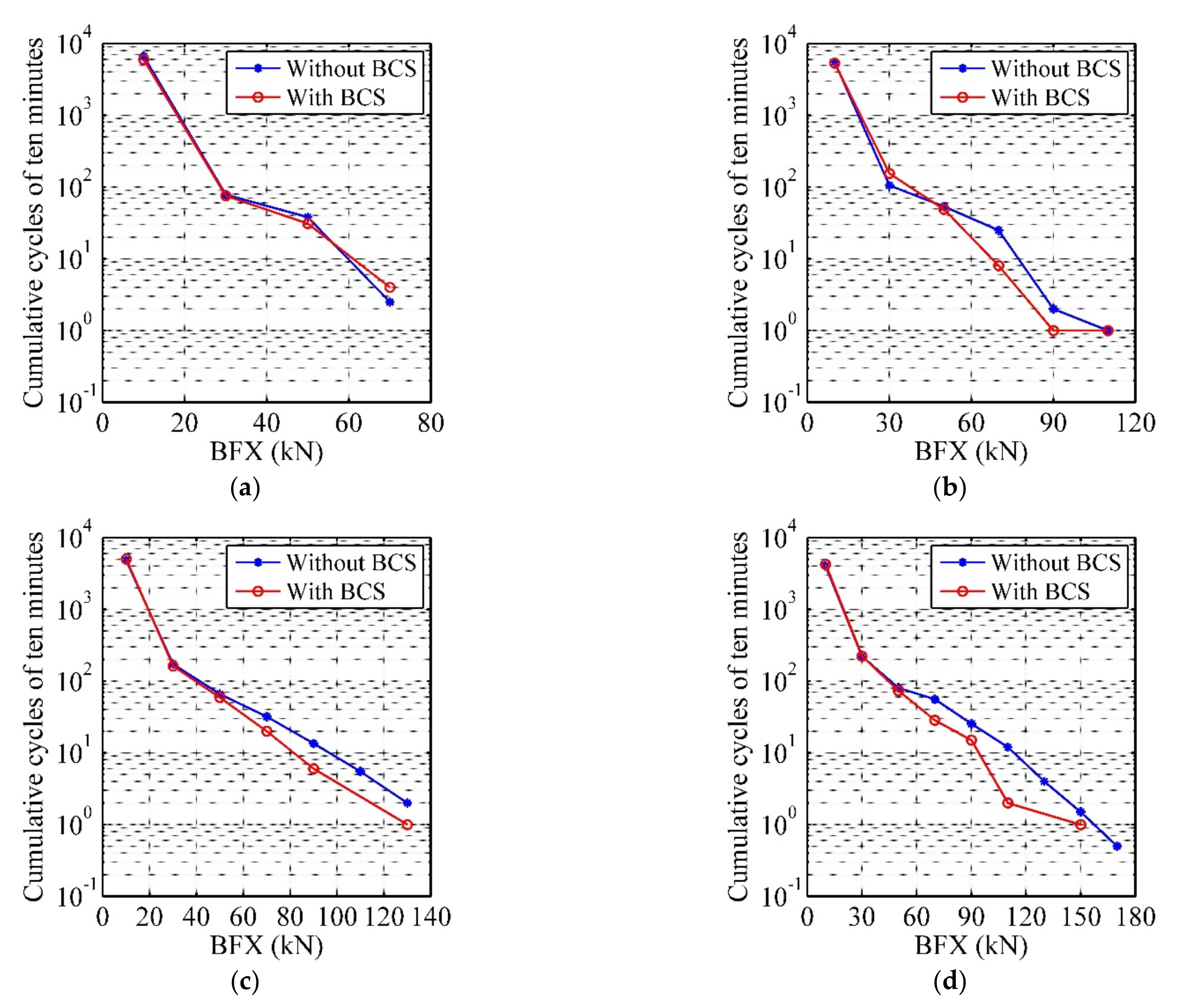
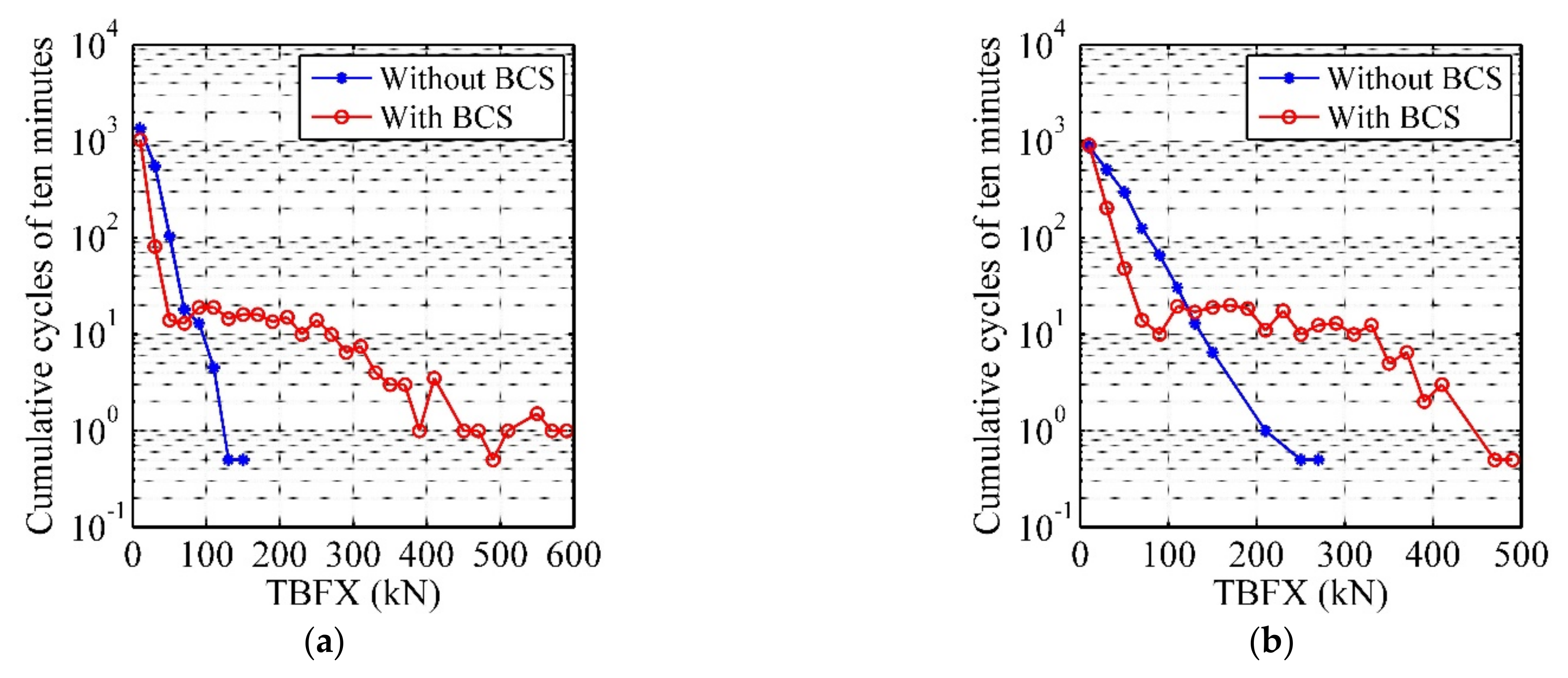
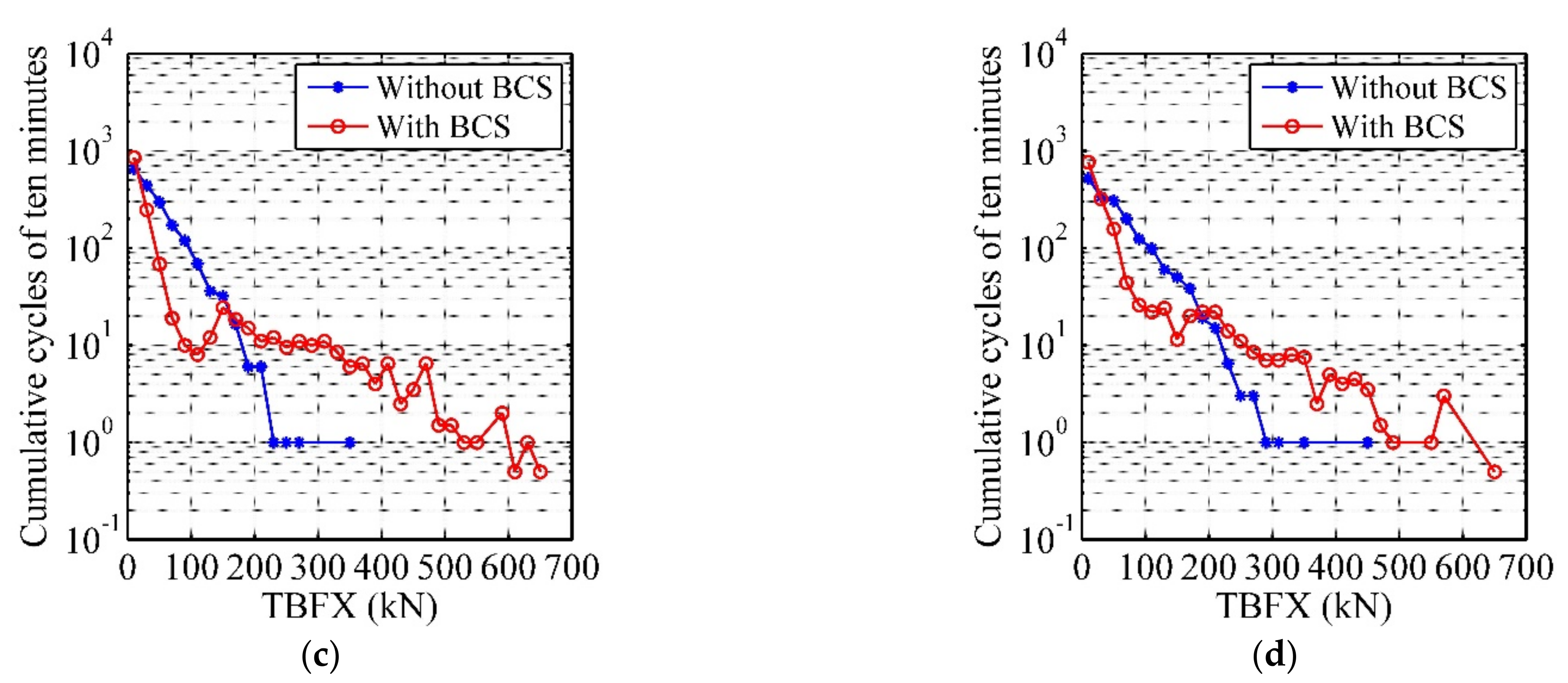
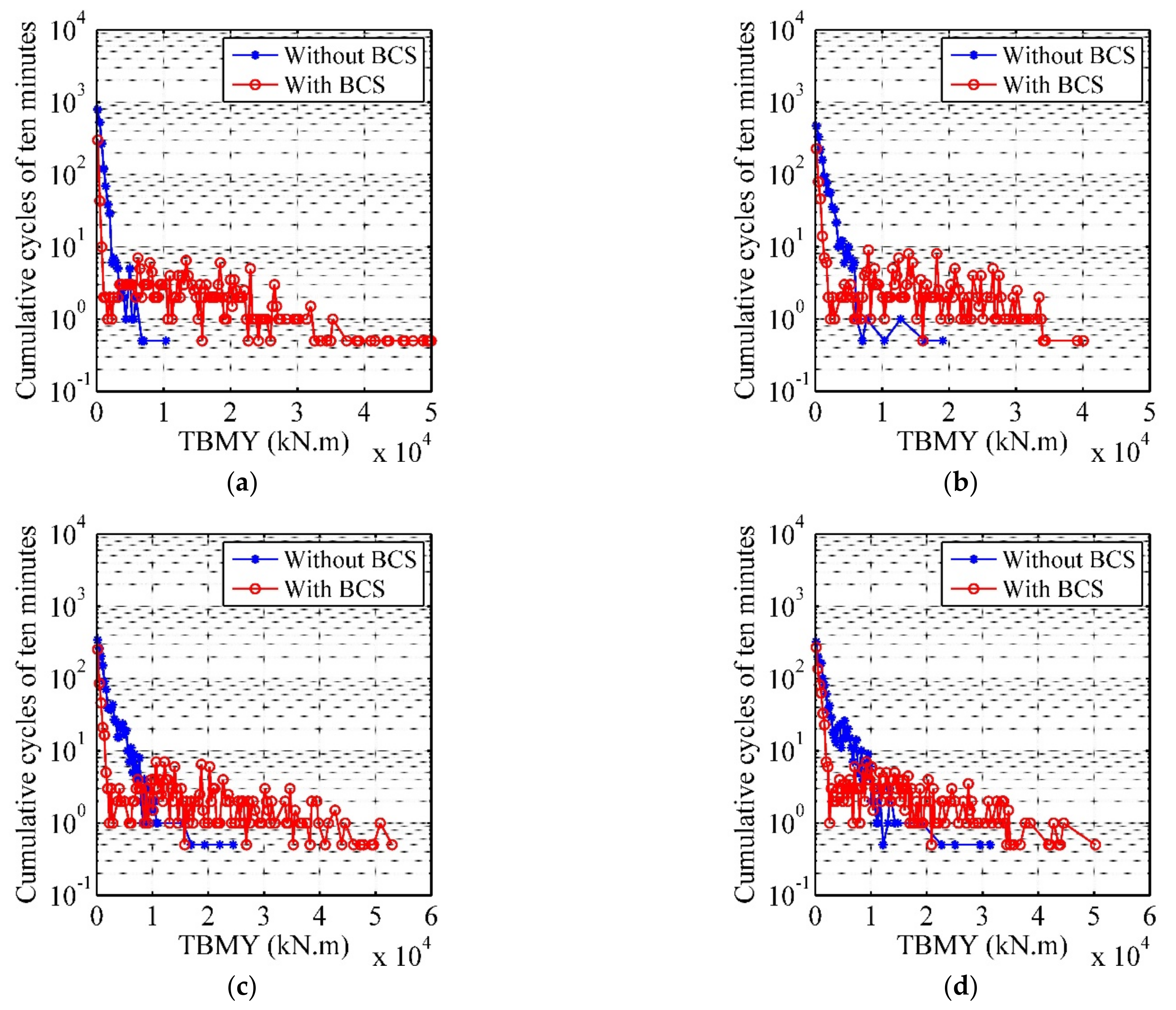
According to Equation (14), it is necessary for fatigue analysis to calculate the rainflow cycles based on the algorithm of rainflow counting [32]. In order to research the effect of BCS on number of rainflow cycles, we binned the fatigue cycle counts according to load range. The width of shear force (BFX and TBFX) and moment (BMY and TBMY) range bins are 20 kN and 300 kN∙m, respectively. And the number of cumulative cycles in the simulated ten minutes for each wind condition can be obtained. According to the analysis in Section 4.1, it is found that the influence of the BCS on the structural responses of the wind turbine is more obvious with the wind speed around cut-in speed and after the rated wind speed. In order to clearly reflect the effect of the BCS on the number of rainflow cycles, we chose 3 (cut-in), 11.4 (rated), 17, and 25 m/s (cut-out) four wind conditions and the comparison of binned range rainflow cycles of the four load components between the two cases for four wind scenarios are shown in Figure 10, Figure 11, Figure 12 and Figure 13. It is observed that the number of cycles is large in the low load range and small in the high load range for two cases. In Figure 10 and Figure 11, the number of cycles are similar between the two cases in the region of below-rated wind speed range and the number of cycles in high load range in No. 1 are slightly higher than that in No. 2 in the region of above-rated wind speed range. The reason is that the oscillation increase of aerodynamic loads during normal operation. From Figure 12 and Figure 13, it is noted that in the region of below-rated wind speed range, the number of cycles in No. 1 are smaller than that in No. 2 because of the 3P of the rotor speed is close to the first tower FA natural frequency when the wind speeds are around the cut-in speed and in the above-rated wind speed range, the number of cycles are similar between the two cases for TBFX and the number of cycles in No. 1 are slightly smaller than that in No. 2 for TBMY. It can be concluded that compared with BFX and BMY in blade root, the effect of BCS on the number of rainflow cycles in high load range on TBFX and TBMY in tower base is more obvious.
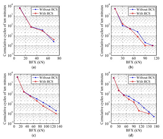
Figure 10.
Comparison of binned range rainflow cycles of BFX between the two cases: (a) Vhub is 3 m/s, (b) Vhub is 11.4 m/s, (c) Vhub is 17 m/s, and (d) Vhub is 25 m/s.
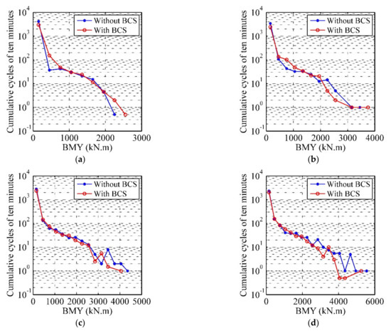
Figure 11.
Comparison of the binned range rainflow cycles of BMY between the two cases: (a) Vhub is 3 m/s, (b) Vhub is 11.4 m/s, (c) Vhub is 17 m/s, and (d) Vhub is 25 m/s.

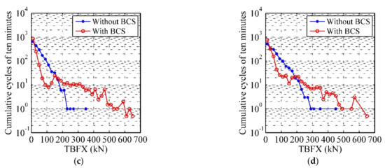
Figure 12.
Comparison of the binned range rainflow cycles of TBFX between the two cases: (a) Vhub is 3 m/s, (b) Vhub is 11.4 m/s, (c) Vhub is 17 m/s, and (d) Vhub is 25 m/s.
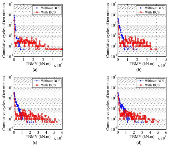
Figure 13.
Comparison of the binned range rainflow cycles of TBMY between the two cases: (a) Vhub is 3 m/s, (b) Vhub is 11.4 m/s, (c) Vhub is 17 m/s, and (d) Vhub is 25 m/s.
4.2.2. Effect of the BCS on DELs
The DELs of the four load components were calculated from the load’s cycles with an alpha version of Mlife, a damaging loads assessment code developed at NREL [43]. In Equation (16), we also find that the load amplitude has a great effect on the DEL. In order to quantify the amount of variation or dispersion of a set of data values, the coefficient of variation (COV) is used. Therefore, the COVs of the four load components were also calculated to analyze the results of the structural dynamic responses in the two cases.
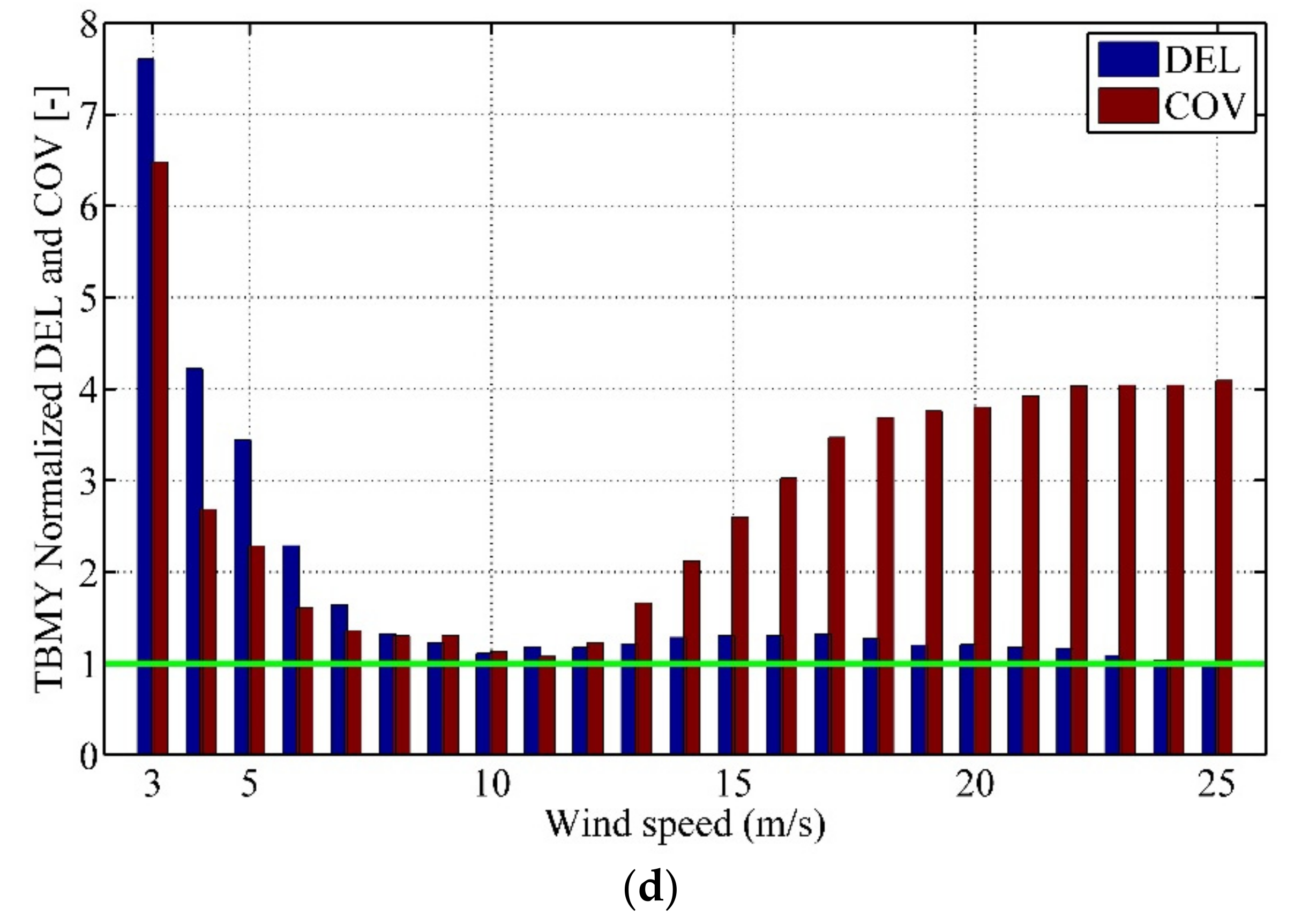
Figure 14 shows the DEL and COV calculation results in different wind scenarios for two cases and compared with No. 1 data as reference values. It can be seen that the values of DEL and COV in No. 2 are larger than that in No. 1 in most conditions, especially for TBFX and TBMY around the cut-in speed. The variation trend of fatigue loads and the related COV as wind speed increase in the region of below-rated wind speed range is consistent, a low COV results in a low DEL and a high COV results in a high DEL. In the region of above-rated wind speed range, because that the volatility in No. 2 is greater than in No. 1 and the mean value of dynamic response in No. 2 is smaller than in No. 1, the normalized COV is significantly larger in DEL in the same wind condition. Figure 14a,b show that the DELs of BFX and BMY in both cases are approximately the same in the region of below-rated wind speed range. However, when the wind speed exceeds the rated speed, the DELs of BFX and BMY in No. 1 are smaller than that in No. 2, which achieves DELs decrease of more than 34% in the cut-out wind speed compared to the No. 2. The changing rotor speeds and blade-pitch angles along time in No. 2 lead to an oscillation increase of aerodynamic loads on the blade which in turn increase the COVs of load components in blade and the load amplitudes in rainflow cycle counting, and then affects the DELs of wind turbine blade. Figure 14c,d shows that the DELs of TBFX and TBMY in No. 2 are greatly larger than that in No. 1 when the wind speeds are around the cut-in speed. The phenomenon is also caused by the reason that the first tower FA natural frequency is close to the 3P of the rotor speed in these wind ranges. When the wind speeds exceed rated speed, the DELs of TBFX in No. 2 are slightly less than that in No. 1 (Figure 14c), while the DELs of TBMY in No. 2 are slightly larger than that in No. 1 (Figure 14d).
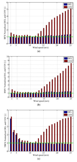

Figure 14.
Comparison the DEL and COV results of No. 2 normalized to No. 1: (a) BFX, (b) BMY, (c) TBFX, and (d) TBMY.
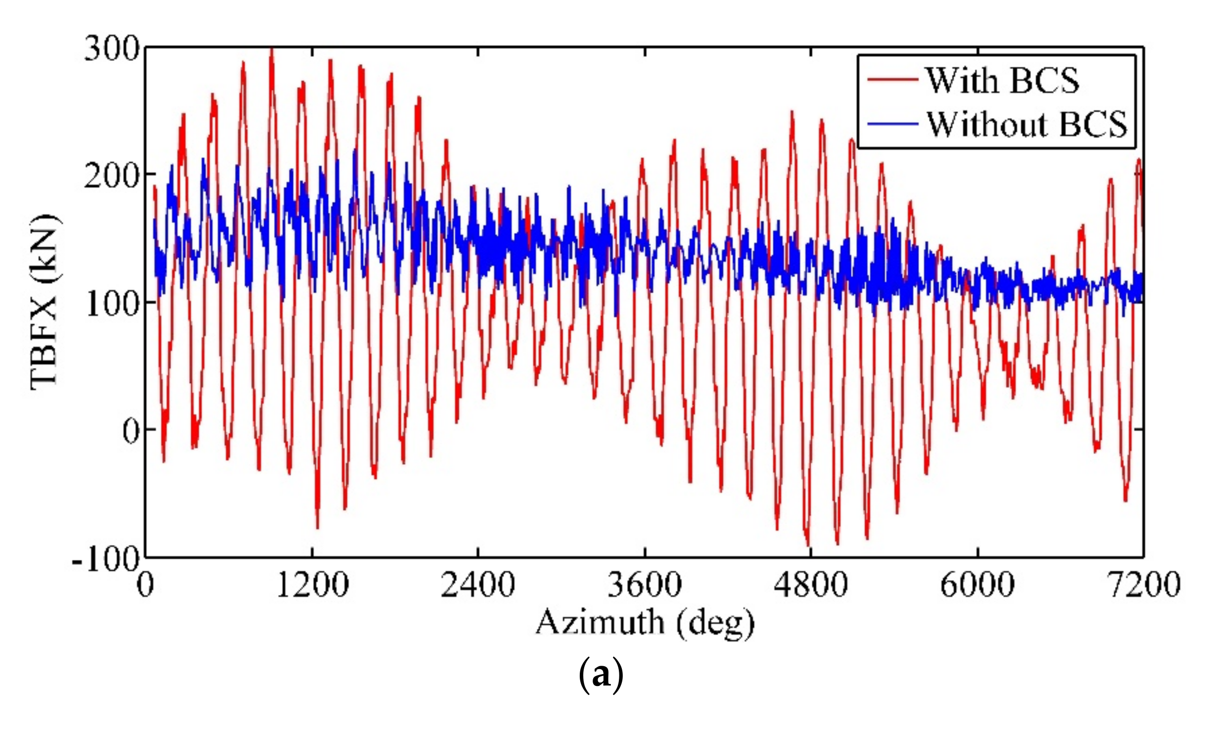
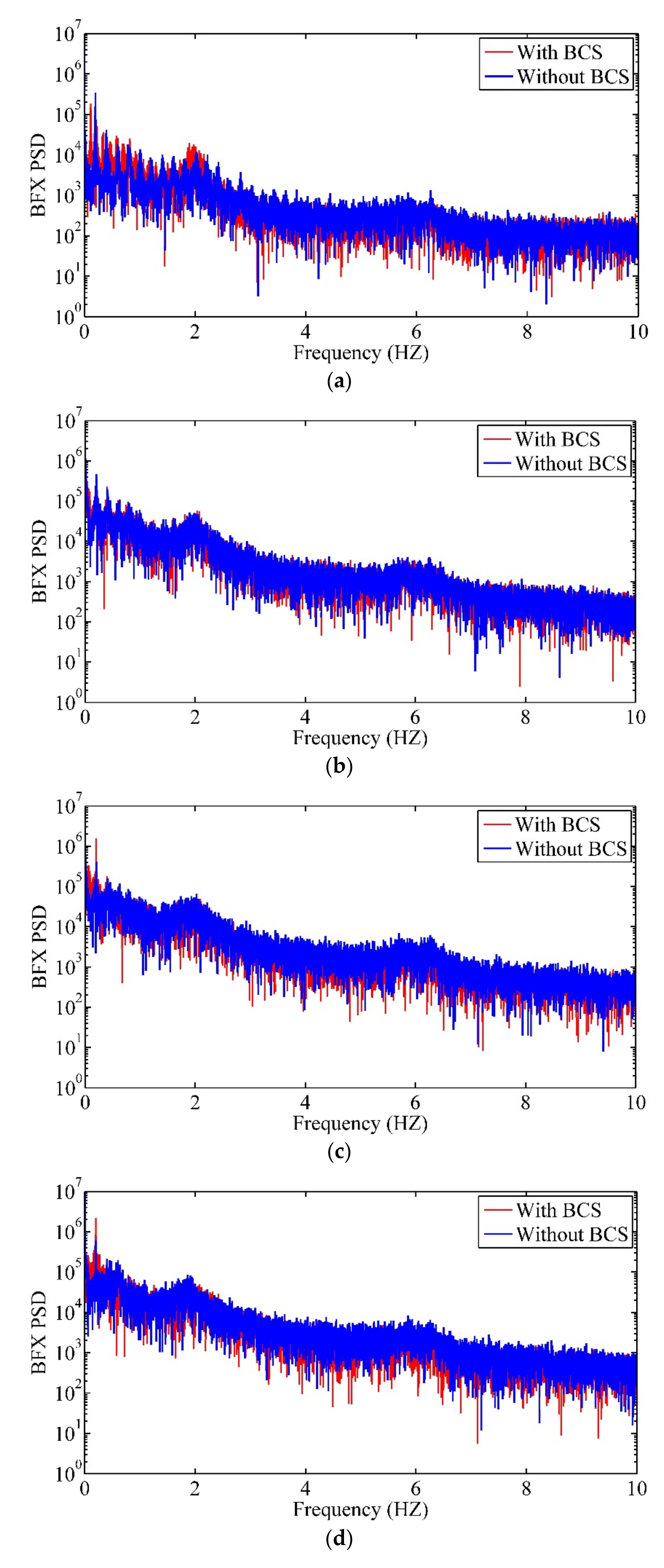
The dynamics are generated from the rotation of the blades in the azimuth direction and the vibrations in the flap-wise and edge-wise directions. Considering that blade’s azimuth position is of great influence on the sinusoidal behavior of blade’s loads and deflections [53], and in order to further analyze the effect of BCS on fatigue loads of blades and tower, the comparison of BFX and TBFX are shown with the azimuth position of the blade in Figure 15 and Figure 16. It can be seen from the figures that under normal operation, the responses of the wind turbine with different azimuth angles in No. 2 fluctuates greatly, which clearly clarify the obvious influence of BCS on fatigue loads of blades and tower. Frequency analysis had been made for BFX and TBFX, and the results are shown in Figure 17 and Figure 18. The pictures show the frequency distribution characteristics under different wind speeds for two cases. And the resonance can be checked in No. 2 from Figure 18a. It is concluded that the BCS should be considered when calculating the fatigue loads of wind turbine blades and support structure subjected to external loads.
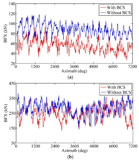
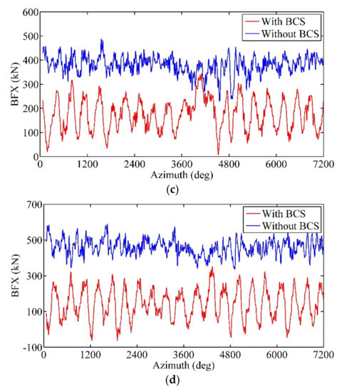
Figure 15.
Comparison of BFX between the two cases: (a) Vhub is 3 m/s, (b) Vhub is 11.4 m/s, (c) Vhub is 17 m/s, and (d) Vhub is 25 m/s.

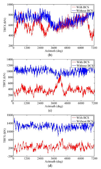
Figure 16.
Comparison of TBFX between the two cases: (a) Vhub is 3 m/s, (b) Vhub is 11.4 m/s, (c) Vhub is 17 m/s, and (d) Vhub is 25 m/s.
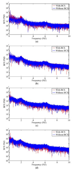
Figure 17.
Comparison of frequency analysis for BFX between the two cases: (a) Vhub is 3 m/s, (b) Vhub is 11.4 m/s, (c) Vhub is 17 m/s, and (d) Vhub is 25 m/s.
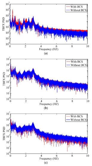
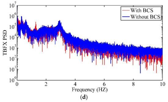
Figure 18.
Comparison of frequency analysis for TBFX between the two cases: (a) Vhub is 3 m/s, (b) Vhub is 11.4 m/s, (c) Vhub is 17 m/s, and (d) Vhub is 25 m/s.
5. Conclusions
This paper investigated the effect of BCS on dynamic and fatigue characteristics of modern wind turbines. Considering the increase of the slenderness ratio and the flexibility of wind turbine in the development of wind energy, it is very significant for the safety of wind turbine structure to accurately calculate the wind-induced dynamic responses of the support structure and blades. Based on FAST code, two different cases with BCS and without BCS are simulated with various wind conditions, from cut-in to cut-out wind speed.
By comparing the mean and maximum values of wind turbine dynamic responses between the two cases, we found that the mean values of the displacement and load components increase with the increase of wind speed in No. 1, while the mean values increase below the rated wind speed and then decrease over the rated wind speed in No. 2, and there are mean values reductions of over 68% in No. 2 at the cut-out wind speed compared to No. 1. The maximum values of the displacement and load components have the same trend with the mean values in the two cases except for the simulation results of tower when the wind speeds are around the cut-in speed. There are maximum values reductions of over 42% in the cut-out wind speed in No. 2 compared to No. 1. To more accurately describe the relationship between the wind speeds and structural dynamic responses when the BCS working, the corresponding fitted curves are carried out and provided, which is helpful to better understand the dynamic features of wind turbine subjected to wind loads during normal operation. In the cut-in wind speed range for No. 2, the 3P of the rotor speed is close to the first tower FA natural frequency, which causes the increase of structural dynamic responses and fatigue loads of the tower when compared to No. 1. By comparing the binned range rainflow cycles of the four load components between the two cases, we found that compared with BFX and BMY, the effect of BCS on the number of rainflow cycles in the high load range on TBFX and TBMY is more obvious. By comparing the COVs and DELs of major load components between the two cases, we found that values of DEL and COV in No. 2 are larger than those in No. 1 in most conditions, especially for TBFX and TBMY around the cut-in speed. In addition, the obvious influence of BCS was clarified by comparing the BFX and TBFX with the azimuth position of the blade and frequency analysis between the two cases for four typical wind scenarios.
According to the simulation results, it is concluded that the traditional method analyzing the dynamic responses of wind turbine blades and tower without considering the BCS will overestimate the mean and maximum values of structural responses while underestimate the fatigue loads. Therefore, to improve the safety and reliability of wind turbine structure, the BCS should be considered for design, structural dynamics, and fatigue analysis. Since the BCS plays an important role in the safe operation of modern wind turbines, future research efforts can be focused on BCS optimization, such as the influence of Tip Speed Ratio on control results and a more effective fatigue analysis method.
Author Contributions
Conceptualization, methodology, software, validation, formal analysis, investigation, data curation, writing original draft, C.Y.; supervision, writing-review and editing, J.L.; supervision, writing-review, and editing, Y.X.; supervision, methodology, W.B.; Methodology, J.W. All authors have read and agreed to the published version of the manuscript.
Funding
This research was funded by the Key Research and Development and Promotion Project in Henan Province (Grant No. 212102310269), National Natural Science Foundation of China (Grant No. 51679092) and Scientific Research Project of North China University of Water Resources and Electric Power (Grant No. 201811007).
Institutional Review Board Statement
Not applicable.
Informed Consent Statement
Not applicable.
Data Availability Statement
Data underlying the results presented in this paper are not publicly available at this time but may be obtained from the authors upon reasonable request.
Acknowledgments
We are grateful for the support and the help of Jonkman for providing FAST code.
Conflicts of Interest
The authors declare no conflict of interest.
References
- Lee, J.; Zhao, F. Global Wind Report 2021; Global Wind Energy Council (GWEC): Brussels, Belgium, 2021. [Google Scholar]
- Moné, C.; Hand, M.; Bolinger, M.; Rand, J.; Heimiller, D.; Ho, J. 2015 Cost of Wind Energy Review; National Renewable Energy Lab. (NREL): Golden, CO, USA, 2017. [Google Scholar]
- Martin, O.L.H. Aerodynamics of Wind Turbines, 3rd ed.; Routledge: London, UK, 2015. [Google Scholar]
- Thirstrup, P.J. Kinematically Nonlinear Finite Element Model of a Horizontal Axis Wind Turbine. Part 1. Mathematical Model and Results. Ph.D. Thesis, Risoe National Lab., Roskilde, Denmark, 1 July 1990. [Google Scholar]
- Naguleswaran, S. Lateral vibration of a centrifugally tensioned uniform Euler-Bernoulli beam. J. Sound Vib. 1994, 176, 613–624. [Google Scholar] [CrossRef]
- Baumgart, A. A mathematical model for wind turbine blades. J. Sound Vib. 2002, 251, 1–12. [Google Scholar] [CrossRef]
- Kiyomiya, O.; Rikiji, T.; van Gelder, P.H. Dynamic response analysis of onshore wind energy power units during earthquakes and wind. In Proceedings of the Twelfth International Offshore and Polar Engineering Conference, Kitakyushu, Japan, 26–31 May 2002. [Google Scholar]
- Murtagh, P.J.; Basu, B.; Broderick, B.M. Along-wind response of a wind turbine tower with blade coupling subjected to rotationally sampled wind loading. Eng. Struct. 2005, 27, 1209–1219. [Google Scholar] [CrossRef]
- Kallesøe, B.S. Equations of motion for a rotor blade, including gravity, pitch action and rotor speed variations. Wind. Energy Int. J. Prog. Appl. Wind. Power Convers. Technol. 2007, 10, 209–230. [Google Scholar] [CrossRef]
- Chen, X.; Li, J.; Chen, J. Wind-induced response analysis of a wind turbine tower including the blade-tower coupling effect. J. Zhejiang Univ. Sci. A 2009, 10, 1573–1580. [Google Scholar] [CrossRef]
- Li, J.; Chen, J.; Chen, X. Aerodynamic response analysis of wind turbines. J. Mech. Sci. Technol. 2011, 25, 89–95. [Google Scholar] [CrossRef]
- Gebhardt, C.G.; Roccia, B.A. Non-linear aeroelasticity: An approach to compute the response of three-blade large-scale horizontal-axis wind turbines. Renew. Energy 2014, 66, 495–514. [Google Scholar] [CrossRef]
- Guo, S.; Li, Y.; Chen, W. Analysis on dynamic interaction between flexible bodies of large-sized wind turbine and its response to random wind loads. Renew. Energy 2021, 163, 123–137. [Google Scholar] [CrossRef]
- Shkara, Y.; Schelenz, R.; Jacobs, G. The Effect of Blade-Tower Interaction on the Structure Loading of Multi Megawatt Horizontal Axis Wind Turbine; Journal of Physics Conference Series; IOP Publishing: Bristol, UK, 2018; Volume 1037, p. 072033. [Google Scholar]
- Feliciano, J.; Cortina, G.; Spear, A.; Calaf, M. Generalized analytical displacement model for wind turbine towers under aerodynamic loading. J. Wind. Eng. Ind. Aerodyn. 2018, 176, 120–130. [Google Scholar] [CrossRef]
- Hu, Y.; Yang, J.; Baniotopoulos, C.; Wang, X.; Deng, X. Dynamic analysis of offshore steel wind turbine towers subjected to wind, wave and current loading during construction. Ocean. Eng. 2020, 216, 108084. [Google Scholar] [CrossRef]
- Banerjee, A.; Chakraborty, T.; Matsagar, V.; Achmus, M. Dynamic analysis of an offshore wind turbine under random wind and wave excitation with soil-structure interaction and blade tower coupling. Soil Dyn. Earthq. Eng. 2019, 125, 105699. [Google Scholar] [CrossRef]
- Nezamolmolki, D.; Shooshtari, A. Investigation of nonlinear dynamic behavior of lattice structure wind turbines. Renew. Energy 2016, 97, 33–46. [Google Scholar] [CrossRef]
- Feyzollahzadeh, M.; Mahmoodi, M.J.; Yadavar-Nikravesh, S.M.; Jamali, J. Wind load response of offshore wind turbine towers with fixed monopile platform. J. Wind. Eng. Ind. Aerodyn. 2016, 158, 122–138. [Google Scholar] [CrossRef]
- Pim, V.D.M.; Karel, N.V.D.; Andrei, V.M. The effect of the nonlinear velocity and history dependencies of the aerodynamic force on the dynamic response of a rotating wind turbine blade. J. Sound Vib. 2016, 383, 191–209. [Google Scholar]
- Kong, C.; Bang, J.; Sugiyama, Y. Structural investigation of composite wind turbine blade considering various load cases and fatigue life. Energy 2005, 30, 2101–2114. [Google Scholar] [CrossRef]
- Kong, C.; Kim, T.; Han, D. Investigation of fatigue life for a medium scale composite wind turbine blade. Int. J. Fatigue 2006, 28, 1382–1388. [Google Scholar] [CrossRef]
- Shokrieh, M.M.; Rafiee, R. Simulation of fatigue failure in a full composite wind turbine blade. Compos. Struct. 2006, 74, 332–342. [Google Scholar] [CrossRef]
- Do, T.Q.; van de Lindt, J.W.; Mahmoud, H. Fatigue life fragilities and performance-based design of wind turbine tower base connections. J. Struct. Eng. 2015, 141, 04014183. [Google Scholar] [CrossRef]
- Lee, H.G.; Kang, M.G.; Park, J. Fatigue failure of a composite wind turbine blade at its root end. Compos. Struct. 2015, 133, 878–885. [Google Scholar] [CrossRef]
- Summary of Wind Turbine Accident Data to 30 June 2021. Available online: http://www.caithnesswindfarms.co.uk/AccidentStatistics.htm (accessed on 1 August 2021).
- Jonkman, J.M.; Buhl, J.M.L. FAST User’s Guide; National Renewable Energy Laboratory: Golden, CO, USA, 2005; Volume 365, p. 366. [Google Scholar]
- Yuan, C.; Chen, J.; Li, J.; Xu, Q. Fragility analysis of large-scale wind turbines under the combination of seismic and aerodynamic loads. Renew. Energy 2017, 113, 1122–1134. [Google Scholar] [CrossRef]
- Yuan, C.; Chen, J.; Li, J.; Xu, Q.; Xie, Y. Study on the influence of baseline control system on the fragility of large-Scale wind turbine considering seismic-aerodynamic combination. Adv. Civ. Eng. 2020, 2020, 8471761. [Google Scholar] [CrossRef]
- Li, H.; Hu, Z.; Wang, J.; Meng, X. Short-term fatigue analysis for tower base of a spar-type wind turbine under stochastic wind-wave loads. Int. J. Nav. Archit. Ocean. Eng. 2018, 10, 9–20. [Google Scholar] [CrossRef]
- Jonkman, J.M.; Butterfield, S.; Musial, W.; Scott, G. Definition of a 5-MW Reference Wind Turbine for Offshore System Development; National Renewable Energy Lab. (NREL): Golden, CO, USA, 2009. [Google Scholar]
- Kane, T.R.; Levinson, D.A. Dynamics, Theory and Application; McGraw Hill: New York, NY, USA, 1985. [Google Scholar]
- Jonkman, J.M. Modeling of the UAE Wind Turbine for Refinement of FAST_AD; National Renewable Energy Lab.: Golden, CO, USA, 2003. [Google Scholar]
- Jonkman, J.; Buhl, M. New developments for the NWTC’s fast aeroelastic HAWT simulator. In Proceedings of the 42nd AIAA Aerospace Sciences Meeting and Exhibit, Reno, NV, USA, 5–8 January 2004; p. 504. [Google Scholar]
- Chen, J.; Yuan, C.; Li, J.; Xu, Q. Semi-active fuzzy control of edgewise vibrations in wind turbine blades under extreme wind. J. Wind. Eng. Ind. Aerodyn. 2015, 147, 251–261. [Google Scholar] [CrossRef]
- Wright, A.D.; Fingersh, L.J. Advanced Control Design for Wind Turbines; Part I: Control Design, Implementation, and Initial Tests; National Renewable Energy Lab. (NREL): Golden, CO, USA, 2008. [Google Scholar]
- Available online: https://www.nrel.gov/wind/nwtc/fast.html (accessed on 4 March 2022).
- International Electrotechnical Commission. Wind Turbines-Part 1: Design Requirements, 3rd ed.; IEC 61400-1; International Electrotechnical Commission: Geneva, Switzerland, 2005. [Google Scholar]
- Ismaiel, A.M.M.; Yoshida, S. Study of turbulence intensity effect on the fatigue lifetime of wind turbines. Evergreen 2018, 5, 25–32. [Google Scholar] [CrossRef]
- Jonkman, B.J. TurbSim User’s Guide: Version 1.50; National Renewable Energy Lab. (NREL): Golden, CO, USA, 2009. [Google Scholar]
- Downing, S.D.; Socie, D.F. Simple rainflow counting algorithms. Int. J. Fatigue 1982, 4, 31–40. [Google Scholar] [CrossRef]
- Manwell, J.F.; McGowan, J.G.; Rogers, A.L. Wind Energy Explained: Theory, Design and Application; John Wiley & Sons: Hoboken, NJ, USA, 2010. [Google Scholar]
- Hayman, G.J.; Buhl, M., Jr. Mlife Users Guide for Version 1.00; National Renewable Energy Laboratory: Golden, CO, USA, 2012; Volume 74, p. 112. [Google Scholar]
- Girsang, I.P.; Dhupia, J.S. Pitch controller for wind turbine load mitigation through consideration of yaw misalignment. Mechatronics 2015, 32, 44–58. [Google Scholar] [CrossRef]
- Aho, J.; Pao, L.Y.; Fleming, P. Controlling Wind Turbines for Secondary Frequency Regulation: An Analysis of AGC Capabilities under New Performance based Compensation Policy; National Renewable Energy Lab. (NREL): Golden, CO, USA, 2015. [Google Scholar]
- Karlina-Barber, S.; Mechler, S.; Nitschke, M. The effect of wakes on the fatigue damage of wind turbine components over their entire lifetime using short-term load measurements. J. Phys. Conf. Ser. 2016, 753, 072022. [Google Scholar] [CrossRef] [Green Version]
- Schafhirt, S.; Page, A.; Eiksund, G.R.; Muskulus, M. Influence of soil parameters on the fatigue lifetime of offshore wind turbines with monopile support structure. Energy Procedia 2016, 94, 347–356. [Google Scholar] [CrossRef] [Green Version]
- Malcolm, D.J.; Hansen, A.C. WindPACT Turbine Rotor Design Study; National Renewable Energy Laboratory: Golden, CO, USA, 2002. [Google Scholar]
- Genta, G. A fast modal technique for the computation of the Campbell diagram of multi-degree-of-freedom rotors. J. Sound Vib. 1992, 155, 385–402. [Google Scholar] [CrossRef]
- Ritto, T.G.; Lopez, R.H.; Sampaio, R. Robust optimization of a flexible rotor-bearing system using the Campbell diagram. Eng. Optim. 2011, 43, 77–96. [Google Scholar] [CrossRef]
- Yang, J.; Song, D.; Dong, M.; Chen, S.; Zou, L.; Guerrero, J.M. Comparative studies on control systems for a two-blade variable-speed wind turbine with a speed exclusion zone. Energy 2016, 109, 294–309. [Google Scholar] [CrossRef] [Green Version]
- Wandji, W.N.; Natarajan, A.; Dimitrov, N. Development and design of a semi-floater substructure for multi-megawatt wind turbines at 50+ m water depths. Ocean. Eng. 2016, 125, 226–237. [Google Scholar] [CrossRef]
- Ismaiel, A.; Yoshida, S. Aeroelastic analysis of a coplanar twin-rotor wind turbine. Energies 2019, 12, 1881. [Google Scholar] [CrossRef] [Green Version]


Publisher’s Note: MDPI stays neutral with regard to jurisdictional claims in published maps and institutional affiliations. |
© 2022 by the authors. Licensee MDPI, Basel, Switzerland. This article is an open access article distributed under the terms and conditions of the Creative Commons Attribution (CC BY) license (https://creativecommons.org/licenses/by/4.0/).