Thermal–Structural Coupling Analysis of Subsea Connector Sealing Contact

Abstract

Taking a subsea collet connector as an example, the contact characteristics of the sealing structure of the subsea connector under thermal–structural coupling were studied. Considering the heat transfer problem of the subsea connector in deep water, the heat transfer model of seawater layer between sealing structures was established, and the relationship between equivalent thermal conductivity, composite heat transfer coefficient, and temperature was determined. The steady-state temperature field distribution of the connector under the action of the internal high-temperature oil and gas and external low-temperature seawater was obtained. Considering the stress and deformation of the subsea connector under the thermal load, the thermal–structural coupling analysis model of the steady-state temperature field was established, and the thermal stress theoretical analysis and numerical simulation of the key sealing structures of the connector were compared and verified. Analysis of coupled stress calculation, for example, under a steady-state temperature field, was carried out on the sealing structure of the subsea connector. At the same time, the pressure shock mode under a steady temperature field was analyzed, which showed that the lenticular sealing gasket is sensitive to high pressure under high-temperature conditions.

1. Introduction

The connection and sealing technology between the equipment of subsea production systems in the deep-water oil and gas field is an internationally recognized technical problem [1]. The sealing contact performance of the subsea connector determines the success or failure of the connection. In particular, the temperature characteristics of the sealing structure under the action of internal high-temperature oil and gas and external low-temperature seawater are among the fundamental factors for the long-term reliable operation of the connector. The sealing structure is subjected to the combined action of external force and temperature load during underwater work, and it is very easy to produce excessive deformation of the contact surface, which affects the sealing performance [2]. Therefore, it is necessary to conduct thermal–structural coupling analysis of the contact surface of the sealing structure of the subsea connector.

Scholars have done a lot of research on the contact under a structural load or temperature load. In 2007, Abid M et al. [3] analyzed the sealing performance of flange connectors under variable steady-state thermal load and thermal transient load and studied the relationship between the contact pressure of the sealing hub, stress relaxation of the bolt, etc., and the temperature load. Zhou Xianjun et al. [4] studied the heat transfer model of a bolted flange connection based on the nonlinearity of gaskets, obtained the distribution of the transient temperature field of the hub, and then analyzed the influence of transient temperature field changes on the bolt load and gasket stress. Al-Turki LI et al. [5] found that the bending strength of composite materials under bending loads mainly depends on the medium and the aging degree, and the decrease in bending strength under contact load is mainly due to the increase in the number of contact cycles. Avanzani A and Donzella G [6] combined the equivalent strain range calculated at the critical point of the seal with the life curve of the material to calculate the fatigue damage and working life of the sealing material in ultra-high pressure applications. In 2009, Omiya Yuya et al. [7] analyzed the thermal stress of bolted flanges under internal pressure and heat conduction conditions and proved that the sealing performance of the bolted flange structure increased with the increase in temperature based on numerical simulation and experiments. In 2015, Sawa T et al. [8] conducted many experiments on the sealing performance of the bolt flange at high temperature, obtained the compression–resilience performance and thermal expansion coefficient of sealing gasket at different temperatures, and carried out experimental verification. In 2016, Luo Yan-Yan et al. [9] studied the influence of heat differences and the temperature alteration ratio on the degeneration of aviation electrical connector performance in thermal fatigue experiments based on the theory of accelerated life experiments and analyzed the failure mechanism of thermal fatigue. In 2018, Wang Lu et al. [10] analyzed the axial bolt force, maximum bolt stress, and gasket contact stress during steady and transient heat processes and found that the maximum bolt stress was proportional to the temperature, while the average gasket contact stress was inversely proportional to the temperature. In addition, the heating rate significantly affected the maximum stress of bolts and gasket contact stress. Abdullah Oday Ibraheem et al. [11] used an axisymmetric model for numerical analysis to simulate the engagement of the single-disc friction clutch system and used a sequential thermo-mechanical coupling method to analyze the thermal stress of the automobile clutch under dry conditions. The research results showed that contact pressure had a significant influence on the thermal stress in both sliding and heating stages. In 2019, Zhang Lanzhu et al. [12] analyzed the stress distribution of metal-to-metal contact flange connections under different pressures, temperatures, and bending moments based on the finite element method and showed that under different thermal loads, when the initial bolt stress was sufficient to reach the metal-to-metal contact, the maximum bending moment that the connection could withstand was determined by strength criteria. In 2019, Tang Liping et al. [13] found that the sealing performance of a metal polymer interface had more complex characteristics. Temperature has an important impact on the thermal deformation of the sealing structure in the temperature field, and an appropriate high temperature can improve the sealing ability. In 2020, Chen Jinlin et al. [14] considered the elastic deformation and thermal stress deformation of the micro-convex body based on fractal theory and analyzed the normal contact stiffness of the double friction interface of dry gas seals. These authors obtained the influence of the fractal dimension and characteristic dimension on the thermal and elastic normal contact stiffness, that is, the former had a positive ratio, and the latter was inversely proportional. Wang Qiang et al. [15] established a fluid dynamics and heat transfer model of porous media through the thermal stress module of the ANSYS Workbench, corrected the friction heating model, and calculated the thermal deformation of fingers according to the pressure and temperature results.

As can be seen from the above literature review, previous researchers mainly studied the mechanical properties of the seal structure under thermal–structural coupling and the structural contact stress under external load or thermal stress. However, the contact state and mechanical characteristics of the sealing structure under the action of thermal stress and structural stress were not considered sufficiently. Therefore, this paper analyzes the heat transfer process when the subsea connector is subjected to the action of internal high-temperature oil and external low-temperature seawater and simplifies the heat transfer by equivalent thermal conductivity and the composite heat transfer coefficient. The structural stress of the subsea connector under a mechanical load and thermal stress produced by temperature loads is coupled to analyze the contact characteristics and overall stress change of the subsea connector lenticular sealing structure in the thermal–structural coupling field. Because the contact stress of the sealing contact surface cannot be analyzed by a sticking strain gauge, the correctness of this method was verified by comparing the finite element numerical simulation with the theoretical analysis.

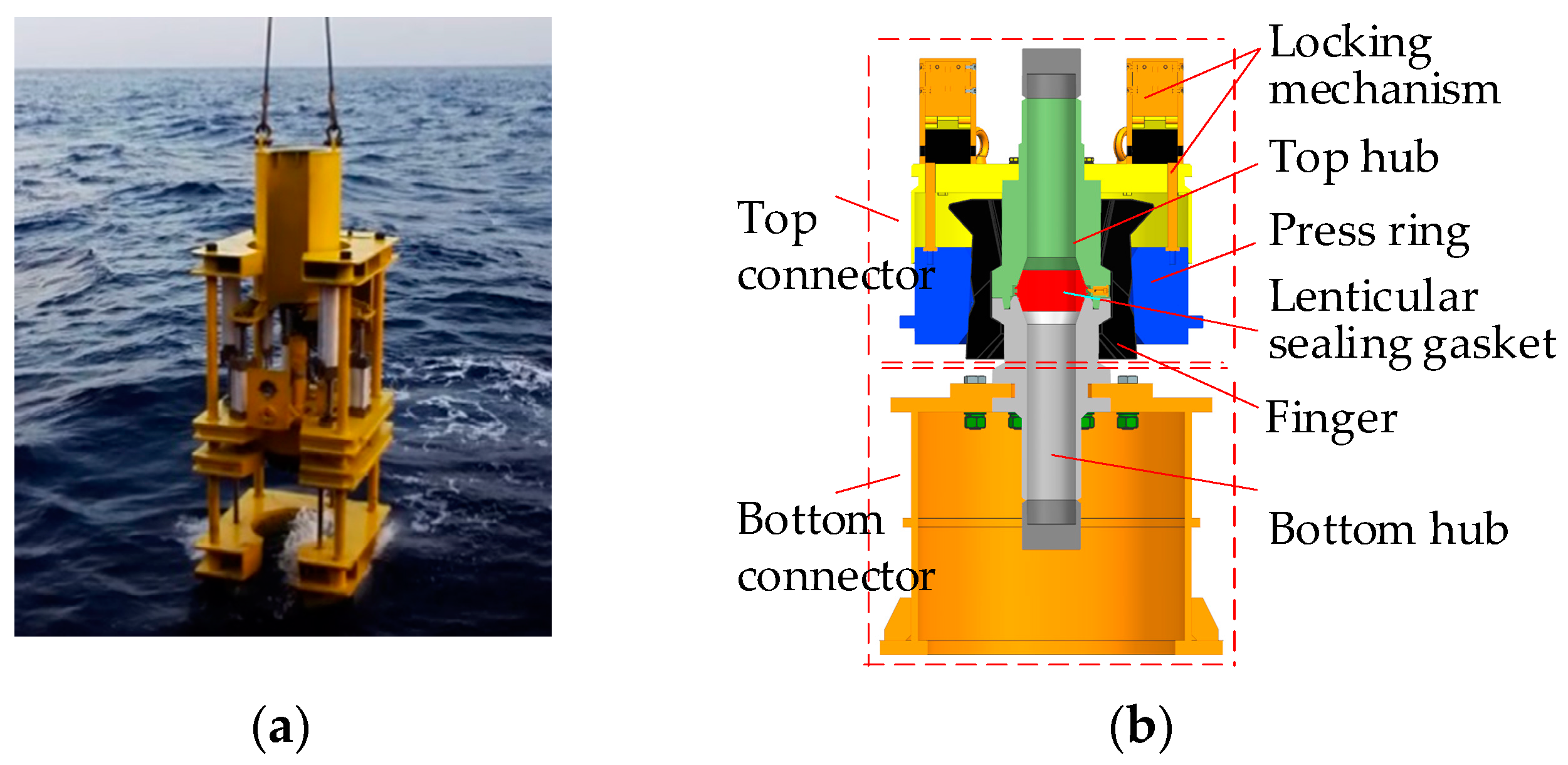
2. The Structure of the Subsea Connector

The metal lenticular sealing gasket is usually used as the main seal for the subsea collect connector and clamp-type connector, which are commonly used in deep sea environments. This article takes the subsea collect connector as an analysis case, as shown in Figure 1. The core sealing structure of the subsea collect connector is composed of a lenticular sealing gasket, top hub, and bottom hub. The external installation tool drives the press ring to move downward to make the fingers clasp the top and bottom hubs and exert pre-tightening force on the sealing structure to complete the connection and sealing. In the whole structure, the parts directly exposed to the oil and gas medium include the top hub, bottom hub, and lenticular sealing gasket. Therefore, these three parts are greatly affected by the change in the temperature load. The applicable range of underwater temperature of the whole underwater connector system is 3~150 °C, which is also the temperature load change range of the subsea connector thermal structure coupling analysis in this paper. When the sealing structure of the subsea connector is subjected to external load and temperature load, the structural stress and thermal stress will overlap. If the coupling stress is too large, it will have an irreversible impact on the sealing structure, especially on the sealing contact surface. Therefore, the mechanical and sealing contact characteristics of the sealing structure of the subsea connector under the thermal–structural coupling effect should be analyzed in detail.

3. Research on the Heat Transfer Model of the Subsea Connector

The subsea connector works at a relatively constant temperature. If the temperature of oil and gas inside the connector tends to be constant, the temperature of the components from the inside to the outside of the connector will also be constant, which is regarded as the steady-state temperature distribution. According to the second law of thermodynamics, subsea connectors are generally subjected to the action of internal high-temperature oil and gas and external low-temperature seawater during operation, so there must be heat transfer problems. The basic heat transfer modes of the subsea connector are thermal conduction, thermal convection, and thermal radiation.

As shown in Figure 2, the heat transfer model of the subsea connector was used to analyze the temperature field distribution of the sealing structure. In the finite element analysis of the ANSYS Workbench, the calculation methods of the three heat transfer modes are different. Among them, the thermal conduction is close to linear and is relatively simple; the convective heat transfer coefficient cannot be directly obtained, which increases the difficulty of applying boundary conditions; and the thermal radiation is proportional to the fourth power of the object temperature, so its finite element analysis is highly nonlinear, and its convergence cannot be guaranteed by direct calculation. Therefore, it is necessary to establish the corresponding heat transfer model. When establishing a heat transfer model, structural characteristics and calculation accuracy should be considered at the same time, and heat transfer factors that have little influence should be ignored. The heat transfer mode should be simplified, and equivalent thermal conductivity and composite thermal conductivity should be introduced to facilitate the application of boundary conditions. The temperature of the medium inside the subsea connector: at low temperature, the medium temperature is seawater temperature, and at high temperature, the medium temperature is oil and gas temperature; at the same time, the heat transfer coefficients of the internal and external fluid media can be obtained, so the third boundary condition of heat transfer is satisfied [16,17].

3.1. Heat Transfer Model of the Seawater Layer between the Hub and Collet

Figure 3 shows a simplified cross-sectional view of the position relationship between the hub and the collet. The seawater layer between the hub and the collet is very thin, but not negligible, otherwise, the temperature difference between the hub and the collet will increase. Since the hub outer surface and the collet inner surface are not flat, the introduced shape factor represents the energy flux between the two surfaces. Firstly, the energy exchange between the area elements of the two surfaces is obtained, and then the integral of the two surfaces is determined. Therefore, the shape factor is mainly related to the geometric state of the two surfaces. In addition, the shape factor only represents the percentage of radiative transfer on one surface and has nothing to do with the energy absorption capacity of the other surface. The heat transfer model between the hub and the collet can be simplified as the heat transfer problem between two concentric cylinders. As shown in Figure 3, L₁ is the height of the seawater layer. ε is the emissivity, 0 ≤ ε ≤ 1; $\sigma$ is the Stephen-Boltzmann constant; A₁ is the area of the smaller surface, set as surface 1; T₁ is the temperature of surface 1; T₂ is the larger surface (set as the temperature of surface 2); φ_1–2 is the shape factor from surface 1 to surface 2. The radiation shape factor [18,19] of the hub and collet surface is

$${\phi }_{1-2}=R_1\left[1-\frac{1}{\pi }{\cos }^{-1}\left(\frac{{\chi }_1}{{\chi }_2}\right)\right]+\frac{\sqrt{{({\chi }_1+2)}^2-4R_1^2}}{2\pi R_2}{\cos }^{-1}\left(R_1\frac{{\chi }_1}{{\chi }_2}\right)+\frac{{\chi }_1}{2\pi R_2}{\sin }^{-1}{R}_1-\frac{{\chi }_2}{4R_2}$$

(1)

where r₁ is the outer diameter of the flange; r₂ is the inner diameter of the collet; $R_1=\frac{r_1}{r_2}$; $R_2=\frac{L_1}{r_2}$; ${\chi }_1=R_2^2+R_1^2$ $-1$; ${\chi }_2=R_2^2+R_1^2+1$. Considering the influence of radiation in the system on heat transfer, the emissivity of the system can be obtained, ε_s

$${\epsilon }_s=\frac{1}{1+{\phi }_{1-2}\left(\frac{1}{{\epsilon }_1}-1\right)+{\phi }_{2-1}\left(\frac{1}{{\epsilon }_2}-1\right)}$$

(2)

where ε₁ and ε₂ are the emissivity of the hub and collet. Since the materials selected for each part of the subsea connector are corrosion-resistant alloy steel and heat-resistant alloy steel, during the long-term operation in deep water, they will be corroded by seawater to produce an oxide layer, so the emissivity of each part is taken as 0.8.

The flow of seawater is very slow because the seawater layer is wrapped in the press ring and the wall tube. Therefore, convective heat transfer can be ignored. Accordingly, only two heat transfer methods, thermal conduction and thermal radiation, are considered between the hub and the collet and can be obtained from the energy conservation on the hub surface

$$Q_{1-2}=2\pi L_1\cdot {\lambda }_{k2}\cdot \frac{T_1-T_2}{\ln \left(r_2/r_1\right)}+{\epsilon }_{s}2\pi r_1{L}_1{\phi }_{1-2}{C}_0\left[{\left(\frac{T_1}{100}\right)}_{}^4-{\left(\frac{T_2}{100}\right)}_{}^4\right]$$

(3)

where Q_1–2 is the total heat transferred from the seawater layer between the hub and the collet; λ_k2 is the thermal conductivity of seawater at temperature T₂ [18]; T₁ is the temperature of the hub outer surface (as shown in Figure 3); T₂ is the temperature of the collet inner surface (as shown in Figure 3); C₀ is the black-body radiation coefficient. In the finite element analysis, compared with convective heat transfer and thermal radiation, the calculation and regulation of thermal conduction are easier. Therefore, the equivalent thermal conductivity is defined to describe the entire process of thermal conduction and thermal radiation. The right side of Equation (3) is the total energy transferred under the action of thermal conduction and thermal radiation. Using the equivalent thermal conductivity λ_e1, the heat transfer can be expressed as

$$Q_{1-2}=2\pi L_1{\lambda }_{e1}\frac{T_1-T_2}{\ln \left(r_2/r_1\right)}$$

(4)

Through consideration of Equations (3) and (4) comprehensively, λ_e1, can be expressed as

$${\lambda }_{e1}={\lambda }_{k2}+r_1{\epsilon }_s{\phi }_{1-2}{C}_0\left[{\left(\frac{T_1}{100}\right)}_{}^4-{\left(\frac{T_2}{100}\right)}_{}^4\right]\frac{\ln \left(r_2/r_1\right)}{T_1-T_2}$$

(5)

The relationship between the equivalent thermal conductivity λ_e1 and temperature is shown in Figure 4.

3.2. Heat Transfer Model of the Seawater Layer between the Hub and Lenticular Sealing Gasket

Figure 5a shows a schematic diagram of heat transfer between the hub inner surface and the lenticular sealing gasket. The heat transfer between the hub inner surface and the lenticular sealing gasket includes the thermal conduction q₁ between the lenticular sealing gasket and seawater, the convective heat transfer q₂ of the seawater, and the thermal radiation q₃ from the lenticular sealing gasket to the top and bottom hub.

The gap is narrow and the flow of seawater is extremely low because of the sealing state between the hub and the lenticular sealing gasket. Convective heat transfer on the surface has less influence than thermal conduction and radiative heat transfer, so it can be ignored. As shown in Figure 5b, the model of heat transfer is simplified as a composite heat transfer combining thermal conduction and thermal radiation. The heat transfer quantity of the seawater layer between the lenticular sealing gasket and the hub, Q_3–4, can be expressed as:

$$Q_{3-4}=2\pi L_2\cdot {\lambda }_{k4}\cdot \frac{T_3-T_4}{\ln (r_4/r_3)}+2\pi r_3{\epsilon }_s{L}_2{\phi }_{3-4}{C}_0\left[{\left(\frac{T_3}{100}\right)}^4-{\left(\frac{T_4}{100}\right)}^4\right]$$

(6)

where λ_k4 is the thermal conductivity of seawater at temperature T₄ [18]; T₃ is the temperature of sealing gasket outer surface; T₄ is the temperature of the top hub inner surface; r₃ is the outer diameter of the sealing gasket; r₄ is the inner surface of the hub; C₀ is the black-body radiation coefficient; φ_3–4 is the shape factor from the sealing ring outer surface 3 to the flange inner surface 4, and the calculation method is the same as that in Equation (1). The equivalent thermal conductivity of the heat transfer model, λ_e2, can be expressed as:

$${\lambda }_{e2}={\lambda }_{k4}+r_3{\epsilon }_s{\phi }_{3-4}{C}_0\left[{\left(\frac{T_3}{100}\right)}^4-{\left(\frac{T_4}{100}\right)}^4\right]\frac{\ln (r_4/r_3)}{T_3-T_4}$$

(7)

The relationship between equivalent thermal conductivity λ_e2 and temperature is shown in Figure 6.

3.3. The Heat Transfer Model of the Outer Surface of the Finger and the Press Ring

Since the subsea connector has 12 fingers, the seawater between the fingers and the press ring will flow through the gaps between the fingers. This part of the seawater has strong fluidity, so it can be incorporated into the heat transfer model of the outer surface of the press ring for analysis. The heat transfer model on the outer surface of the press ring is shown in Figure 7.

As shown in Figure 7, the outer surface of the press ring is in direct contact with the flowing seawater, and the main methods of heat transfer are convective heat transfer q₂ generated by the seawater flowing through the outer surface and radiative heat transfer q₃ with the outside world. The convective heat transfer loss, Q_p, can be expressed as:

$$Q_p=h_p{S}_p\left(T_5-T_6\right)$$

(8)

where h_p is the natural heat transfer coefficient of seawater [20]; S_p is the outer surface area of the press ring; T₅ is the outer surface temperature of the press ring (as shown in Figure 7); T₆ is the temperature of seawater (as shown in Figure 7). In addition, the heat loss caused by thermal radiation, Q_R, can be expressed as:

$$Q_R=C_0\epsilon S_p\left[{\left(\frac{T_5}{100}\right)}^4-{\left(\frac{T_6}{100}\right)}^4\right]$$

(9)

where Q_R is the heat loss caused by thermal radiation from the outer surface of the press ring; C₀ is the black-body radiation coefficient; ε is the emissivity of the press ring. Substituting the composite thermal conductivity of convection and thermal radiation surface, h_e, into Equation (9), Equation (9) can be written as:

$$h_e{S}_p\left(T_5-T_6\right)=h_c{S}_p\left(T_5-T_6\right)+C_0\epsilon S_p\left[{\left(\frac{T_5}{100}\right)}^4-{\left(\frac{T_6}{100}\right)}^4\right]$$

(10)

By simplifying Equation (10), the expression of the composite thermal conductivity, h_e, can be expressed as:

$$h_e=h_c+\frac{C_0\epsilon \left[{\left(\frac{T_5}{100}\right)}^4-{\left(\frac{T_6}{100}\right)}^4\right]}{T_5-T_6}$$

(11)

The composite thermal conductivity, h_e, which describes the heat transfer of the outer surface of the finger and the outer surface of the press ring, has nothing to do with the shape of the finger, and the press ring as can be seen in Equation (11). Since the outer surface of the finger is in full contact with seawater, the temperature of the finger is similar to the temperature of the press ring. Therefore, the two can be simulated and analyzed together. After calculation, the relationship between the composite thermal conductivity h_e and the temperature is shown in Figure 8.

4. Thermal–Structural Coupling Mathematical Model of the Subsea Connector

The subsea connector will produce structural stress under the action of external load. When subjected to the temperature load, the components of the connector will expand with the increase in temperature and contract with the decrease in temperature. Due to the constraints of each component, thermal stress will be generated, so it is necessary to study the coupling of thermal stress and structural stress [21]. The stress on the sealing gasket of the subsea connector is divided into three parts: one is the thermal stress generated by the structure due to the combined action of internal and external temperature; the second is the structural stress caused by the internal oil and gas pressure acting on the lenticular sealing gasket and hub; the third is the structural stress generated by the axial preload in the contact area of the sealing gasket.

4.1. Three-Dimensional Stress Caused by the Steady-State Temperature Field

According to the characteristics of the sealing structure of the subsea connector, the sealing structure can be simplified to a thick-walled cylinder when the temperature field achieves a steady-state distribution, and the stress state at any point inside can be determined by three-dimensional stress, which includes the circumferential stress σ_θ, axial stress σ_z, and radial stress σ_r in the cylindrical coordinate system [22]. In order to use the generalized Hooke law and the thermal stress function method to calculate thermal stress, the following assumptions need to be made for the structure. Suppose that (1) the material selected for the sealing structure of the connector is isotropic; (2) the connector is only subjected to the internal oil and gas pressure, and there is no other external load; (3) there is steady-state thermal conduction among the components of the connector sealing structure; (4) the length of the top hub and the bottom hub is infinite and the constraints on the hub, such as a jumper, are ignored; (5) the connector sealing structure satisfies the generalized Hooke law and small-deformation theory.

Usually, when the temperature of an object rises, it expands. Assuming that the change in temperature is τ (τ = T − T₀: T₀ is the initial temperature; T is the final temperature.), the expansion of any segment of the micro-body is not limited, and the strain of the isotropic body under free expansion is [23]

$$\{\begin{array}{l}{\epsilon }_{xx}={\epsilon }_{yy}={\epsilon }_{zz}={\alpha }^{*}\tau \\ {\epsilon }_{xy}={\epsilon }_{yz}={\epsilon }_{zx}=0\end{array}$$

(12)

where α^* is the thermal expansion coefficient. However, each element is not free. There must be mutual restraint between them, so thermal stress must be generated. The strain of each element is caused by the combined action of the change of temperature and stress. For the plane strain problem, the relationship between strain and stress under the action of temperature can be expressed by Hooke’s law [23] as

$$\{\begin{array}{l}{\epsilon }_{xx}=\frac{1+\nu }{E}\left\{{\sigma }_{xx}-\frac{\nu }{1+\nu }({\sigma }_{xx}+{\sigma }_{yy}+{\sigma }_{zz})\right\}+{\alpha }^{*}\tau \\ {\epsilon }_{yy}=\frac{1+\nu }{E}\left\{{\sigma }_{yy}-\frac{\nu }{1+\nu }({\sigma }_{xx}+{\sigma }_{yy}+{\sigma }_{zz})\right\}+{\alpha }^{*}\tau \\ {\epsilon }_{zz}=\frac{1+\nu }{E}\left\{{\sigma }_{zz}-\frac{\nu }{1+\nu }({\sigma }_{xx}+{\sigma }_{yy}+{\sigma }_{zz})\right\}+{\alpha }^{*}\tau \\ {\epsilon }_{xy}=\frac{(1+\nu ){\sigma }_{xy}}{E},{\epsilon }_{yz}=\frac{(1+\nu ){\sigma }_{yz}}{E},{\epsilon }_{zx}=\frac{(1+\nu ){\sigma }_{yz}}{E}\end{array}$$

(13)

where ν is Poisson’s ratio; E is the elastic modulus. For a plane problem, if the coordinates are x and y, which are independent variables and do not consider the volume force, then the balance equation can be written as:

$$\{\begin{array}{l}\frac{\partial {\sigma }_{xx}}{\partial x}+\frac{\partial {\sigma }_{xy}}{\partial y}=0\\ \frac{\partial {\sigma }_{xy}}{\partial x}+\frac{\partial {\sigma }_{yy}}{\partial y}=0\end{array}$$

(14)

Then, the compatibility equation of the strain can be expressed as:

$$\frac{{\partial }^2{\epsilon }_{xx}}{\partial x^2}+\frac{{\partial }^2{\epsilon }_{yy}}{\partial y^2}=2\frac{{\partial }^2{\epsilon }_{xy}}{\partial x\partial y}$$

(15)

In the plane strain state, it can be obtained by ${\epsilon }_{zz}=0$ in Equation (13)

$${\sigma }_{zz}=\nu ({\sigma }_{xx}+{\sigma }_{yy})-{\alpha }^{*}E\tau$$

(16)

By pluggin Equation (16) into Equation (13), the relationship between strain and stress in the plane strain state can be expressed as:

$$\{\begin{array}{l}{\epsilon }_{xx}=\frac{1-{\nu }^2}{E}\left({\sigma }_{xx}-\frac{\nu }{1-\nu }{\sigma }_{yy}\right)+\left(1+\nu \right){\alpha }^{*}\tau \\ {\epsilon }_{yy}=\frac{1-{\nu }^2}{E}\left({\sigma }_{yy}-\frac{\nu }{1-\nu }{\sigma }_{xx}\right)+\left(1+\nu \right){\alpha }^{*}\tau \\ {\epsilon }_{xy}=\frac{(1+\nu ){\sigma }_{xy}}{E}\end{array}$$

(17)

By introducing Airy’s thermal stress function χ, Equation (14) can satisfy

$${\sigma }_{xx}=\frac{{\partial }^2\chi }{\partial y^2},{\sigma }_{yy}=\frac{{\partial }^2\chi }{\partial x^2},{\sigma }_{xy}=-\frac{{\partial }^2\chi }{\partial x\partial y}$$

(18)

Because the stress of the connector on the z-axis cannot be ignored, the plane strain model can be selected as its analysis model. Consideration of Equations (15), (17), and (18) in the plane strain state:

$$\Delta \Delta \chi =-\frac{{\alpha }^{*}E}{1-\nu }\Delta \tau =-k\Delta \tau$$

(19)

where $k={\alpha }^{*}E/\left(1-\nu \right)$, and

$$\Delta =\frac{{\partial }^2}{\partial x^2}+\frac{{\partial }^2}{\partial y^2}$$

(20)

According to the simplified sealing structure, Δ can be converted into the expression in a cylindrical coordinate system by Equation (20)

$$\Delta =\frac{{\partial }^2}{\partial r^2}+\frac{1}{r}\frac{\partial }{\partial r}+\frac{1}{r^2}\frac{\partial }{\partial {\theta }^2}$$

(21)

Then, the thermal stress component is:

$$\{\begin{array}{l}{\sigma }_{rr}=\frac{1}{r^2}\frac{{\partial }^2\chi }{\partial {\theta }^2}+\frac{1}{r}\frac{\partial \chi }{\partial r}\\ {\sigma }_{\theta \theta }=\frac{{\partial }^2\chi }{\partial r^2}\\ {\sigma }_{r\theta }=-\frac{\partial }{\partial r}\left(\frac{1}{r}\frac{\partial \chi }{\partial \theta }\right)\end{array}$$

(22)

Since the sealing structure is a multi-connected domain, according to the heating condition of the thick-walled hollow cylinder with an inner diameter r_i and an outer diameter r_o, the boundary conditions are as follows:

$$\{\begin{array}{l}\chi =\frac{\partial \chi }{\partial r}=0 (r=r_o)\\ \begin{array}{l}\chi =a_{1}x+a_{2}x+a_3\\ \frac{\partial \chi }{\partial r}=a_1\cos \theta +a_2\sin \theta \end{array}\}(r=r_i)\end{array}$$

(23)

where a₁, a₂, a₃ are unknown constants. In order to determine the three unknown constants, the Michell expression [23] is added and expressed in polar coordinates. When r = r_i:

$$\{\begin{array}{l}x=r\cos \theta \\ y=r\sin \theta \end{array}$$

(24)

Then, the Michell expression can be described as:

$$\{\begin{array}{l}{\displaystyle {\int }_0^{2\pi }\left(y\frac{\partial \Delta \chi }{\partial r}-x\frac{\partial \Delta \chi }{r\partial \theta }\right)}\hspace{0.17em}rd\theta =-k{\displaystyle {\int }_0^{2\pi }\left(y\frac{\partial \tau }{\partial r}-x\frac{\partial \tau }{r\partial \theta }\right)}\hspace{0.17em}rd\theta \\ {\displaystyle {\int }_0^{2\pi }\left(x\frac{\partial \Delta \chi }{\partial r}-y\frac{\partial \Delta \chi }{r\partial \theta }\right)}\hspace{0.17em}rd\theta =-k{\displaystyle {\int }_0^{2\pi }\left(x\frac{\partial \tau }{\partial r}+y\frac{\partial \tau }{r\partial \theta }\right)}\hspace{0.17em}rd\theta \\ {\displaystyle {\int }_0^{2\pi }\frac{\partial \Delta \chi }{\partial r}}rd\theta =-k{\displaystyle {\int }_0^{2\pi }\frac{\partial \tau }{\partial r}}rd\theta \end{array}$$

(25)

The general temperature field distribution, τ, is calculated by Fourier series

$$\tau \left(r,\theta \right)={\displaystyle \sum _{j=0}^{\infty }{F}_j}\left(r\right)\cos j\theta +{\displaystyle \sum _{j=1}^{\infty }{G}_j}\left(r\right)\sin j\theta$$

(26)

where F_j(r) and G_j(r) are the Fourier coefficients of τ; j = 0, 1, 2…. If τ is the harmonic function in the plane, then

$$\Delta \tau \left(r,\theta \right)=0$$

(27)

Substituting Equation (26) into Equation (27), F_j and G_j must satisfy the following relations:

$$\{\begin{array}{l}\frac{1}{r}\frac{d}{dr}\left(r\frac{d{F}_j}{dr}\right)-\frac{j^2}{r^2}{F}_j=0 (j=0,1,2,\cdots \cdots )\\ \frac{1}{r}\frac{d}{dr}\left(r\frac{d{G}_j}{dr}\right)-\frac{j^2}{r^2}{G}_j=0 (j=1,2,\cdots \cdots )\end{array}$$

(28)

Airy’s thermal stress function χ is written in the form of Fourier series

$$\chi \left(r,\theta \right)={\displaystyle \sum _{j=0}^{\infty }{f}_j}\left(r\right)\cos j\theta +{\displaystyle \sum _{j=1}^{\infty }{g}_j}\left(r\right)\sin j\theta$$

(29)

where f_j(r) and g_j(r) are Fourier coefficients of Airy’s thermal stress function. Equation (29) must satisfy Equations (19)–(25). Substituting f_j(r) of Equation (29) into Equation (19), Equation (19) can be expressed as

$$f_j{}^{(4)}+\frac{2}{r}{f}_j{}^{(3)}-\frac{1+2j^2}{r^2}{f}_j{}^{(2)}+\frac{1+2j^2}{r^3}{f}_j^{(1)}+\frac{j^2(j^2-4)}{r^4}{f}_j=0$$

(30)

Substituting f_j(r) of Equation (29) into Equation (23), Equation (23) can be expressed as:

$$\{\begin{array}{l}{f}_j\left(r_o\right)=f_j^{(1)}\left(r_o\right)=0\\ f_j\left(r_i\right)\cos j\theta =a_1{r}_i\cos \theta +a_2{r}_i\sin \theta +a_3\end{array}$$

(31)

By comparing the corresponding coefficients, the following equation can be obtained:

$$\{\begin{array}{l}{f}_0\left(r_i\right)=a_3, f_1\left(r_i\right)=a_1{r}_i,f_j\left(r_i\right)=0\hspace{0.17em}\hspace{0.17em}(j\ge 2)\\ f_1^{(1)}\left(r_i\right)=a_1,f_j^{(1)}\left(r_i\right)=0\hspace{0.17em}\hspace{0.17em}(j\ne 1)\end{array}$$

(32)

Therefore, for F_j in Equation (26), only the temperature distribution of j = 0 and j = 1 affects the stress function. Therefore, when j = 1, applying the Michell expression to F_j and f_j, we obtain:

$$r^2{f}_1{}^{(3)}\left(r\right)-3f_1^{(1)}\left(r\right)+3r^{-1}{f}_1\left(r\right)=-k\left\{r^2{F}_1^{(1)}\left(r\right)-r{F}_1\left(r\right)\right\}$$

(33)

When j = 0, it can be obtained from Equation (25):

$$f_0^{(3)}\left(r\right)-r^2{f}_0^{(1)}\left(r\right)+r^{-1}{f}_0^{(2)}\left(r\right)=-k{F}_0^{(1)}\left(r\right)$$

(34)

For g_j, when j ≠ 1, g_j = 0. When j = 1, the basic relations are:

$$g_1^{(4)}+2r^{-1}{g}_1^{(3)}-\left(1+2j^2\right)r^{-2}{g}_1^{(2)}+\left(1+2j^2\right)r^{-3}{g}_1^{(1)}+j^2\left(j^2-4\right)r^{-4}{g}_1=0$$

(35)

According to Michell’s expression, we can obtain:

$$\left(\frac{1}{r}-\frac{d}{dr}\right)\left[-\frac{g_1}{r^2}+\frac{1}{r}\frac{d}{dr}\left(r\frac{d{g}_1}{dr}\right)\right]=-k\left(\frac{1}{r}-\frac{d}{dr}\right)G_1\left(r\right)$$

(36)

To sum up, the thermal stress is calculated for the following two cases:

$${\tau }^{(0)}\left(r,\theta \right)=F_0\left(r\right)$$

(37)

$${\tau }^{(1)}\left(r,\theta \right)=F_1\left(r\right)\cos \theta +G_1\left(r\right)\sin \theta$$

(38)

First of all, for j = 0, the temperature distribution is only a function of r, so it will not cause shear stress in the micro-body. The basic relations of the stress function can be obtained from Equation (30):

$$f_0^{(4)}+2r^{-1}{f}_0^{(3)}-r^{-2}{f}_0^{(2)}+r^{-3}{f}_0^{(1)}=0$$

(39)

The solution of this differential equation is:

$$f_0(r)=C_1+C_2\ln \left(r/r_i\right)+C_2{\left(r/r_i\right)}^2+C_4{\left(r/r_i\right)}^2\ln \left(r/r_i\right)$$

(40)

Since τ⁽⁰⁾ in Equation (37) must satisfy Equation (28), we can obtain:

$$\frac{1}{r}\frac{d}{dr}\left(r\frac{d{F}_0}{dr}\right)=0$$

(41)

whereupon,

$$F_0=K_0\ln \left(r\right)+K_1$$

(42)

where K₀, K₁ are integral constants. Transformation of the above equation results in the following:

$$F_0=K_0^{\prime }\ln \left(\frac{r}{r_i}\right)+K_1^{\prime }$$

(43)

where $K_0^{\prime }=K_0,K_1=K_1+K_0\ln \left(r_i\right)$.

By substituting Equation (40) into Equation (22), the stress component of temperature variation along the radial direction is:

$$\{\begin{array}{l}{\sigma }_{rr}^0=\frac{1}{r}\frac{d{f}_0}{dr}=\frac{C_2}{r^2}+\frac{2C_3}{r_i{}^2}+\frac{C_4}{r_i{}^2}\left(1+2\ln \frac{r}{r_i}\right)\\ {\sigma }_{\theta \theta }^0=\frac{d^2{f}_0}{d{r}^2}=-\frac{C_2}{r^2}+\frac{2C_3}{r_i{}^2}+\frac{C_4}{r_i{}^2}\left(3+2\ln \frac{r}{r_i}\right)\\ {\sigma }_{r\theta }^0=0\end{array}$$

(44)

According to the two boundary conditions where r = r_i and r = r_o, ${\sigma }_{rr}^0$ = 0 and Equation (34), the above constants are determined as:

$$\{\begin{array}{l}{C}_2=-\frac{k{K}_0^{\prime }{r}_o{}^2{r}_i{}^2}{2\left(r_o{}^2-r_i{}^2\right)}\ln \frac{r_o}{r_i}\\ C_3=-\frac{k{K}_0^{\prime }{r}_i{}^2}{8\left(r_o{}^2-r_i{}^2\right)}\left[\left(1+2\ln \frac{r_o}{r_i}\right)r_o{}^2-r_i{}^2\right]\\ C_4=-\frac{k{r}_i{}^2{K}_0^{\prime }}{4}\end{array}$$

(45)

whereupon:

$$\{\begin{array}{l}{\sigma }_{rr}^0=\frac{k{K}_0^{\prime }}{2}\left[{\left(\frac{r_o}{r}\right)}^2\left(\frac{r^2-r_i{}^2}{r_o{}^2-r_i{}^2}\right)\ln \frac{r_o}{r_i}-\ln \frac{r}{r_i}\right]\\ {\sigma }_{\theta \theta }^0=\frac{k{K}^{\prime }}{2}\left[{\left(\frac{r_o}{r}\right)}^2\left(\frac{r^2+r_i{}^2}{r_o{}^2-r_i{}^2}\right)-\ln \frac{r_o}{r_i}-\ln \frac{r}{r_i}-1\right]\end{array}$$

(46)

If it is set at r = r_i, $\tau ={\tau }_i$ and $\tau =0$ at r = r_o, we can obtain from Equation (43):

$$K_0^{\prime }=\frac{{\tau }_i}{\ln \left(\frac{r_o}{r_i}\right)}$$

(47)

Substituting Equation (47) into Equation (46), we can obtain:

$$\{\begin{array}{l}{\sigma }_{rr}=\frac{{\alpha }^{*}E}{1-\nu }\frac{{\tau }_i-{\tau }_o}{2\ln \left(r_o/r_i\right)}\left[-\ln \frac{r_o}{r}+\frac{r_i{}^2}{r_o{}^2-r_i{}^2}\left(\frac{r_o{}^2}{r^2}-1\right)\ln \frac{r_o}{r_i}\right]\\ {\sigma }_{\theta \theta }=\frac{{\alpha }^{*}E}{1-\nu }\frac{{\tau }_i-{\tau }_o}{2\ln \left(r_o/r_i\right)}\left[1-\ln \frac{r_o}{r}-\frac{r_i{}^2}{r_o{}^2-r_i{}^2}\left(\frac{r_o{}^2}{r^2}+1\right)\ln \frac{r_o}{r_i}\right]\end{array}$$

(48)

According to the axial force formula in cylindrical coordinate system [23], we can obtain:

$${\sigma }_{zz}=\frac{E{\alpha }^{*}}{1-\nu }\left(\frac{2}{r_o{}^2-r_i{}^2}{\displaystyle {\int }_{r_i}^{r_o}\tau r\mathrm{d}r-\tau }\right)$$

(49)

The subsea connector belongs to steady-state axisymmetric heat transfer [23], and its equation is:

$$\frac{d^2\tau }{d{r}^2}+\frac{1}{r}\frac{d\tau }{dr}=0$$

(50)

When r = r_i, $\tau ={\tau }_i$; when r = r_o, $\tau ={\tau }_o$. Therefore, the solution of this equation is:

$$\tau ={\tau }_i+\left({\tau }_o-{\tau }_i\right)\frac{\ln \left(r/r_i\right)}{\ln \left(r_o/r_i\right)}$$

(51)

Substituting Equation (51) into Equation (49), we can obtain:

$${\displaystyle {\int }_{r_i}^{r_o}\tau r}\mathrm{d}r=\frac{{\tau }_o{r}_o{}^2-{\tau }_i{r}_i{}^2}{2}-\frac{\left({\tau }_o-{\tau }_i\right)\left(r_o{}^2-r_i{}^2\right)}{4\ln \left(r_o/r_i\right)}$$

(52)

Substituting Equation (52) into Equation (49), we can obtain:

$${\sigma }_{zz}=\frac{{\alpha }^{*}E}{1-\nu }\frac{{\tau }_i-{\tau }_o}{2\ln \left(r_o/r_i\right)}\left[1-2\ln \frac{r_o}{r}-\frac{2r_i{}^2}{r_o{}^2-r_i{}^2}\ln \frac{r_o}{r_i}\right]$$

(53)

The three-dimensional thermal stress ${\sigma }_r^{\tau }$, ${\sigma }_{\theta }^{\tau }$ and ${\sigma }_z^{\tau }$ obtained above are arranged as follows:

$$\{\begin{array}{l}{\sigma }_r^{\tau }={\sigma }_{rr}=\frac{{\alpha }^{*}E}{1-\nu }\frac{{\tau }_i-{\tau }_o}{2\ln \left(r_o/r_i\right)}\left[-\ln \frac{r_o}{r}+\frac{r_i{}^2}{r_o{}^2-r_i{}^2}\left(\frac{r_o{}^2}{r^2}-1\right)\ln \frac{r_o}{r_i}\right]\\ {\sigma }_{\theta }^{\tau }={\sigma }_{\theta \theta }=\frac{{\alpha }^{*}E}{1-\nu }\frac{{\tau }_i-{\tau }_o}{2\ln \left(r_o/r_i\right)}\left[1-\ln \frac{r_o}{r}-\frac{r_i{}^2}{r_o{}^2-r_i{}^2}\left(\frac{r_o{}^2}{r^2}+1\right)\ln \frac{r_o}{r_i}\right]\\ {\sigma }_z^{\tau }={\sigma }_{zz}=\frac{{\alpha }^{*}E}{1-\nu }\frac{{\tau }_i-{\tau }_o}{2\ln \left(r_o/r_i\right)}\left[1-2\ln \frac{r_o}{r}-\frac{2r_i{}^2}{r_o{}^2-r_i{}^2}\ln \frac{r_o}{r_i}\right]\end{array}$$

(54)

4.2. Three-Dimensional Stress Caused by Internal Pressure Load

In the working state, the subsea connector is subjected to multiple loads at the same time. Since the sealing structure is regarded as a thick-walled cylinder, the three-dimensional stress caused by the internal pressure load can be obtained from the Lame formula [24]:

$$\{\begin{array}{l}{\sigma }_r^p=\frac{p{r}_o{}_{}^2}{r_i{}_{}^2-r_o{}_{}^2}-\frac{p{r}_i{}_{}^2{r}_o{}_{}^2}{r_i{}_{}^2-r_o{}_{}^2}\frac{1}{r^2}\\ {\sigma }_{\theta }^p=\frac{p{r}_o{}_{}^2}{r_i{}_{}^2-r_o{}_{}^2}+\frac{p{r}_i{}_{}^2{r}_o{}_{}^2}{r_i{}_{}^2-r_o{}_{}^2}\frac{1}{r^2}\\ {\sigma }_z^p=\frac{p{r}_o{}_{}^2}{r_i{}_{}^2-r_o{}_{}^2}\end{array}$$

(55)

4.3. Three-Dimensional Stress Transformed by Contact Stress

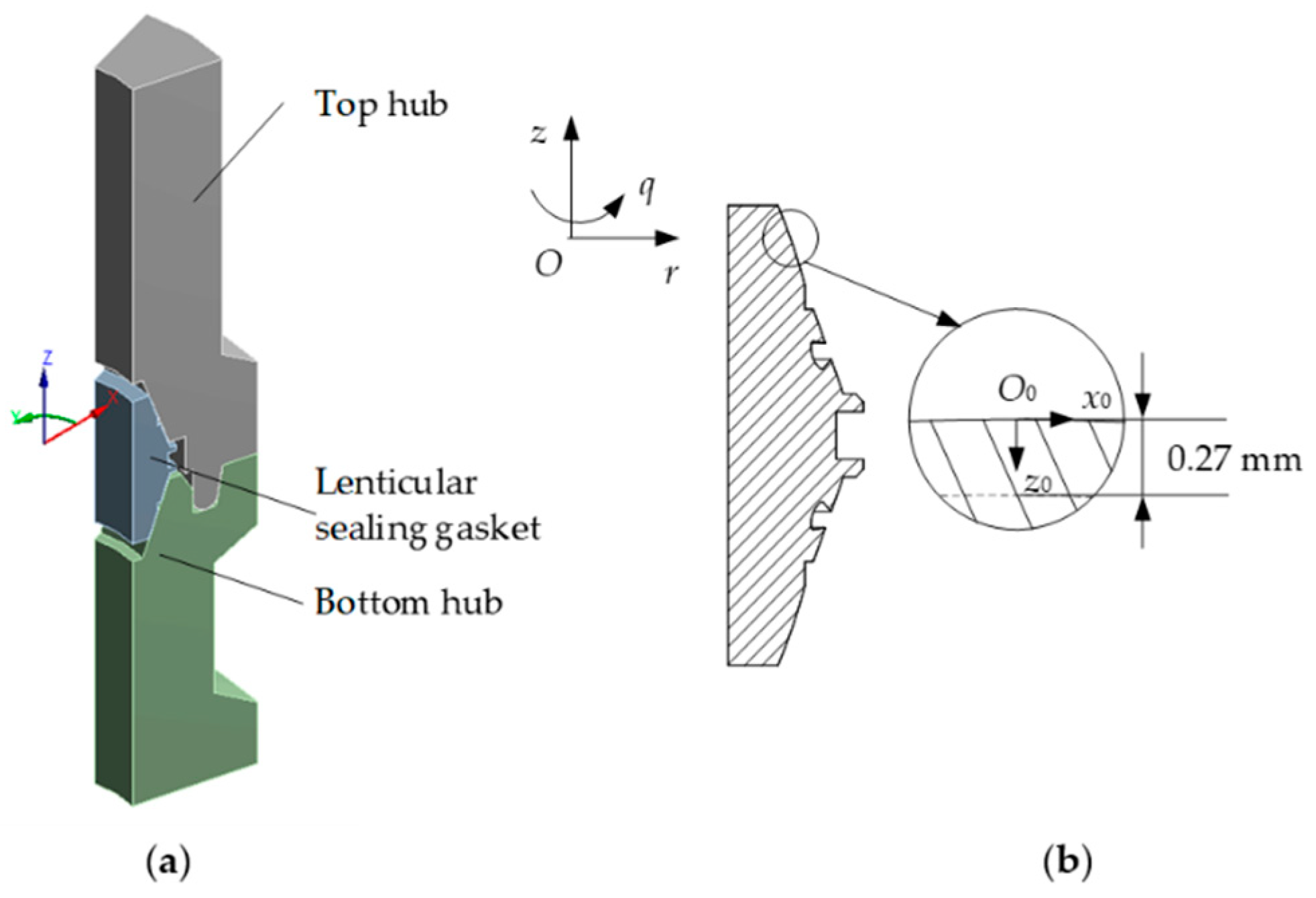
4.3.1. Contact Mechanic Analysis of the Lenticular Sealing Structure

The main sealing structure studied in this paper is the metal lenticular sealing gasket. The initial contact between the spherical surface of the lenticular sealing gasket and the conical surface of the hub is a line contact. After the connector is clamped, the contact line is further compressed and deformed into a contact belt [25,26]. However, because the contact position of the spherical surface and the conical surface is certain, the width of the contact belt is much smaller than the size of the entire sealing surface, and the width of the contact belt is also called the sealing width. In order to correctly describe the sealing performance of the lenticular sealing structure, the sealing width, contact stress mean value, and the contact stress distribution are essential key parameters. Therefore, the sealing mechanics of the lenticular sealing structure should be studied.

The contact surface between the spherical surface of the lenticular sealing gasket and the conical surface of the hub is expanded around the axis, which can be regarded as the contact between a cylinder and a plane, and it is expressed as a non-conforming surface [27] contacting the O₀ point. As shown in Figure 9, the semi-sealing width is a, the radius of the sealing sphere is r, and the elastic modulus and Poisson’s ratio of the hub and sealing gasket are E₁, E₂, μ₁ and μ₂ respectively. Therefore, the equivalent elastic modulus, E^*, can be expressed as:

$$E^{*}={\left(\frac{1-{\mu }_1^2}{E_1}+\frac{1-{\mu }_2^2}{E_2}\right)}^{-1}$$

(56)

According to Hertz contact [28], for this type of contact stress, it can be expressed as:

$$q(x_0)=\{\begin{array}{l}\frac{2P}{\pi a^2}{(a^2-x_0{}^2)}^{1/2},-a\le x_0\le a\\ 0 ,x_0<-a \& x_0>a\end{array}$$

(57)

where P is the line load, $P=(\pi E^{*}{a}^2)/4r$. Then, the maximum contact stress, q_max, is:

$$q_{\max }=q(0)=\frac{E^{*}a}{2r}$$

(58)

The mean value of contact stress, $\overline{q}$, is:

$$\overline{q}=\frac{{\displaystyle {\int }_{-a}^{a}q(x_0)d{x}_0}}{2a}=\frac{\pi E^{*}a}{8r}$$

(59)

Substituting Equation (59) into Equation (58), it can be seen that:

$$q_{\max }=\frac{4\overline{q}}{\pi }$$

(60)

Meanwhile, the semi-sealing width, a, is:

$$a=\frac{8\overline{q}r}{\pi E^{*}}$$

(61)

In the sealing width, any segment of the micro-unit is marked as ds. For the distributed force of normal contact subjected to q(s), the stress at any point (x₀,z₀) inside the sealing gasket is:

$$\{\begin{array}{l}{\sigma }_{x_0}=-\frac{2z_0}{\pi }{\displaystyle {\int }_{-a}^{+a}\frac{q(s){(x_0-s)}^{2}ds}{{[{(x_0-s)}^2+z_0{}^2]}^2}}\\ {\sigma }_{y_0}={\mu }_2({\sigma }_{x_0}+{\sigma }_{z_0})\\ {\sigma }_{z_0}=-\frac{2z_0{}^3}{\pi }{\displaystyle {\int }_{-a}^{+a}\frac{q(s)ds}{{[{(x_0-s)}^2+z_0{}^2]}^2}}\\ {\tau }_{x_0{z}_0}=-\frac{2z_0{}^2}{\pi }{\displaystyle {\int }_{-a}^{+a}\frac{q(s)(x_0-s)ds}{{[{(x_0-s)}^2+z_0{}^2]}^2}}\end{array}$$

(62)

For the contact stress distribution shown in Equation (57), on the contact interface, σ_x0 = σ_z0 = q(x₀); outside the contact area, the stress components on the surfaces of the two objects are all zero. Substituting $q(s)=\frac{2P}{\pi a^2}{(a^2-s^2)}^{1/2}$ into Equation (62) and integrating along the z₀-axis, the principal stress inside the sealing gasket in the contact area can be obtained:

$$\{\begin{array}{l}{\sigma }_{x_0}=-\frac{q_{\max }}{a}[(a^2+2z_0{}^2){(a^2+z_0{}^2)}^{-1/2}-2z_0]\\ {\sigma }_{y_0}=-\frac{2{\mu }_2{q}_{\max }}{a}[{(a^2+z_0{}^2)}^{1/2}-z_0]\\ {\sigma }_{z_0}=-q_{\max }a{(a^2+z_0{}^2)}^{-1/2}\\ {\tau }_{x_0{z}_0}=q_{\max }a[z_0-z_0{}^2{(a^2-z_0{}^2)}^{-1/2}]\end{array}$$

(63)

E. McEwen uses the variables m₀ and n₀ to express the stress at the general point [28], m₀ and n₀ can be expressed as:

$$\{\begin{array}{l}{m}_0^2=\frac{1}{2}\left({[{(a^2-x_0{}^2+z_0{}^2)}^2+4x_0{}^2{z}_0{}^2]}^{1/2}+(a^2-x_0{}^2+z_0{}^2)\right)\\ n_0^2=\frac{1}{2}\left({[{(a^2-x_0{}^2+z_0{}^2)}^2+4x_0{}^2{z}_0{}^2]}^{1/2}-(a^2-x_0{}^2+z_0{}^2)\right)\end{array}$$

(64)

where m₀ and x₀ have the same sign; n₀ and z₀ have the same sign. Thus, it can be obtained that:

$$\{\begin{array}{l}{\sigma }_{x_0}=-\frac{q_{\max }}{a}\left[m_0\left(1+\frac{z_0{}^2+n_0^2}{m_0^2+n_0^2}\right)-2z_0\right]\\ {\sigma }_{y_0}=-\frac{2{\mu }_2{q}_{\max }}{a}\left[\frac{a^2}{m_0}\left(\frac{m_0^2+n_0^2}{m_0^2-z_0{}^2}\right)-z_0\right]\\ {\sigma }_{z_0}=-\frac{q_{\max }}{a}{m}_0\left(1-\frac{z_0{}^2+n_0^2}{m_0^2+n_0^2}\right)\\ {\tau }_{x_0{z}_0}=-\frac{q_{\max }}{a}{n}_0\left(\frac{m_0^2-z_0{}^2}{m_0^2+n_0^2}\right)\end{array}$$

(65)

The contact stress of any point on the contact surface of lenticular sealing gasket and the structural stress state of any point in the contact area can be obtained in the O₀-x₀y₀z₀ coordinate system through this equation.

4.3.2. Conversion of Contact Stress

For the three-dimensional stress obtained under the action of contact stress, the main solution is the three-dimensional stress in the contact area. The structural stress of the lenticular sealing gasket is transformed into the coordinate system, and the structural stress and thermal stress caused by the internal pressure are unified under the same coordinate system. As shown in Figure 10a, the same as in Section 4.3.1, the Cartesian coordinate system O₀-x₀y₀z₀ is established with any point O₀ on the contact circle as the origin. In addition, the Cartesian coordinate system O-xyz is established with the center of the contact circle as the origin O and the axis of the sealing gasket as z-axis;d $\overrightarrow{O{O}_0}$ is the positive direction of the x-axis. Under the assumption of two-dimensional stress, the micro-body shown in Figure 10b is taken at point O₀, and the stress components σ_x0, σ_z0 and τ_x0z0 have been calculated in Section 4.3.1 of Chapter 4. Figure 10c is the orthographic projection of the micro-body. Figure 10d is the orthographic projection obtained by intercepting the micro-body with a plane parallel to Oxy, and the balance equation can be obtained:

$$\{\begin{array}{l}{\displaystyle \sum F_x}={\sigma }_{z_0}\cos \alpha \sin \alpha d{S}_0+{\tau }_{z_0{x}_0}{\sin }^2\alpha d{S}_0-{\sigma }_{x_0}\sin \alpha \cos \alpha d{S}_0-{\tau }_{x_0{z}_0}{\cos }^2\alpha d{S}_0+{\tau }_{zx}d{S}_0=0\\ {\displaystyle \sum F_z}={\sigma }_{z_0}{\sin }^2\alpha d{S}_0-{\tau }_{z_0{x}_0}\sin \alpha \cos \alpha d{S}_0+{\sigma }_{x_0}{\cos }^2\alpha d{S}_0-{\tau }_{x_0{z}_0}\cos \alpha \sin \alpha d{S}_0-{\sigma }_{z}d{S}_0=0\end{array}$$

(66)

Where ${\sigma }_{z_0}$ is the normal stress on the section of the micro-body; ${\tau }_{z_0{x}_0}$ is the shear stress on the section of the micro-body; dS₀ is the section area of the micro-body. According to the reciprocal theorem of shear stress, ${\tau }_{x_0{z}_0}$ and ${\tau }_{z_0{x}_0}$ are equal in value. Equation (66) can be written as:

$$\{\begin{array}{l}{\tau }_{zx}=\frac{{\sigma }_{x_0}-{\sigma }_{z_0}}{2}\sin 2\alpha +{\tau }_{x_0{z}_0}\cos 2\alpha \\ {\sigma }_z{=\sigma }_{x_0}{\cos }^2\alpha +{\sigma }_{z_0}{\sin }^2\alpha -{\tau }_{x_0{z}_0}\sin 2\alpha \end{array}$$

(67)

Figure 10e is the orthographic projection obtained by intercepting the micro-body with a plane parallel to Oyz. The same can be obtained:

$${\sigma }_x={\sigma }_{x_0}{\sin }^2\alpha +{\sigma }_{z_0}{\cos }^2\alpha +{\tau }_{x_0{z}_0}\sin 2\alpha$$

(68)

Substituting Equation (65) into Equation (67) and Equation (68), we can obtain:

$$\{\begin{array}{l}{\sigma }_x=\begin{array}{c}-\frac{q_{\max }}{a}\frac{n_0\left(n_0^2-z_0{}^2\right)\sin 2\alpha +\left(m_0-z_0\right)\left[m_0^2+n_0^2+\left(m_0{z}_0-n_0^2\right)\cos 2\alpha \right]}{\left(m_0^2+n_0^2\right)}\end{array}\\ {\sigma }_z=\frac{q_{\max }}{a}\begin{array}{c}\frac{n_0\left(n_0^2-z_0{}^2\right)\sin 2\alpha -\left(m_0-z_0\right)\left[m_0^2+n_0^2+\left(n_0^2-m_0{z}_0\right)\cos 2\alpha \right]}{\left(m_0^2+n_0^2\right)}\end{array}\\ {\tau }_{xz}=\frac{q_{\max }}{a}\frac{n_0\left(z_0{}^2-n_0^2\right)\cos 2\alpha +\left(m_0-z_0\right)\left(m_0{z}_0-n_0^2\right)\sin 2\alpha }{m_0^2+n_0^2}\end{array}$$

(69)

As shown in Figure 11a, the coordinate system O₀-x₀y₀z₀ is transformed by the rotation matrix ${}_o{}^{o_0}\mathrm{R}$ and the position vector ${}^{o_0}\mathrm{P}{}_o$ to obtain the coordinate system O-xyz, where:

$${}_o{}^{o_0}\mathrm{R}=\mathrm{R}(y_0,\frac{\pi }{2}+\alpha )=\left[\begin{array}{ccc}\cos (\frac{\pi }{2}+\alpha )& 0& \sin (\frac{\pi }{2}+\alpha )\\ 0& 1& 0\\ -\sin (\frac{\pi }{2}+\alpha )& 0& \cos (\frac{\pi }{2}+\alpha )\end{array}\right]=\left[\begin{array}{ccc}-\sin \alpha & 0& \cos \alpha \\ 0& 1& 0\\ -\cos \alpha & 0& -\sin \alpha \end{array}\right]$$

(70)

$${}^{o_0}\mathrm{P}{}_o={\left[\begin{array}{ccc}\frac{D_k}{2}\sin \alpha & 0& \frac{D_k}{2}\cos \alpha \end{array}\right]}^T$$

(71)

Then, the transformation relationship is:

$${}^o\mathrm{P}={}_{o_1}{}^o\mathrm{R}\hspace{0.17em}{}^{o_1}\mathrm{P}+{}^o\mathrm{P}{}_{o_1}$$

(72)

where ${}^o\mathrm{P}={\left[\begin{array}{ccc}{x}_0& y_0& z_0\end{array}\right]}^T$ is the coordinate description in O₀-x₀y₀z₀; ${}^{o_1}\mathrm{P}={\left[\begin{array}{ccc}x& y& z\end{array}\right]}^T$ is the coordinate description in O-xyz. Considering Equations (70)–(72) comprehensively, we can obtain:

$$\left[\begin{array}{c}{x}_0\\ y_0\\ z_0\end{array}\right]=\left[\begin{array}{c}\frac{D_k}{2}\sin \alpha -x\sin \alpha +z\cos \alpha \\ y\\ \frac{D_k}{2}\cos \alpha -x\cos \alpha -z\sin \alpha \end{array}\right]$$

(73)

The cylindrical coordinate system O-rθz, as shown in Figure 11b, is established at the origin of the coordinate system O-xyz, where the r-axis coincides with the x-axis. Then, according to Equation (73), it can be obtained that:

$$\{\begin{array}{l}{x}_0=\frac{D_k}{2}\sin \alpha -r\sin \alpha +z\cos \alpha \\ z_0=\frac{D_k}{2}\cos \alpha -r\cos \alpha -z\sin \alpha \end{array}$$

(74)

In the Cartesian coordinate system O-xyz and the cylindrical coordinate system O-rθz, the O₀ point has the same plane stress state, namely:

$$\left[\begin{array}{c}{\sigma }_r\\ {\sigma }_z\end{array}\right]=\left[\begin{array}{c}{\sigma }_x\\ {\sigma }_z\end{array}\right]$$

(75)

and

$${\sigma }_{\theta }={\mu }_2\left({\sigma }_r+{\sigma }_z\right)$$

(76)

From Equations (69) and (74)–(76), it can be obtained:

$$\{\begin{array}{l}{\sigma }_r^0=-a{q}_{\max }{\cos }^2\alpha \frac{1}{\sqrt{a^2+z_0{}^2}}-a{q}_{\max }\sin 2\alpha \left[z_0-\frac{z_0{}^2}{\sqrt{a^2-z_0{}^2}}\right]\\ \hspace{1em}\hspace{1em}-a^{-1}{q}_{\max }{\sin }^2\alpha \left[-2z_0+\frac{a^2+2z_0{}^2}{\sqrt{a^2+z_0{}^2}}\right]\\ {\sigma }_{\theta }^0=\frac{-2{\mu }_2{q}_{\max }}{a}\left[\sqrt{a^2+z_0{}^2}-z_0\right]\\ {\sigma }_z^0=-a{q}_{\max }{\sin }^2\alpha \frac{1}{\sqrt{a^2+z_0{}^2}}+a{q}_{\max }\sin 2\alpha \left[z_0-\frac{z_0{}^2}{\sqrt{a^2-z_0{}^2}}\right]\\ \hspace{1em}\hspace{1em}-a^{-1}{q}_{\max }{\cos }^2\alpha \left[-2z_0+\frac{a^2+2z_0{}^2}{\sqrt{a^2+z_0{}^2}}\right]\end{array}$$

(77)

where $z_0=\frac{D_k}{2}\cos \alpha -r\cos \alpha -z\sin \alpha$.

4.3.3. Thermal–Structural Coupling Stress

In order to obtain the stress caused by the combined action of multiple loads, it is necessary to couple various stresses. There are two conditions for stress superposition: one is that the system can be described as a linear second-order differential equation; the other is that the effects of various factors on the system cannot cause nonlinear phenomena [22]. The structural stress and thermal stress of the lenticular sealing gasket are both within the elastic range and can be expressed by linear second-order differential equations. With the condition for using the superposition principle, the coupling stress caused by various loads, i.e., radial stress σ_r, circumferential stress σ_θ, and axial stress σ_z, can be obtained by applying the superposition principle:

$$\{\begin{array}{l}{\sigma }_r={\sigma }_r^{\tau }+{\sigma }_r^p+{\sigma }_r^o=\frac{{\alpha }^{*}{E}_2}{1-{\mu }_2}\frac{{\tau }_i-{\tau }_o}{2\ln \left(r_o/r_i\right)}\left[-\ln \frac{r_o}{r}+\frac{r_i{}^2}{r_o{}^2-r_i{}^2}\left(\frac{r_o{}^2}{r^2}-1\right)\ln \frac{r_o}{r_i}\right]\\ \hspace{0.17em}\hspace{0.17em}\hspace{0.17em}\hspace{0.17em}+\frac{p{r}_o{}_{}^2}{r_i{}_{}^2-r_o{}_{}^2}-\frac{p{r}_i{}_{}^2{r}_o{}_{}^2}{r_i{}_{}^2-r_o{}_{}^2}\frac{1}{r^2}-a{q}_{\max }{\cos }^2\alpha \frac{1}{\sqrt{a^2+z_0{}^2}}\\ \hspace{0.17em}\hspace{0.17em}\hspace{0.17em}\hspace{0.17em}-a{q}_{\max }\sin 2\alpha \left[z_0-\frac{z_0{}^2}{\sqrt{a^2-z_0{}^2}}\right]-a^{-1}{q}_{\max }{\sin }^2\alpha \left[-2z_0+\frac{a^2+2z_0{}^2}{\sqrt{a^2+z_0{}^2}}\right]\\ {\sigma }_{\theta }={\sigma }_{\theta }^{\tau }+{\sigma }_{\theta }^p+{\sigma }_{\theta }^o=\frac{{\alpha }^{*}{E}_2}{1-{\mu }_2}\frac{{\tau }_i-{\tau }_o}{2\ln \left(r_o/r_i\right)}\left[1-\ln \frac{r_o}{r}-\frac{r_i{}^2}{r_o{}^2-r_i{}^2}\left(\frac{r_o{}^2}{r^2}+1\right)\ln \frac{r_o}{r_i}\right]\\ \hspace{0.17em}\hspace{0.17em}\hspace{0.17em}\hspace{0.17em}+\frac{p{r}_o{}_{}^2}{r_i{}_{}^2-r_o{}_{}^2}+\frac{p{r}_i{}_{}^2{r}_o{}_{}^2}{r_i{}_{}^2-r_o{}_{}^2}\frac{1}{r^2}-a{q}_{\max }{\sin }^2\alpha \frac{1}{\sqrt{a^2+z_0{}^2}}\\ \hspace{0.17em}\hspace{0.17em}\hspace{0.17em}\hspace{0.17em}+a{q}_{\max }\sin 2\alpha \left[z_0-\frac{z_0{}^2}{\sqrt{a^2-z_0{}^2}}\right]-a^{-1}{q}_{\max }{\cos }^2\alpha \left[-2z_0+\frac{a^2+2z_0{}^2}{\sqrt{a^2+z_0{}^2}}\right]\\ {\sigma }_z={\sigma }_z^{\tau }+{\sigma }_z^p+{\sigma }_z^o\hspace{0.17em}=\frac{{\alpha }^{*}{E}_2}{1-{\mu }_2}\frac{{\tau }_i-{\tau }_o}{2\ln \left(r_o/r_i\right)}\left[1-2\ln \frac{r_o}{r}-\frac{2r_i{}^2}{r_o{}^2-r_i{}^2}\ln \frac{r_o}{r_i}\right]+\frac{p{r}_o{}_{}^2}{r_i{}_{}^2-r_o{}_{}^2}-\frac{2{\mu }_2{q}_{\max }}{a}\left[\sqrt{a^2+z_0{}^2}-z_0\right]\end{array}$$

(78)

5. Numerical Simulation of Thermal–Structural Coupling of the Subsea Connector

The simulation analysis of the coupling stress of the subsea connector requires that loads such as oil and gas temperature, pre-tightening force, and oil pressure be applied to the connector, which increases the complexity of the numerical simulation. The simulation analysis model of the subsea connector is limited by constraints, with a degree of freedom of 1 and set as a 2D axisymmetric structure. The plane has 912 elements and 3165 nodes, of which the element is mainly “quad 8”. This article first carried out a numerical simulation of the temperature field of the subsea connector and then the node temperature of each component was used as a static load and was applied to the connector with the rest of the load. The thermal–structural coupling stress state of the connector under the action of the steady-state temperature field was obtained by statics. In the simulation, F22 material was used for hubs and fingers, and Incoloy 825 nickel-chromium iron corrosion resistant alloy material was selected for the sealing gasket.

5.1. Steady-State Temperature Field Analysis of the Subsea Connector

Under rated working conditions, the subsea connector has high-temperature oil and gas flowing inside and is exposed to low-temperature seawater outside. Set the surface temperature of hub and lenticular sealing gasket in contact with oil and gas to be 150 °C and seawater temperature to be 3 °C. For the surface exposed to the seawater environment, the equivalent thermal conductivity and composite heat transfer coefficient obtained from Section 3 are used according to the third boundary condition.

5.2. The Overall Temperature Field Distribution of the Connector Sealing Structure

Figure 12 shows the overall steady-state temperature field of the subsea connector sealing structure. It can be seen that the overall temperature distribution of the connector gradually decreases from the inside to the outside. The temperature of the top and bottom hub and the inner wall of the lenticular sealing gasket is relatively high, which is above 143.39 °C. The maximum temperature of the system is 150 °C, which is on the innermost side of the lenticular sealing gasket and hub. The temperatures of the finger and the press ring are low, the temperature of the main body of the finger is below 61.506 °C, the temperature of the main body of the press ring is below 14.566 °C, and the lowest temperature of the system is 3.0697 °C at the end of the finger.

The lenticular sealing gasket is in direct contact with high-temperature oil and gas and is located inside of the connector leading to low heat emission efficiency and concentrated heat, so the temperature is the highest. Although the hub is in direct contact with high-temperature oil and gas, the outer wall of the hub is directly exposed to low-temperature seawater, so the heat emission efficiency of the hub is higher than that of the lenticular sealing gasket. Most of the surroundings of the finger are in low-temperature seawater. Since the finger temperature is relatively high, the tail is far from the main body and is not in contact with the hub and lenticular sealing gasket of higher temperature, so the temperature is the lowest.

In order to show the temperature gradient inside the connector more intuitively, as shown in Figure 13a, a path from the midpoint P_i of the lenticular sealing gasket to the point P_o on the outer surface of the press ring is established. The temperature change of each point on the path is shown in Figure 13b. Among the components of the subsea connector, the temperature of the lenticular sealing gasket drops by 22.32 °C, and the temperature gradient is −0.79 °C/mm; the temperature of the hub drops by 60.01 °C, and the temperature gradient is −1.05 °C/mm; the temperature of the finger drops by 19.54 °C, and the temperature gradient is −0.38°C/mm; the temperature of the press ring drops by 2.64 °C, and the temperature gradient is −0.03 °C/mm. In the seawater layer, the temperature of the seawater layer 1 between the sealing gasket and the hub drops by 9.32 °C, and the temperature gradient is −1.33 °C/mm; the temperature of the seawater layer 2 between the flange and the finger drops by 4.63 °C, and the temperature gradient is −1.16 °C/mm; the temperature of the seawater layer 3 between the finger and the press ring drops by 5.07 °C, and the temperature gradient is −0.60 °C/mm.

It can be seen that on the path P_iP_o, the falling temperature and temperature gradient of the hub are the maximum values of all parts, and the values of the sealing gasket, finger, and press ring decrease in order, which is consistent with the previous analysis.

Temperature Field Distribution of the Lenticular Sealing Gasket

Since the lenticular sealing gasket is the easiest to use to conduct a comparative analysis between theory and simulation in the subsequent thermal–structural coupling process, its steady-state temperature field is discussed separately here. The temperature distribution of the lenticular sealing gasket is shown in Figure 14a. The temperature is uniformly distributed along the circumferential direction and gradually decreases from the inside to the outside and the temperature gradient is small. The highest temperature is 150 °C, which is generated on the inner wall and at the end of the lenticular sealing gasket; the lowest temperature is 126.46 °C, which is generated in contact with the seawater layer. As shown in Figure 14b, a path is established from the upper end face to the lower end face. The temperature on the extraction path is shown in Figure 14c, which clearly shows that the temperatures of the upper and lower parts of the lenticular sealing gasket are approximately symmetrically distributed. On this path, from 0~27.5 mm, the temperature continuously decreases from 150 °C to 142.68 °C; from 27.5~65 mm, the temperature slowly rises to 145.32 °C; from 65~92.5 mm, the temperature slowly drops again to 144.22 °C; from 92.5~118 mm, the temperature quickly rises to 150 °C.

The overall temperature of the lenticular sealing gasket exceeds 126 °C, so there is no need to worry about large internal stress changes due to an excessive temperature gradient. At the same time, Incoloy 825 has good high-temperature mechanical properties, and the temperature between 126~150 °C has little effect on its mechanical properties. It can be seen that the lenticular sealing gasket can maintain good sealing performance under the steady-state temperature distribution.

5.3. Analysis of Coupling Stress Examples under a Steady-State Temperature Field

The stress analysis of the lenticular sealing gasket of the subsea connector under the combined action of preload, internal pressure, and temperature load is carried out by using the composite stress expression of steady-state thermal structural coupling analyzed in Section 4.3.3, and the results are compared with the finite element simulation results.

The coupling stress analysis model of the lenticular sealing gasket is shown in Figure 15a, and this analysis was carried out by using the core sealing structure of the 1/12 subsea connector.

Table 1. Coupling stress calculation parameters.

Parts	Material Parameter					Boundary Conditions
	E(MPa)	ν	ρ (g/cm3)	λk (W∙m−1∙K−1)	α* (/°C)	qmax (MPa)	P (MPa)	τ (°C)
Gasket	2.06 × 105	0.25	7.93	16.7	1.70 × 10−5	458.03	34.5	10.17
Hubs	2.1 × 105	0.3	7.93	16.3	1.68 × 10−5

shows the material parameters of each part. The inner side of the structure is subjected to an internal pressure of 34.5 MPa. Frictionless support is used on both sides of the radial direction. The bottom of the bottom hub is set as the fixed end, and 1/12 of the axial pre-tightening force [29], which is 856.8 kN, is applied to the top of the top hub. At the same time, the steady-state temperature field analysis results of 150 °C inside and 3 °C outside the connector are introduced to simulate the thermal–structural coupling stress of the connector, and the sealing characteristics of the lenticular sealing gasket under the thermal–structural coupling action are obtained. The finite element simulation analysis in the previous section shows that the temperature difference between the inside and outside of the lenticular sealing gasket is τ = 10.17 °C, and the initial maximum contact stress is q_max = 458.03 MPa. These and other parameters are recorded in Table 1.

As shown in Figure 15b, in order to study the sealing performance of the lenticular sealing gasket under the action of thermal–structural coupling, the contact position of the lenticular sealing gasket on any side can be used for analysis. From the analysis in Section 4.3.1, it can be seen that on the contact interface of the seal gasket, the principal stress is the contact stress, which cannot be superimposed with the structure thermal stress in Section 4.1. In the contact area of the sealing gasket, after the stress coordinate transformation in Section 4.3.2, the stress at any point has been given by Equation (77), which is the same as the calculation method of structure thermal stress, so thermal–structural coupling can be carried out. As shown in Figure 15b, in order to facilitate the finite element simulation analysis, the connecting line between the two endpoints on both sides of the sealing surface is taken as the analysis position, and the distance between the connecting line and the contact surface is 0.27 mm.

Substituting the known parameters into Equation (78), the theoretical calculation results of the three-dimensional stress in the cylindrical coordinate system are obtained, and the comparison with the results obtained by the simulation analysis is shown in Figure 16. The change trend of the three-dimensional stress in the sealing width of the theoretical analysis is basically the same as the simulation result. Since the lenticular sealing gasket is under pressure, the three-dimensional stress is negative. As shown in Figure 16a, the theoretical maximum value of radial stress σ_r along the negative direction of r-axis is 477.94 MPa, and the simulation maximum value is 453.95 MPa, both of which occur at the contact center. The theoretical analysis is 5.28% higher than the simulation analysis. As shown in Figure 16b, the maximum value of circumferential stress σ_θ occurs at the contact center. Along the negative direction of the θ-axis, the theoretical maximum value is 91.17 MPa, and the simulation maximum value is 83.78 MPa. The theoretical analysis is 8.82% larger than the simulation analysis. As shown in Figure 16c, the maximum value of the axial stress σ_z also occurs at the contact center. Along the negative direction of the z-axis, the theoretical maximum value is 344.08 MPa, and the simulation maximum value is 326.71 MPa. The theoretical analysis is 5.32% larger than the simulation analysis. At the same time, Figure 16 shows that at z₀ = 0.27 mm, the sealing width of theoretical analysis is about 5.52 mm, and the sealing width of simulation analysis is about 6.28 mm. The theoretical analysis is 12.10% lower than the simulation analysis. The absolute values of the stress of σ_θ and σ_z on the negative semi-axis of the x-axis are less than those on the positive semi-axis of the x-axis.

After analysis, it can be seen that the theoretical coupling stress analysis first performs the two-dimensional stress analysis and then performs the three-dimensional expansion, while the simulation directly performs three-dimensional finite element analysis. There is a certain algorithm error between the two. Since the two contact surfaces are assumed to be smooth in the theoretical analysis, the edge position of the sealing width is greatly affected. At the same time, due to the influence of friction, the stress at the bottom end of the contact position of the sealing gasket is greater than that at the top end, and σ_θ and σ_z are the most obvious stresses affected by this influence.

5.4. Coupling Stress Analysis in the Pressure Shock Mode

The pressure shock mainly simulates that the connector is subjected to a shock higher than the working pressure in a short time when the temperature is stable. As shown in Figure 17, the shock pressure used is 1.5 times of the rated working pressure (51.75 MPa). Figure 18 shows the change of the maximum contact stress of the lenticular sealing gasket and the maximum equivalent stress of each component. As shown in

Table 2. Contact stress and equivalent stress of the main sealing structures in every stage in the pressure shock mode.

Time (s)	Maximum Contact Stress (MPa)	Maximum Equivalent Stress (MPa)
		Lenticular Sealing Gasket	Hub	Finger
10	458.76	251.85	176.64	111.79
20	492.59	275.22	195.21	113.00
30	459.06	251.88	176.99	111.87
40	458.76	251.85	176.64	111.87

, the parameters under this working condition are extracted.

After analysis, it can be seen that the change trend of the maximum contact stress of the lenticular sealing gasket with the pressure shock is similar to that under the condition of rapid pressure rise and pressure reduction. Under the steady-state temperature distribution, when the oil gas pressure load reaches 1.5 times of the rated working pressure, the maximum contact stress of the lenticular sealing gasket increases from 458.76 MPa to 492.59 MPa, which meets the contact stress conditions of the oil and gas sealing. Under the impact load of oil and gas pressure, the maximum equivalent stress of the finger is 113.00 MPa, and the maximum equivalent stress of the hub is 195.21 MPa, both of which are below the theoretical yield limit (310 MPa) of the 12Cr2Mo1 material. At the same time, the change of the maximum equivalent stress of the finger is 1.21 MPa, and the change of the maximum equivalent stress of the hub is 18.57 MPa, which shows that the finger is affected by a smaller impact. The maximum equivalent stress at the spherical surface of the lenticular sealing gasket is 275.22 MPa, which is 23.37 MPa higher than the rated working pressure, and this stress further aggravates the elastoplastic and plastic deformation of the sealing spherical surface. It shows that the lenticular sealing gasket is more sensitive to high pressure under high temperature conditions and is prone to produce large plastic deformation. During the service period of the connector, it is necessary to avoid opening and closing the wellhead several times in a short time, so as to prevent the connector from pressure impact and fatigue wear on the sealing surface under high temperature.

6. Conclusions

In this article, the heat transfer model of the subsea connector is established and solved, and the steady-state temperature distribution of the connector is obtained. Considering the stress and deformation of the subsea connector under the thermal load, the thermal–structural coupling analysis model of steady-state temperature field is established. The theoretical analysis of thermal stress of the key sealing structures of the connector is compared with the numerical simulation, and the pressure shock mode under the steady-state temperature field is also analyzed. It is proved that the coupling mathematical model proposed in this article can be applied to the thermal–structural coupling theoretical analysis of the similar subsea oil and gas equipment. The main conclusions are as follows:

(1)

Considering the heat transfer problem of the subsea connector in deep water, the equivalent heat transfer models of seawater layer between the lenticular sealing gasket and hubs, between hubs and fingers, and outside the outer surface of the fingers and the press ring are established, and the relationship between equivalent thermal conductivity, composite heat transfer coefficient, and temperature is solved.

(2)

The mathematical model of steady-state thermal structural coupling of the subsea connector is established and verified by the simulation analysis. The theoretical analysis of the radial stress, circumferential stress, and axial stress is 5.28%, 8.82%, and 5.32% larger than the simulation analysis, and the sealing width is 12.10% smaller.

(3)

The steady-state temperature distribution of the subsea connector under rated working condition is simulated. The finite element simulation shows that in the center path of the connector’s lenticular sealing gasket, the hub’s falling temperature is 60.01 °C and the temperature gradient is −1.05 °C/mm, which are the maximum values of all parts. The values of the sealing gasket, finger, and press ring decrease in turn. The temperature field of the lenticular sealing gasket is symmetrically distributed, and the temperature is always in the high temperature stage (126~150 °C), which has little influence on the mechanical properties of the material, so as to ensure its stable sealing performance.

(4)

The numerical simulation of pressure shock mode under steady temperature field shows that the maximum equivalent stress of the sealing gasket exceeds the theoretical yield limit of the material under the combined action of temperature and pressure, resulting in plastic deformation, which indicates that the lenticular sealing gasket is sensitive to high pressure shock under high temperature.

References

1. Bai, Y.; Bai, Q. Subsea Pipelines and Risers, 1st ed.; Elsevier Science Ltd.: Kidlington, UK, 2005; pp. 3–19. [Google Scholar]
2. Toshiyuki, S.; Wataru, M. Thermal Stress Analysis and Sealing Performance Evaluation of Pipe Flange Connections with Spiral Wound Gaskets under Elevated Temperature. In Proceedings of the ASME Pressure Vessels and Piping Conference, San Diego, CA, USA, 25–29 July 2004. [Google Scholar]
3. Abid, M.; Ullah, B. Three-Dimensional Nonlinear Finite-Element Analysis of Gasketed Flange Joint under Combined Internal Pressure and Variable Temperatures. J. Eng. Mech. 2007, 133, 222–229. [Google Scholar] [CrossRef]
4. Zhou, X.; Chou, X.; Zhang, B.; Chen, G. Finite Element Analysis of Bolt-Connected Flange Transient Temperature Field. Press. Vess. T 2007, 24, 8–11, 16. [Google Scholar]
5. Al-Turki, L.I.; Drummond, J.L.; Agojci, M.; Gosz, M.; Tyrus, J.M.; Lin, L. Contact versus flexure fatigue of a fiber-filled composite. Dent. Mater. 2007, 23, 648–653. [Google Scholar] [CrossRef] [PubMed]
6. Avanzini, A.; Donzella, G. A computational procedure for life assessment of UHP reciprocating seals with reference to fatigue and leakage. Int. J. Mater. Prod. Technol. 2007, 30, 33. [Google Scholar] [CrossRef]
7. Omiya, Y.; Sawa, T. Thermal Stress Analysis and the Sealing Performance Evaluation of Bolted Flange Connection at Elevated Temperature. In Proceedings of the ASME 2009 Pressure Vessels and Piping Conference, Prague, Czech Republic, 26–30 July 2009. [Google Scholar]
8. Toshiyuki, S.; Yoshio, T.; Hiroyasu, T. Effect of Material Properties of Gasket on the Sealing Performance of Pipe Flange Connections at Elevated Temperature. In Proceedings of the ASME 2015 Pressure Vessels and Piping Conference, Boston, MA, USA, 19–23 July 2015. [Google Scholar]
9. Luo, Y.; Liu, X.; Hao, J.; Wang, Z.; Liu, L.; Lin, X. Research on thermal fatigue failure mechanism of aviation electrical connectors. Acta Armamentarii 2016, 7, 1266–1274. [Google Scholar]
10. Wang, L.; Chen, X.; Fan, Z.; Xue, J. FEM Stress Analysis of Bolted Flange Joints in Elevated Temperature Service Condition. In Proceedings of the ASME 2018 Pressure Vessels and Piping Conference, Prague, Czech Republic, 15–20 July 2018. [Google Scholar]
11. Abdullah, O.I.; Schlattmann, J.; Jobair, H.; Beliardouh, N.E.; Kaleli, H. Thermal stress analysis of dry friction clutches. Ind. Lubr. Tribol. 2018, 72, 189–194. [Google Scholar] [CrossRef]
12. Lanzhu, Z.; Guangkai, X. Analysis of the metal-to-metal contact flange joint subject to external bending moment. Proc. Inst. Mech. Eng. Part E J. Process Mech. Eng. 2018, 233, 234–241. [Google Scholar]
13. Tang, L.; He, W.; Zhu, X.; Zhou, Y. Sealing Performance Analysis of an End Fitting for Marine Unbonded Flexible Pipes Based on Hydraulic-Thermal Finite Element Modeling. Energies 2019, 12, 2198. [Google Scholar] [CrossRef] [Green Version]
14. Chen, J.; Ding, X.; Zhang, W.; Yan, R.; Sun, B. Fractal prediction model for the thermo-elastic normal contact stiffness of frictional interfaces in dry gas seals. J. Vib. Shock. 2020, 39, 257–263. [Google Scholar]
15. Wang, Q.; Hu, Y.P.; Ji, H.H. Leakage, heat transfer and thermal deformation analysis method for contacting finger seals based on coupled porous media and real structure models. Proc. Inst. Mech. Eng. Part C J. Mech. Eng. Sci. 2020, 234, 2077–2093. [Google Scholar] [CrossRef]
16. Fukuoka, T.; Yao, Y. Evaluation of Thermal and Mechanical Behaviors of Pipe Flange Connections for Low Temperature Fluids by Numerical Analysis and Experiments. Mar. Eng. 2015, 50, 671–677. [Google Scholar] [CrossRef] [Green Version]
17. Tsuta, T.; Yamaji, S. Boundary element analysis of contact thermo-elastoplastic problems with creep and the numerical technique. In Proceedings of the 5th BEM Conference, Hiroshima, Japan, 8–11 November 1983; p. 576. [Google Scholar]
18. Sharqawy, M.H. New correlations for seawater and pure water thermal conductivity at different temperatures and salinities. Desalination 2013, 313, 97–104. [Google Scholar] [CrossRef]
19. Kretzschmar, H.; Cooper, J.R.; Dittmann, A.; Friend, D.G.; Gallagher, J.S.; Harvey, A.H.; Knobloch, K.; Mareš, R.; Miyagawa, K.; Okita, N.; et al. Supplementary Release on Backward Equations for the Functions T(p,h), v(p,h) and T(p,s), v(p,s) for Region 3 of the IAPWS Industrial Formulation 1997 for the Thermodynamic Properties of Water and Steam. J. Eng. Gas Turbines Power 2007, 129, 294–303. [Google Scholar] [CrossRef]
20. Cooper, J.R.; Dooley, R.B. Revised Release on the IAPWS Industrial Formulation 1997 for the Thermodynamic Properties of Water and Steam. In Proceedings of the International Association for the Properties of Water and Steam, Lucerne, Switzerland, 26–31 August 2007; pp. 1–49. [Google Scholar]
21. Abid, M.; Khan, K.A.; Chattha, J.A. Performance of a Flange Joint using Different Gaskets under Combined Internal Pressure and Thermal Loading, a FEM Approach. Mech. Based Des. Struct. Mach. 2008, 36, 212–223. [Google Scholar] [CrossRef]
22. Cheng, X.; Peng, W.; Sun, L.; Li, X.; Yin, Z. Analysis of the fracture pattern and failure time of LNG outer tanks under the action of thermal load. Nat. Gas Ind. 2015, 35, 103–109. [Google Scholar]
23. Hetnarski, R.B. Encyclopedia of Thermal Stresses; Springer: Dordrecht, The Netherlands, 2014; pp. 1241–1522. [Google Scholar]
24. Lu, G.C.; Chu, G.N. Research of Directional Stress Distribution on the Fully Plastic Bulged Pressure Hull. Adv. Mater. Res. 2014, 1082, 412–415. [Google Scholar] [CrossRef]
25. Yang, Y.; Zhu, H.; He, D.; Du, C.; Xu, L.; He, Y.; Zheng, Y.; Ye, Z. Contact mechanical behaviors of radial metal seal for the interval control valve in intelligent well: Modeling and theoretical study. Energy Sci. Eng. 2019, 8, 1337–1352. [Google Scholar] [CrossRef]
26. Li, Y.; Zhao, H.; Wang, D.; Xu, Y. Metal sealing mechanism and experimental study of the subsea wellhead connector. J. Braz. Soc. Mech. Sci. Eng. 2019, 42, 26. [Google Scholar] [CrossRef]
27. Polycarpou, A.A.; Etsion, I. A Model for the Static Sealing Performance of Compliant Metallic Gas Seals Including Surface Roughness and Rarefaction Effects. Tribol. Trans. 2000, 43, 237–244. [Google Scholar] [CrossRef]
28. Johnson, K. Contact Mechanics; Cambridge University Press: Cambridge, UK, 1987; pp. 12–119, 451–481. [Google Scholar]
29. Yun, F.; Wang, L.; Yao, S.; Liu, J.; Liu, T.; Wang, R. Analytical and experimental study on sealing contact characteristics of subsea collet connectors. Adv. Mech. Eng. 2017, 9, 168781401770170. [Google Scholar] [CrossRef] [Green Version]
Figure 1. The subsea connector. (a) Installation tool and top connector; (b) the structure of the subsea connector.
Applsci 12 03194 g001
Figure 2. Heat transfer model of the subsea collet connector.
Applsci 12 03194 g002
Figure 3. Heat transfer of the seawater between the hub and collet.
Applsci 12 03194 g003
Figure 4. Relationship between λe1 and the temperature.
Applsci 12 03194 g004
Figure 5. Heat transfer between the hub and the lenticular sealing gasket. (a) Schematic diagram of heat transfer; (b) Simple diagram of heat transfer.
Applsci 12 03194 g005
Figure 6. Relationship between λe2 and the temperature.
Applsci 12 03194 g006
Figure 7. Heat transfer of the collet outer surface and the press ring outer surface.
Applsci 12 03194 g007
Figure 8. Relationship between the composite thermal conductivity he and the temperature.
Applsci 12 03194 g008
Figure 9. Contact principle diagram of the seal gasket.
Applsci 12 03194 g009
Figure 10. Stress state analysis near the contact position. (a) The contact position; (b) The micro-body; (c) Orthographic projection of the micro-body; (d) The orthographic projection obtained by intercepting the micro-body with a plane parallel to Oxy; (e) The orthographic projection obtained by intercepting the micro-body with a plane parallel to Oyz.
Applsci 12 03194 g010
Figure 11. Coordinate transformation. (a) Coordinate system transformed; (b) The cylindrical coordinate system.
Applsci 12 03194 g011
Figure 12. Steady-state temperature field of the whole subsea collet connector.
Applsci 12 03194 g012
Figure 13. Steady-state temperature distribution of the subsea collet connector on the center path. (a) Temperature path PiPo; (b) The temperature change at each point along the path PiPo.
Applsci 12 03194 g013
Figure 14. Steady-state temperature field of the lens seal gasket. (a) Temperature field nephogram; (b) Path of the temperature field; (c) Temperature distribution along the path.
Applsci 12 03194 g014
Figure 15. Simulation and calculation model of the sealing structure. (a) Simulation model; (b) Location of stress calculation.
Applsci 12 03194 g015
Figure 16. Stress distribution in the sealing width when z0 is 0.27 mm. (a) Distribution of σr at z0 = 0.27 mm; (b) Distribution of σθ at z0 = 0.27 mm; (c) Distribution of σz at z0 = 0.27 mm.
Applsci 12 03194 g016
Figure 17. Pressure shock mode.
Applsci 12 03194 g017
Figure 18. Maximum contact stress and equivalent stress changing with the oil and gas pressure in the pressure shock mode. (a) Maximum contact stress; (b) Maximum equivalent stress.
Applsci 12 03194 g018