Abstract
During an earthquake, seismic waves travel through different media through the source to reach the surface. It is very necessary to study the dynamic characteristics of soil between different layers during earthquake. In order to explore the dynamic characteristics of soil under the action of ground seismic input motion, scaled-down model tests were carried out through 1 g shaking table tests based on a laminar shear box. After creating a dense lower ground with a sample of mixed silica and silty soil, and a loose upper ground with sand, the acceleration was measured by applying seismic loading through the 1 g shaking table test. Through the Peak ground acceleration, Spectral acceleration and Spectral acceleration amplification factors, the magnification variation and differences of each depth of the model and the dynamic characteristics of soil between different layers were displayed. In order to verify the reliability of the experimental data, a one-dimensional ground response analysis was carried out using DEEPSOIL software. The approximate results obtained by comparing each other can provide a basis for the accuracy of the experimental results.
1. Introduction
Multilayered ground consists of two or more layers with different material properties, stratum density and shear wave velocity. Ground amplification is caused by differences in impedance at each layer. Therefore, the amplification characteristics of the ground are determined by the differences in the physical properties of each layer that constitutes the ground. In order to confirm this through model tests, a multilayered ground model was created and to observe changes in the behavior and amplification characteristics between layers under seismic loading. To this end, two or more different materials forming a multilayered ground were used to identify each property, and test methods suitable for multilayered ground were explored and carried out.
In order to understand the complex ground behavior during earthquakes, several experimental studies have been carried out using the 1 g shaking table test. However, most of the studies were systematically performed by changing the ground conditions such as soil material, density (water content), inclination angle of the slope, and ground water level [1]. Shinoda et al. [2] produced bedrock using well-graded gravel, cement, and water at a weight ratio of 90.1%:3.6%:6.3%; the dynamic strain during shaking was successfully measured to understand the generation of shear strain. Yang [3] studied the influence of pore water saturation on the horizontal and vertical components of ground motion in multi-layer soil bedrock system under the action of inclined SV wave. Only a few studies have proposed the characteristics of the input motion, in which the peak ground acceleration is also the main focus, just few studies have focused on the frequency characteristics [1]. Wartman et al. [4] compared the relationship between the dominant frequency of the input ground motion and the natural frequency. Brennan and Madabhushi [5] showed that the acceleration amplification rate is different between the center and edge of the crest using the centrifugal model tests. Abe et al. [6] conducted a numerical study of the dynamic behavior from deformation to failure of a slope model (including various inclined weak layers) using shaking table tests. Hou et al. [7] studied the stability of a nonhomogeneous slope with cracks under earthquake action. The failure mechanism of a nonuniform slope with cracks was proposed for the first time using the discretization technique. According to the obtained numerical and laboratory test results, Goktepe et al. [8] concluded that the carefully selected large geometric-scale coefficients for the soil-structure model used in the small-scale shaking table experiments can capture the dynamic response of the full-scale soil-structure system with acceptable accuracy. Song et al. [9] studied the influence of natural frequency on slope dynamic characteristics. Numerical and experimental results show that the high frequency component and low frequency component mainly cause local deformation and whole deformation of the surface slope respectively. Zhang et al. [10] introduced shaking table tests to resolve the response differences between underground shafts and tunnels during earthquakes, to evaluate their impact on structural performance, and to verify the proposed model by comparing test and analysis results. Nakamura [11] used the 1 g shaking table test to analyze slope instability. The slope model consists of three layers: surface layer, weak layer and base layer. The applicability of the Newmark method is verified.
As we know, foundations are made up of many grounds of soil. It is very difficult to capture the dynamic characteristics of soil during an earthquake at a real site. Usually, it is difficult to create actual natural rock, and it is common to imitate the bedrock by mixing sand, cement, or silica due to the high risk of failure. However, due to the possibility of damage to equipment in constructing bedrock and the difficulty in laying and removing accelerometers, it is recommended to change the compaction level of the soil to form the ground, or to create a multilayered ground by mixing gravel and collected soil samples. Thus, it is necessary to utilize materials with different properties and densities to implement more than one layer with different ground properties. Although there are many studies using numerical analysis, most of the analyses have been performed to study a single type of soil, which is not consistent with the actual situation. Furthermore, many studies consider boundary effects but ignore variations and differences in seismic wave amplification through the ground with two different soil properties. In this paper, the dynamic characteristics of multilayered ground under the different seismic waves were analyzed by using the 1 g shaking table test. By creating multilayered ground, different layers have different natural frequencies. Due to the differences in physical properties between layers and the existence of a boundary between layers, the amplification characteristics and dynamic performance differences of each layer can be clearly captured. Combined with the experimental method and analysis method, the dynamic characteristics of various grounds can be explored. Shaking table tests are performed by creating a multilayered ground and verified by numerical analysis, which was not very common in previous studies. This way combined with the similarity law, the dynamic behavior of large-scale models can be easily predicted. Based on previous studies, this study considers in more detail the problems that will be faced in the actual ground.
2. Materials and Methods
2.1. Soil Properties and Experimental Equipment
The soil used in the model test was collected from a cut slope at a construction site in Ulju-gun, Ulsan Metropolitan City to represent the domestic reclamation and weathered soil slopes. To analyze the geotechnical index properties of the sample, the specific gravity test, the particle size analysis test and the standard proctor test were performed. According to the analysis of the grain size distribution curve, the finer content of the sample was 10.8%. The specific gravity of the soil was 2.69 and the optimum moisture content of the soil was 12.5%. The maximum dry weight was 18.29 kN/m3, and the minimum dry weight was 12.43kN/m3. The Atterberg limit test showed Non-Plastic (NP) for the Plastic Index (PI). The elastic modulus calculated by shear wave velocity was 2 × 10⁷ Pa. The sample corresponds to SW-SM when classified under the Unified Soil Classification System (USCS). The maximum void ratio was 1.123 and the minimum void ratio was 0.443. The Internal Friction Angle was 27.7°, and the Dilatancy angle was 24.4°. Table 1 summarizes the test results for the basic physical properties of loose ground.

Table 1.
Geotechnical index properties of the specimen (loose ground) used in this study (Jin et al. [12]).
In order to create a layered ground of a flat model with two different ground properties, the dense ground was created by mixing soil and silica sand with a diameter of 2–5 mm in a weight ratio of 6:4. The unit weight of the combined sample was 21.5 kN/m3. For the loose ground sample, the specific gravity test, the particle size analysis test and the standard proctor test were carried out. Since it is mixed soil, Table 2 lists the physical properties required for the experiment. According to the analysis of the grain size distribution curve, the finer content of the sample was 6.48%. The specific gravity of the soil was 2.63, the optimum moisture content of the soil was 8.14%. The maximum void ratio was 0.923, and the minimum void ratio was 0.487. The maximum dry weight was 18.95 kN/m3, and the minimum dry weight was 14.65 kN/m3.
Table 2.
Geotechnical index properties of the specimen (dense ground) used in this study.
Figure 1 is the conceptual diagram of the structure and shaking table test equipment used in this experiment.
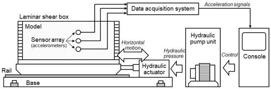
Figure 1.
The experimental system used in this study (Kim et al. [13]).
In this study, a number of frames that are freely operated in the horizontal direction are composed of soft elements capable of mimicking infinitely extended ground boundary conditions for horizontal shear motion. This flexible structure has dimensions of 200 cm (width) × 60 cm (length) × 60 cm (height) and consists of 12 layers of aluminum frames. Each frame is 4.5 cm thick and the spacing between frames is about 0.5 cm. Each frame can move independently of each other in horizontal directions through roller bearings. The natural periods of the empty box and fill box are 0.04~0.05 s and 0.1 s. Figure 2 shows the empty Laminar shear box and soil sample set up in the box.
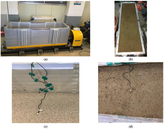
Figure 2.
Laminar shear box: (a) Empty Laminar shear box in this study; (b) Soil sample set up in the LSB; (c) Accelerometer set up for a dense layer; (d) Accelerometer set up for a loose layer.
When using a 1 g shaking table for dynamic testing, it is very important to select accelerometers and a data logger suitable for test purposes. Figure 3 shows the data logger and accelerometer used in this study. The prediction range of response acceleration measured in this test is no more than 20 m/s2, the frequency component of response data is 40 Hz, and the temperature is room temperature. Therefore, an ARF-20A acceleration transducer, which can be measured up to 20 m/s2, was selected for the accelerometer. The mass of the accelerometer should be less than or equal to the ground density so as not to affect the inertia of the accelerometer. The weight of the test accelerometer is 13 g. The data logger has 24 channels, compatibles with the ARF-20A, the data heap itself features L.P filter, and the data storage interval is up to 0.005 s. The main parameters of accelerometers and data logger are shown in Table 3.
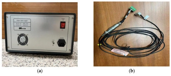
Figure 3.
Acceleration capture instrument in this study: (a) Data logger; (b) Accelerometer.
Table 3.
Main parameters of accelerometer and data logger.
2.2. Model Construction and Experimental Procedures
In this study, the amplification characteristics of acceleration have been investigated for the flat ground model with multilayered soils. The cross-section and accelerometer location of the model ground created in this experiment are illustrated in Figure 4. The two layers consisted of loose and dense ground, respectively, and the height of each layer was 0.3 m. The upper ground was formed relatively loosely with a unit weight of 14.72 kN/m3 using sampling soils, and the lower ground was densely formed with a unit weight of 19.6 kN/m3 using mixing samples. In order to confirm the change in the amplification characteristics between the two layers, accelerometers were buried 5 cm apart from the ground floor to the surface at the center, which was considered to best simulate the free field behavior. However, if the accelerometer is buried on only one axis at an interval of 5 cm, the gap between the instruments is too short to disturb the ground or measure distorted signals. Therefore, it was alternately buried on two axes, 5 cm away from the center axis and center axis.
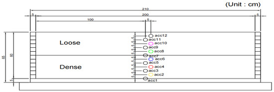
Figure 4.
The cross-section and accelerometer location of the flat ground.
The input seismic wave was selected from the sine wave, sine sweep wave, and artificial seismic wave. As sine wave signals, the 10 Hz signals corresponding to the Peak ground acceleration of 0.2 g were used to confirm the basic characteristics of the flat model. A simple long-period sine 10 Hz wave was chosen so that resonance would not occur due to the natural period of the shaking table or box. The artificial seismic wave is a composite seismic wave combined with the Gyeongju-Pohang earthquake, using the empirical Green’s function based on raw data measured at the Kori nuclear power plant. Since artificial seismic waves have different periodic components, high amplification occurs. There is also a sine sweep wave that provides waves containing any frequency from low to high frequencies. Seismic motion includes waves of various frequency bands from low to high frequencies. They are used to determine amplification characteristics that resonate with the natural frequencies of the ground. The acceleration-time history of the input seismic wave shaking table test above is shown in Figure 5.
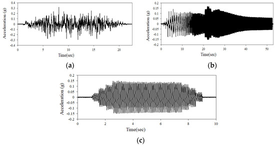
Figure 5.
Time-histories of the input ground motions used in this study: (a) artificial earthquake wave; (b) sine sweep wave; (c) sine 10 Hz wave.
3. Multilayered Flat Model Ground Test Results and Analysis
3.1. Shear Wave Velocity
The shear wave velocity is usually used to characterize the dynamic property of soil in geotechnical engineering, and the importance of shear wave velocity in geotechnical seismic engineering has been widely recognized and applied in seismic design and seismic performance evaluation [14]. The average shear wave velocity of the model was obtained by substituting the difference between the distance between the two accelerometers buried in the ground and the arrival time of the shock wave into the velocity formula by giving an impact to the lower part of the soil box in Equation (1). Figure 6 shows the shear wave velocity measurement method used in this study.
where, V is the shear wave velocity, is the distance between measuring points and is the time taken for the shock wave to arrive.
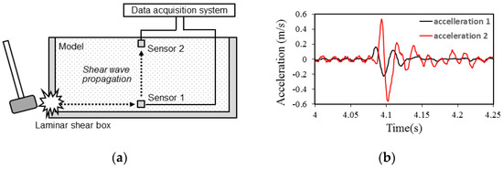
Figure 6.
The shear wave velocity measurement method used in this study: (a) shear wave generation by physical impact; (b) output signals of two accelerometers.
For a single-layer ground model, in order to measure the shear wave velocity, the hammer test should be carried out on the outer side of the soft soil bottom end to measure the average shear wave velocity of the ground. However, for the multilayered flat model ground, the thickness of each layer is less than 0.3 m. Since the impact of the hammer will pass through the ground at a faster rate than the data collection interval, the accuracy of the average breaking wave velocity calculated by the hammer test has decreased. In order to make up for this defect, each layer of the multilayered ground was formed into a single soil layer with a thickness of 0.6 m, and the hammer tests were carried out separately to obtain the average shear wave velocity. Kaklamanos and Bradley [15] proposed a shear wave velocity map, which represents the upper and lower layers of the surface in Equation (2).
where is the shear wave velocity at depth z, is the average shear wave velocity in the layer, is the effective normal stress at the depth z, is the effective normal stress calculated in the middle of the layer and n is the stress index. The n value of clay, silky, and sandy soils are 1/3, the n value of gravel and rock are 1/4. A total of three hammer tests were conducted, with ten hammer strikes per test. The values of obvious errors were excluded and the average value was taken.
Figure 7 shows the acceleration-time history of the multilayered upper ground (loose ground) as a single layer ground with a thickness of 0.6 m, and the hammer test was performed by embedding an accelerometer in the bottom and surface layers of the soil. The average shear wave velocity of the layer was determined using the time difference between the first peaks and the distance between the buried accelerometer, and the average shear wave velocity obtained by repeating the hammer test was 76.57 m/s, 70.75 m/s and 68.75 m/s, and their average value, 72.02 m/s, was determined as the average shear wave velocity of loose ground.
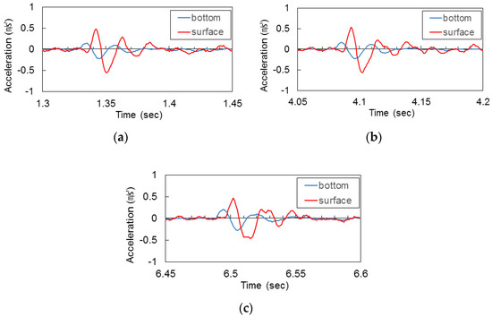
Figure 7.
Hammer test result: (a) Hammer test 1st; (b) Hammer test 2nd; (c) Hammer test 3rd.
Figure 8 shows the acceleration-time history of the multilayered lower ground (dense ground) as a single layer ground with a thickness of 0.6 m, and the hammer test was performed by embedding an accelerometer in the bottom and surface layers of the soil. The average shear wave velocity of the layer was determined using the time difference between the first peaks and the distance between the buried accelerometer; the average shear wave velocities obtained by repeating the hammer test were 139.80 m/s, 138.74 m/s and 133.96 m/s, and the average value of 137.5 m/s was determined as the average shear wave velocity of the dense ground.
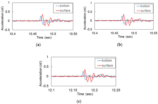
Figure 8.
Hammer test result: (a) hammer test 1st; (b) hammer test 2nd; (c) hammer test 3rd.
The shear wave velocity modulus of loose ground and dense ground formed by stratification was applied as shown in Figure 9.
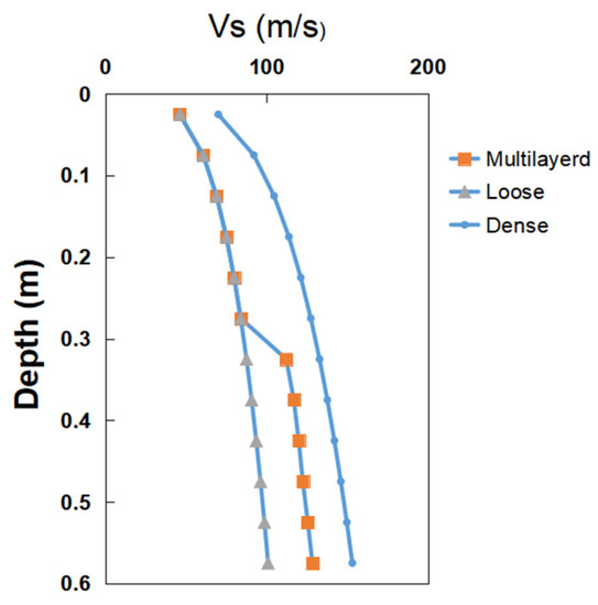
Figure 9.
The shear wave velocity modulus of loose ground and dense ground.
The shear wave velocity at the lower part of the single ground receives a higher vertical stress than the shear wave velocity at the lower part of the multilayered ground. Since the upper part of the multilayered ground is made of loose ground with low unit weight, and the vertical loading was applied to the lower part, so the shear wave velocity of the multilayered ground is lower than the shear wave velocity of the dense ground.
3.2. Peak Ground Acceleration
To evaluate the amplification characteristics of the multilayered flat model ground, the peak ground acceleration (PGA), spectral acceleration (SA), and amplification factor for the three input seismic waves were analyzed. Figure 10 shows the PGA by depth measured at the center of the flat, multilayered ground model. Under the three waveforms, the depth range of 0.3–0.6 m is dense ground, and the peak ground acceleration changes little with the decrease in depth. The depth range of 0–0.3 m is loose ground, and the peak ground acceleration increases obviously with the decrease in depth. Among them, the Sine 10 Hz wave does not show a steep shape even on the upper ground, because it is different from the natural period of the ground and cannot generate resonance. Artificial seismic waves and the sine wave resonate in the upper ground.
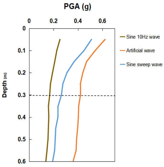
Figure 10.
Peak ground acceleration by depth of flat model under different seismic waves.
3.3. Response Spectral Acceleration
Figure 11 represents the depth-specific response spectral and response spectral amplification coefficients of the multilayered, flat ground model. The amplification factor showed the degree of amplification within 10 cm thickness by dividing the soil layer into 10 cm intervals for detailed identification. Figure 11a–l present the experimental results for the sine 10 Hz wave, the artificial seismic wave, and the sine sweep wave, respectively. Figure 11a,e,i show response spectral acceleration, and it can be seen that the acceleration is amplified according to the vertical height. Figure 11c,g,k are the response spectral amplification coefficients of the upper ground, and it was confirmed that in the loose ground, the amplification was about 1.5 times for each layer thickness. In contrast, as shown in Figure 11b,f,j it was confirmed that amplification hardly occurred in the dense ground. In Figure 11d,h,l the amplification of the inter-layer boundary of the multi-layered ground was compared with the amplification factor of the upper and lower ground. At the inter-layer boundary, it was amplified halfway between the bottom and the top.
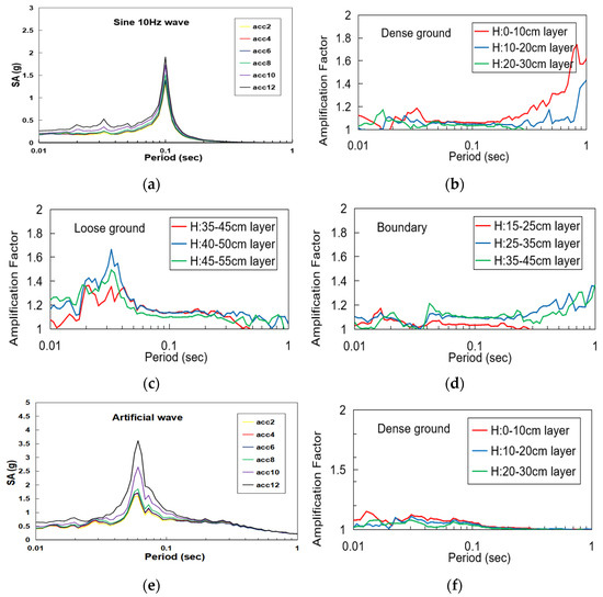
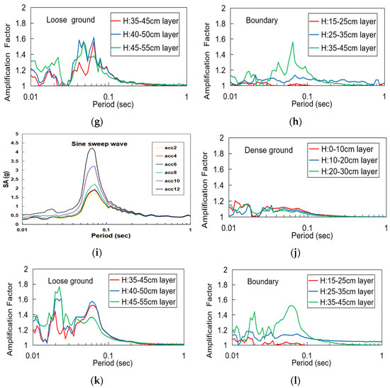
Figure 11.
Spectral response acceleration for measured ground motion at different depths: (a) SA by sine 10 Hz; (b) AF of dense ground by sine 10 Hz; (c) AF of loose ground by sine 10 Hz; (d) AF of boundary ground by sine 10 Hz; (e) SA by artificial wave; (f) AF of dense ground by artificial wave; (g) AF of loose ground by artificial wave; (h) AF of boundary ground by artificial wave; (i) SA by sine sweep; (j) AF of dense ground by sine sweep; (k) AF of loose ground by sine sweep; (l) AF of boundary ground by sine sweep.
4. Comparison and Analysis of Response Acceleration Results between the Experiment and Numerical Simulation Model
4.1. One-Dimensional Ground Response Numerical Simulation Model
In order to calibrate and validate the overall reliability of the shaking table test results utilized in this study, a one-dimensional ground response analysis was performed for the flat ground model created in the laminar shear box. The ground response analysis was performed using the open-source software DEEPSOIL, version 7 of the University of Illinois at Urbana-Champaign (UIUC) and analyzed in a nonlinear way [16]. The compositional models were the general quadratic/hyperbolic (GQ/H) ground model and the non-masing hysteresis model.
The parameters contained in the model by DEEPSOIL software are shown in Table 4 (because there are twelve layers in total, the first layer is the main display data and the input data of each layer are also displayed below). The Darendeli constitutive model is used for modeling and nonlinear analysis, and the acceleration-time history and 5% damped spectral acceleration according to ASCE standard were obtained [17], which can be used to explore the dynamic characteristics of soil.
Table 4.
Parameter of the DEEPSOIL used in this study.
The model was characterized by a total cross-sectional depth of 60 cm, according to the actual size of the experimental model, and 12 layers with a thickness of every 5 cm from the surface to the bottom were defined. Six layers from the surface to a depth of 30 cm were modeled with loose ground with a unit weight of 14.715 kN/m3, while six layers from 30 cm to 60 cm were modeled with dense ground with a unit weight of 19.62 kN/m3.
The shear strength was calculated by depth according to the Mohr-Coulomb failure line [18] according to Equation (3).
where, is the shear strength, is the cohesion, is the normal stress, and is the internal friction angle.
The specific modeling interface and parameters of each layer are shown in Figure 12.
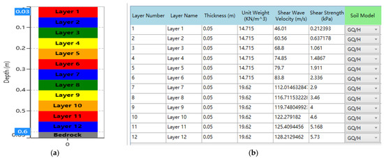
Figure 12.
DEEPSOIL software: (a) Modeling in DEEPSOIL; (b) parameters of each layer.
In 1972, Hardin and Drnevich [19] proposed a hyperbolic shear modulus reduction function and an approximate shape for the material damping curve for soil. Based on Hardin-Drnevich model, Darendeli [20] proposed a modified hyperbolic model as Equation (4). The curvature coefficient a is integrated into the normalized modulus reduction curve.
where, is the , is , is and α is the regression parameter.
Figure 13 shows normalized shear modulus reduction and material damping ratio curves of loose soil and dense soil by Darendeli constitutive model in DEEPSOIL.

Figure 13.
Normalized soil shear modulus and material damping ratio relationship.
4.2. Comparison of Numerical Analysis Results and Shaking Table Test Results
The response data of the accelerometer buried deep in the center of the multilayered, flat ground model and the one-dimensional ground response analysis results were compared through the peak ground acceleration and spectral acceleration curves.
Figure 14 compared the peak ground acceleration for each input wave. For the peak ground acceleration, it was confirmed that the experiment and numerical analysis results of each input seismic shaking were generally consistent, but acceleration obtained by numerical analysis was less than the experimental value at the top. This is considered to be because the acceleration at the top layer of the model increases due to resonance in the process of shear wave velocity measurement, which resulted in increase of shear wave velocity. During the hammer test, the soil layer in the soil box will settle to a certain extent due to gravity and shock, resulting in a decrease in height and an increase in frequency, which just produces an enhancement effect with part of the artificial seismic waves and sine sweep wave. The objective of this paper is to compare the variation and difference of acceleration amplification characteristics at different layer and inter-layer boundary. Therefore, the difference in PGA at the top layer does not greatly affect the comparison results and conclusions. Other than this, it seems that the PGA of the numerical analysis was predicted well.
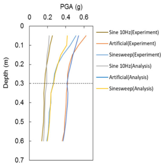
Figure 14.
Peak ground acceleration from the bottom to the surface under different input waves by experiment results and numerical analysis results.
Figure 15, Figure 16 and Figure 17 present the spectral acceleration amplification for the same input wave at different depths. Figure 15 exhibits the sine wave of each layer at 10 Hz between experiment and numerical analysis comparisons. As the depth is close to the surface, the value of spectral acceleration increases. Figure 15a–c shows that, from a depth of 0.2 m from the surface, as the height increases, the difference between the experimental results and the numerical analysis results keeps increasing and the SA of the experiment is always greater than that of the numerical analysis result. Figure 15d–f shows that the difference between the experiment results and the numerical analysis results is very close with a depth of 0.3 m.
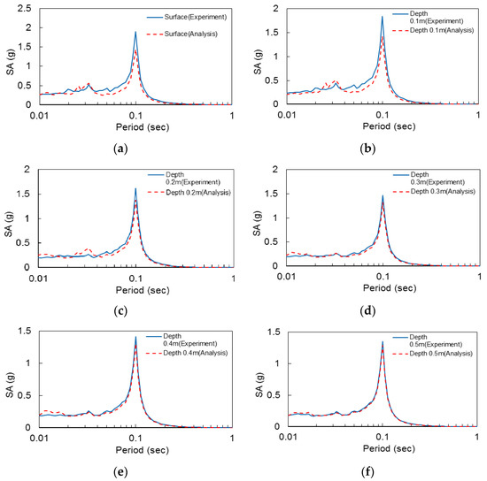
Figure 15.
(a) SA by sine 10 Hz wave at Surface; (b) SA by sine 10 Hz at 0.1 m depth; (c) SA by sine 10 Hz at 0.2 m depth; (d) SA by sine 10 Hz at 0.3 m depth; (e) SA by sine 10 Hz at 0.4 m depth; (f) SA by sine 10 Hz at 0.5 m depth.
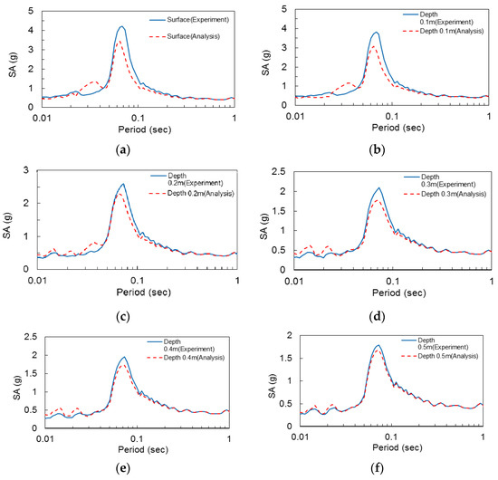
Figure 16.
(a) SA by sine sweep at surface; (b) SA by sine sweep at 0.1 m depth; (c) SA by sine sweep at 0.2 m depth; (d) SA by sines weep at 0.3 m depth; (e) SA by sine sweep at 0.4 m depth; (f) SA by sine sweep at 0.5 m depth.
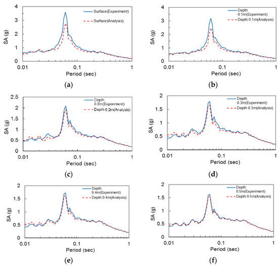
Figure 17.
(a) SA by artificial wave at surface; (b) SA by artificial wave at 0.1 m depth; (c) SA by artificial wave at 0.2 m depth; (d) SA by artificial wave at 0.3 m depth; (e) SA by artificial wave at 0.4 m depth; (f) SA by artificial wave at 0.5 m depth.
Figure 16 shows the sine sweep wave of each layer between experimental and numerical analysis comparisons. Figure 16a–f shows that, from bottom to the surface, as the height increases, the difference between the experiment results and the numerical analysis results keeps increasing and the SA of the experiment is always greater than that of the numerical analysis result. This trend is similar to what has been observed in the case of sine 10 Hz wave.
Figure 17 compares the experimental results and analytical values of the 1 g shaking table at different depths when the seismic wave is applied. The figure also shows that the 1D ground response analysis values of response spectral acceleration predict the experimental values well. The depth 0.3 to 0.5 m corresponding to dense ground has almost the same experimental value and analytical value. The response spectral acceleration of the depth surface to 0.3 m, which simulated the loose ground, was somewhat different from that of the dense ground, but overall it simulated the amplification well and predicted the main amplification cycle well. However, on the surface of the soft soil, the numerical analysis value is amplified less than the experimental value.
5. Summary and Conclusions
In order to experimentally confirm the acceleration amplification characteristics according to the difference in the physical properties of each layer in the multilayered ground and the amplification characteristics occurring at the inter-layer boundary, a scaled-down model experiment using the 1 g shaking table was performed to obtain the soil dynamic behavior. A dense lower ground was formed with a sample mixed with silica sand and sandy soil, and a loose upper ground was formed with sandy soil. Then, the acceleration was measured by applying a seismic loading through the 1 g shaking table test. The peak ground acceleration and spectral acceleration were shown with the measured response acceleration to illuminate the amplification change by depth of the scaled-down model and the amplification difference between each layer. In addition, calibrating and verifying the experimental results with DEEPSOIL results can make the experimental results more convincing and provide strong support for large-scale model analysis relying on the 1 g shaking table test by the law of similarity. In this study, the following conclusions were obtained:
- (1)
- In the absence of resonance, experimental results under a sine 10 Hz wave showed that the acceleration increase of loose ground is larger than that of dense ground on multilayered ground by PGA and SA. In the cases of artificial seismic waves and sine sweep waves, resonance appeared at the top of the experimental model, resulting in the increase of acceleration.
- (2)
- The response spectral acceleration confirmed that acceleration was amplified with depth decreases, that the upper ground amplification factor was more amplified on loose ground, and that the lower ground amplification factor was less amplified on dense ground. Compared to the amplification factor of the multilayered boundary, the inter-layer boundary was found to be amplified to the middle of the lower layers. Moreover, the spectral acceleration amplification factor of the inter-layer boundary is between that of the lower layer and the upper layer.
- (3)
- Comparing the experimental results and numerical analysis results of the 1 g shaking table at different depths, it could be seen that the dense ground with 0.3–0.5 m had almost the same experimental and numerical analysis results. In addition, the surface layer that simulates the loose ground layer from surface to 0.3 m has some differences compared to the dense ground, but it has been found to predict the main amplification cycle well.
- (4)
- As a result of mutual comparison with the one-dimensional ground response analysis using DEEPSOIL, it was confirmed that the peak ground acceleration was generally consistent with the experimental value of each input seismic shaking. In addition, the difference between the experimental results and the numerical analysis results increases with the increase in height. The accuracy of the data is guaranteed by using multiple waveforms to simulate the multilayered ground.
- (5)
- In this study, scaled-down model experiments were carried out based on a 1 g shaking table. Overall, the results obtained using the DEEPSOIL numerical analysis software compare well with the 1 g shaking table test results performed on multilayered ground. However, there are still some limitations in using DEEPSOIL. In the future, we will focus more on large-scale flat ground and slopes, use 2D/3D simulation software for numerical simulation analysis based on the 1 g shaking table test, and study actual cases to analyze the dynamic behavior of soil.
Author Contributions
Writing—original draft preparation, Y.J. and H.K.; Review and editing, D.K.; Date acquisition Y.J., S.J. and H.K. All authors have read and agreed to the published version of the manuscript.
Funding
This research was funded by Basic Science Research Program through the National Research Foundation of Korea (NRF) funded by the Ministry of Education (NRF-2021R1I1A3044804).
Institutional Review Board Statement
Not applicable.
Informed Consent Statement
Not applicable.
Data Availability Statement
Not applicable.
Conflicts of Interest
The authors declare no conflict of interest.
References
- Murao, H.; Nakai, K.; Noda, T.; Yoshikawa, T. Deformation–failure mechanism of saturated fill slopes due to resonance phenomena based on 1 g shaking-table tests. Can. Geotech. J. 2018, 55, 1668–1681. [Google Scholar] [CrossRef]
- Shinoda, M.; Watanabe, K.; Sanagawa, T.; Abe, K.; Nakamura, H.; Kawai, T.; Nakamura, S. Dynamic behavior of slope models with various slope inclinations. Soils Found. 2015, 55, 127–142. [Google Scholar] [CrossRef]
- Yang, J. Saturation effects on horizontal and vertical motions in a layered soil–bedrock system due to inclined SV waves. Soil Dyn. Earthq. Eng. 2001, 21, 527–536. [Google Scholar] [CrossRef]
- Wartman, J.; Seed, R.B.; Bray, J.D. Shaking table modeling of seismically induced deformations in slopes. J. Geotech. Geoenviron. Eng. 2005, 131, 610–622. [Google Scholar] [CrossRef]
- Brennan, A.J.; Madabhushi, S.P.G. Amplification of seismic accelerations at slope crests. Can. Geotech. J. 2009, 46, 585–594. [Google Scholar] [CrossRef]
- Abe, K.; Nakamura, S.; Nakamura, H.; Shiomi, K. Numerical study on dynamic behavior of slope models including weak layers from deformation to failure using material point method. Soils Found. 2017, 57, 155–175. [Google Scholar] [CrossRef]
- Hou, C.; Zhang, T.; Sun, Z.; Dias, D.; Shang, M. Seismic analysis of nonhomogeneous slopes with cracks using a discretization kinematic approach. Int. J. Geomech. 2019, 19, 04019104. [Google Scholar] [CrossRef]
- Goktepe, F.; Celebi, E.; Omid, A.J. Numerical and experimental study on scaled soil-structure model for small shaking table tests. Soil Dyn. Earthq. Eng. 2019, 119, 308–319. [Google Scholar] [CrossRef]
- Song, D.; Che, A.; Zhu, R.; Ge, X. Natural frequency characteristics of rock masses containing a complex geological structure and their effects on the dynamic stability of slopes. Rock Mech. Rock Eng. 2019, 52, 4457–4473. [Google Scholar] [CrossRef]
- Zhang, J.; Yuan, Y.; Yu, H. Shaking table tests on discrepant responses of shaft-tunnel junction in soft soil under transverse excitations. Soil Dyn. Earthq. Eng. 2019, 120, 345–359. [Google Scholar] [CrossRef]
- Nakamura, S. Analysis of behavior of slope models for collapsing from stability by shaking table tests under 1G field. In MATEC Web of Conferences; EDP Sciences: Les Ulis, France, 2019; Volume 258, p. 05004. [Google Scholar]
- Jin, Y.; Kim, H.; Kim, D.; Lee, Y.; Kim, H. Seismic Response of Flat Ground and Slope Models through 1 g Shaking Table Tests and Numerical Analysis. Appl. Sci. 2021, 11, 1875. [Google Scholar] [CrossRef]
- Kim, H.; Kim, D.; Lee, Y.; Kim, H. Effect of soil box boundary conditions on dynamic behavior of model soil in 1 g shaking table test. Appl. Sci. 2020, 10, 4642. [Google Scholar] [CrossRef]
- Sun, C.G.; Han, J.T.; Cho, W. Representative shear wave velocity of geotechnical layers by synthesizing in-situ seismic test data in Korea. J. Eng. Geol. 2012, 22, 293–307. [Google Scholar] [CrossRef][Green Version]
- Kaklamanos, J.; Bradley, B.A. Challenges in predicting seismic site response with 1D analyses: Conclusions from 114 KiK-net vertical seismometer arrays. Bull. Seismol. Soc. Am. 2018, 108, 2816–2838. [Google Scholar] [CrossRef]
- Hashash, Y.M.A.; Musgrove, M.I.; Harmon, J.A.; Ilhan, O.; Xing, G.; Numanoglu, O.; Groholski, D.R.; Phillips, C.A.; Park, D. DEEPSOIL 7.0, User Manual; Board of Trustees of University of Illinois at Urbana-Champaign: Urbana, IL, USA, 2020. [Google Scholar]
- American Society of Civil Engineers. Minimum Design Loads and Associated Criteria for Buildings and Other Structures; American Society of Civil Engineers: Reston, VA, USA, 2022. [Google Scholar]
- Labuz, J.F.; Zang, A. Mohr–coulomb failure criterion. In The ISRM Suggested Methods for Rock Characterization, Testing and Monitoring: 2007–2014; Springer: Cham, Switzerland, 2012; pp. 227–231. [Google Scholar]
- Hardin, B.O.; Drnevich, V.P. Shear modulus and damping in soils: Design equations and curves. J. Soil Mech. Found. Div. 1972, 98, 667–692. [Google Scholar] [CrossRef]
- Darendeli, M.B. Development of a New Family of Normalized Modulus Reduction and Material Damping Curves; The university of Texas at Austin: Austin, TX, USA, 2001. [Google Scholar]


Publisher’s Note: MDPI stays neutral with regard to jurisdictional claims in published maps and institutional affiliations. |
© 2022 by the authors. Licensee MDPI, Basel, Switzerland. This article is an open access article distributed under the terms and conditions of the Creative Commons Attribution (CC BY) license (https://creativecommons.org/licenses/by/4.0/).