A Lyapunov Stability Analysis of Modified HOSM Controllers Using a PID-Sliding Surface Applied to an ABS Laboratory Setup

Abstract

The antilock braking system (ABS) is a mechatronic system that helps a driver maintain the maneuverability of a vehicle while braking by preventing wheel lock-ups. However, the design of high-performance controllers for this type of system is complicated because of its highly nonlinear dynamics. The problem becomes even more difficult to resolve when uncertainties in the parameters appear in its dynamics. In this paper, an ABS laboratory setup mimicking a quarter car model is considered. A modified high-order sliding mode (HOSM) controller using a proportional-integral-differential (PID) control as a sliding surface was designed. This controller provides a reference value of a tire slip. The proposed controller uses a tracking error to define the slip surface through the PID controller structure, and the modified HOSM controller holds the system on the previously designed slip surface. The closed-loop system stability has been proven in the sense of Lyapunov. Finally, the ABS laboratory setup allows for experimentally checking the performance of the modified HOSM controller using a PID-sliding surface, showing a considerable increase in the efficiency of the control system compared with a PID-like controller.

1. Introduction

The antilock braking system (ABS) is an electronically controlled system that helps a driver maintain control of a vehicle during emergency braking by preventing the wheels from locking up. This prevents the slippage of the wheels on a surface by regulating the brake-fluid pressure of each wheel. Acting on the brake pressure, ABS control algorithms usually impose an appropriate wheel acceleration or a desired tire slip, i.e., a certain relative difference in the wheel with respect to the vehicle velocity.

In any case, the ABS control design is challenged by the fact that the ABS’s performance can be drastically affected by disturbances in the dynamics of the ABS. For this reason, sliding-mode control (SMC) is considered an ideal solution for the ABS due to its robustness to disturbances and parameter uncertainties. In addition, the fast, dynamic response of SMC fulfills the real-time requirements of the ABS, but the main problem with the application of SMC is a chattering phenomenon. However, the HOSM technique [1] avoids some of the typical problems of the classic SMC technique [2], such as the chattering phenomenon noted above.

One remarkable feature of the HOSM is that sliding-mode surfaces with relative degrees greater than one can be considered [3]. Since the creation of this technique, a number of articles have been published about the HOSM [4,5,6,7]. Initially, HOSM techniques were used for smooth control systems, but recently, they have been applied to finite-time differentiators. In [8], an interesting comparison of HOSM differentiators and high-gain observers concerning measurement noise was made. Some HOSM application techniques for solving vehicle-control problems can be found in [9,10,11], and references [12,13,14,15] presented several fields and practical cases for which these techniques were applied successfully.

However, despite the current knowledge about HOSM controllers, in recent years, scientists have proposed a combination of the HOSM controller and PI/PID-sliding surfaces. Some examples can be found in the literature; reference [16] investigated an adaptive fault-tolerant pseudo-PID–SMC scheme for a high-speed train subjected to actuator-fault asymmetric nonlinear actuator saturation. In [17], a combination of SMC with a traditional PID control scheme for a two-degrees-of-freedom planar manipulator was considered. In [18], an SMC scheme for the robust tracking control of the nanopositioning stage composed of piezoceramic stack-actuator-compliant flexure mechanisms using a PID-type sliding surface was presented. In [19], a second-order SMC with a PI-sliding surface for a DC motor-driven control was designed. Reference [20] applied an SMC with a PID-sliding surface to the active vibration damping of pneumatically actuated soft robots. Reference [21] considered the design of a modified HOSM controller using a PI-sliding surface for the attitude control of a ground vehicle. Reference [22] developed an adaptive dynamic PID-sliding surface-based second-order fault-tolerant SMC for the speed control of an electromechanical system. Reference [23] considered a second-order SMC with a PID-sliding surface applied to a modified dynamic model of a quad-rotor UAV with the disturbance of an unbalanced load.

In the present work, a modified HOSM using a PID control as a sliding surface is designed to impose a reference value of a tire slip. An ABS setup is used to experimentally test new control laws [24]. It consists of a lower aluminum wheel, simulating a vehicle’s longitudinal motion, and an upper plastic wheel, simulating the vehicle’s wheel. The velocity of the lower wheel, i.e., the vehicle’s longitudinal velocity, is changed using a large DC motor coupled with the wheel. The velocity of the upper wheel, i.e., the wheel’s angular velocity, is diminished by using a disk-brake system, which is operated by using a small DC motor for which the control input is applied. In the case of the incipient lock-up of the upper wheel, an electronic control unit reduces the pressure in the disk-brake system via an electronic modulator.

Recently, various studies used this ABS setup. For example, References [25,26] compared linear and nonlinear controllers. In [27,28], an adaptive controller that estimates the tire–road adhesion coefficient was developed. References [29,30,31] presented some fuzzy controllers, and reference [32] proposed intelligent control techniques applied to an adaptive neuro-fuzzy controller. Reference [33] provided a nonlinear observer to recreate a vehicle’s longitudinal velocity, as was shown in [34], to develop a dynamic controller that imposes a specific wheel-slip ratio. A plain variant of this control was carried out through a linearized event-triggered strategy in [35]. Reference [36] presented their design and application to the ABS laboratory of the Lyapunov-based SMC and reaching-law-based SMC. In [37], the real-time implementation of the super-twisting controller for the ABS laboratory setup was developed using a super-twisting estimation to provide a finite-time estimation of the tire–road friction coefficient.

In this article, a modified HOSM controller using a PID-sliding surface is designed and applied to the ABS laboratory setup to track a suitable value of the wheel-slip ratio. Hence, the original contributions of the present paper are as follows:

• A modified HOSM controller using a PID-sliding surface was designed.
• The convergence and stability of the controller were proven rigorously using a theoretical analysis based on the Lyapunov function.
• The proposed controller was implemented in an ABS laboratory setup, and the results were compared with a PID-like controller.

The rest of this paper is organized as follows. Section 2 describes the mathematical modeling of the ABS laboratory setup. Section 3 discusses the control problem and the proposed modified HOSM using a PID-sliding surface. The numerical and real-time simulations are presented in Section 4. Finally, the conclusion summarizes this paper.

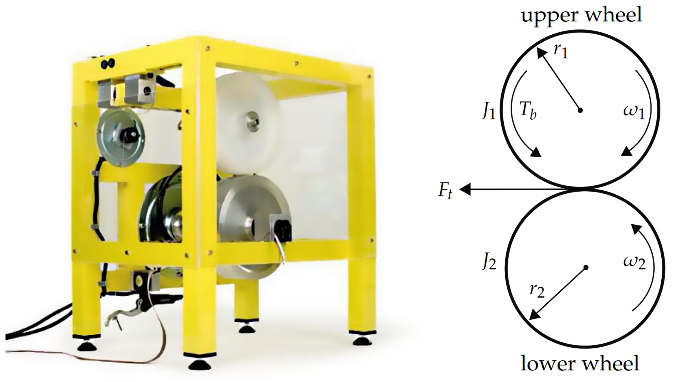
2. Mathematical Model of the Experimental ABS Laboratory Setup

The Inteco experimental setup is the mechatronic system studied in this article (see Figure 1) that simulates the mechanics of a quarter of an actual vehicle. As already commented upon, the setup comprises a lower aluminum wheel representing road motion and an upper plastic wheel that emulates a vehicle wheel. A DC motor is coupled to accelerate the lower wheel, whereas the upper wheel is equipped with a disk-brake system. The positions of the two wheels are obtained through encoders, and the wheels’ velocities are obtained through numerical differentiation. Despite its simplicity, this setup keeps the essential features of a functional ABS in the range of 0–70 km/h [24].

Mathematical Model of the Experimental ABS Laboratory Setup

The mathematical model of the ABS experimental setup was developed under the assumptions of imperceptible lateral and vertical dynamics and negligible rolling resistance force with respect to braking. The dynamic equations of the experimental setup were as follows [24,27,28]:

$$\begin{array}{cc}\hfill {\dot{\omega }}_1& =\frac{r_1}{J_1}{F}_t-\frac{1}{J_1}\left(d_1{\omega }_1+T_b\right)\hfill \\ \hfill {\dot{\omega }}_2& =-\frac{r_2}{J_2}{F}_t-\frac{1}{J_2}{d}_2{\omega }_2\hfill \end{array}$$

(1)

where ${\omega }_1$ and ${\omega }_2$ represented the angular velocities of the upper and lower wheels, respectively; $J_1$ and $J_2$ were inertia moments; and $r_1$ and $r_2$ were the radii. Moreover, $d_1$ and $d_2$ were the coefficients of the viscous friction of the upper and lower wheel, respectively (the nominal parameters are given in

Table 1. Parameters of the experimental setup.

Symbol	Value	Unit
$r_1$	0.0995	m
$r_2$	0.0990	m
$J_1$	$7.54\times {10}^{-3}$	kg m${}^2$
$J_2$	$25.6\times {10}^{-3}$	kg m${}^2$
$d_1$	$118.74\times {10}^{-6}$	kg m${}^2$/s
$d_2$	$214.68\times {10}^{-6}$	kg m${}^2$/s
$\mu$	1
$b_1$	15.24
$b_0$	6.21
c	20.37	s${}^{-1}$
$u_0$	0.415
D	23
C	1.68
B	28

).

During the acceleration and braking processes, a longitudinal tire force $F_t$ is achieved during contact between the upper and lower wheels (see Figure 1). This traction force is proportional to the usual load of the vehicle via the tire–road friction coefficient $\mu \in [0,1]$ and is a nonlinear function of the longitudinal wheel-slip ratio, i.e., the relative velocity difference:

$$\lambda =\frac{v_x-v_w}{v_x}=\frac{r_2{\omega }_2-r_1{\omega }_1}{r_2{\omega }_2}=1-\frac{r_1}{r_2}\frac{{\omega }_1}{{\omega }_2}$$

(2)

where the quantities $v_x=r_2{\omega }_2$ and $v_w=r_1{\omega }_1$ represent the vehicle longitudinal velocity and the vehicle wheel velocity, respectively. According to [24], $T_b$ is the braking torque and is designed by using a first-order equation:

$${\dot{T}}_b=c\left(-T_b+b\left(u\right)\right)$$

(3)

where $c>0$ is a constant and $b\left(u\right)$ is the control input that expresses the relationship between u and the voltage applied to the coupled DC motor (which drives the action of the brake pads). This relation can be calculated using an equation comparable with the brake-pedal model in a vehicle [25,34,38]:

$$b\left(u\right)=\left\{\begin{array}{cc}{b}_{1}u-b_0& \mathrm{if} u\ge u_0\\ 0\hfill & \mathrm{if} u<u_0\end{array}\right.$$

where $u_0$ is the operating threshold of the brake-driving system and $b_1$ and $b_0$ are constants. In this case, the control signal u is the voltage applied to the small DC motor. This motor commands brake pads located in the upper wheel. Considering the constant steady-state value $T_b$ in (3), the control signal u can be obtained by solving for $u=(T_b+b_0)/b_1$.

Additionally, to design the traction force $F_t$ in the linear and nonlinear region, in this paper, the widely used Pacejka’s magic formula [39] model was selected. This method approaches the response curve of the braking process based on experimental data.

Then, the traction force is defined as follows:

$$F_t=\mu D\sin \left(C\arctan \left(B\lambda \right)\right)$$

(4)

where $\mu$ is the friction coefficient between the two wheels and simulates road conditions and the coefficients B, C, and D are determined experimentally.

Hence, considering (3) and the definition (4), the dynamic equations of the ABS laboratory setup (1) can be rewritten in the following form:

$$\begin{array}{cc}\hfill {\dot{\omega }}_1& =\frac{r_1}{J_1}{F}_t-\frac{1}{J_1}\left(d_1{\omega }_1+T_b\right)\hfill \\ \hfill {\dot{\omega }}_2& =-\frac{r_2}{J_2}{F}_t-\frac{1}{J_2}{d}_2{\omega }_2\hfill \\ \hfill {\dot{T}}_b& =c(-T_b+b\left(u\right)).\hfill \end{array}$$

(5)

3. A Modified HOSM Controller Using a PID-Sliding Surface for an ABS Laboratory Setup

The primary function of a controller is to prevent the vehicle wheel from being locked during emergency braking and to maintain the slip ratio at a value of ${\lambda }_{\mathrm{ref}}$ corresponding to the maximum $F_{t,\max }=F_t$ of the force $F_t$ (4). Consequently, the slip reference remains fixed to ${\lambda }_{\mathrm{ref}}=F_t^{-1}\left(F_{t,\max }\right)$. Hence, considering this reference value, the output signal to be controlled is the wheel slip $\lambda$, and the control problem is designing a controller such that $\lambda$ (2) can track the desired reference ${\lambda }_{\mathrm{ref}}$ in the presence of uncertainties in the parameters. Thus, the control problem can be solved under the following assumption:

Assumption 1.

The angular velocities ${\omega }_1$ and ${\omega }_2$ are considered measurable.

In the following section, the modified HOSM control using a PID-sliding surface is designed to solve the control problem in such a way that the slip-error converges $e_{\lambda }=\lambda -{\lambda }_{\mathrm{ref}}$ to zero. Let us propose the slip velocity $v_s=v_x-v_w=\lambda v_x$, the slip-velocity reference $v_{s,\mathrm{ref}}={\lambda }_{\mathrm{ref}}{v}_x$, and the slip-velocity error:

$$e_v=v_s-v_{s,\mathrm{ref}}=e_{\lambda }{v}_x=(1-{\lambda }_{\mathrm{ref}})v_x-v_w.$$

(6)

Since $v_x\ne 0$, the control problem is comparable with drive $e_v$ to zero, where the dynamics of the slip velocity error are as follows:

$$\begin{array}{c}{\dot{e}}_v=(1-{\lambda }_{\mathrm{ref}}){\dot{v}}_x-{\dot{v}}_w=(1-{\lambda }_{\mathrm{ref}})r_2{\dot{\omega }}_2-r_1{\dot{\omega }}_1\hfill \\ =-k\left({\lambda }_{\mathrm{ref}}\right)F_t+\frac{r_1}{J_1}{d}_1{\omega }_1-(1-{\lambda }_{\mathrm{ref}})\frac{r_2}{J_2}{d}_2{\omega }_2+\frac{r_1}{J_1}{T}_b\hfill \end{array}$$

(7)

with $k\left({\lambda }_{\mathrm{ref}}\right)=\frac{r_1^2}{J_1}+(1-{\lambda }_{\mathrm{ref}})\frac{r_2^2}{J_2}$.

Then, the second derivative of the slip-velocity error (6) is as follows:

$$\begin{array}{cc}\hfill {\ddot{e}}_v& =-k\left({\lambda }_{\mathrm{ref}}\right){\dot{F}}_t+\frac{r_1}{J_1}{d}_1{\dot{\omega }}_1-(1-{\lambda }_{\mathrm{ref}})\frac{r_2}{J_2}{d}_2{\dot{\omega }}_2+\frac{r_1}{J_1}{\dot{T}}_b\hfill \\ \hfill =& -k\left({\lambda }_{\mathrm{ref}}\right){\dot{F}}_t+k_F{F}_t-k_{\omega ,1}{\omega }_1+k_{\omega ,2}{\omega }_2-k_T{T}_b+k_{u}b\left(u\right)\hfill \\ \hfill {\ddot{e}}_v& =f_v+k_{u}b\left(u\right)\hfill \end{array}$$

(8)

where

$$\begin{array}{cc}\hfill f_v& =-k\left({\lambda }_{\mathrm{ref}}\right){\dot{F}}_t+k_F{F}_t-k_{\omega ,1}{\omega }_1+k_{\omega ,2}{\omega }_2-k_T{T}_b\hfill \\ \hfill k_F& =\frac{r_1^2}{J_1^2}{d}_1+(1-{\lambda }_{\mathrm{ref}})\frac{r_2^2}{J_2^2}{d}_2;\hfill \\ \hfill k_{\omega ,1}& =\frac{r_1}{J_1^2}{d}_1^2;k_{\omega ,2}=(1-{\lambda }_{\mathrm{ref}})\frac{r_2}{J_2^2}{d}_2^2;\hfill \\ \hfill k_T& =\frac{r_1}{J_1^2}{d}_1+\frac{r_1}{J_1}c;k_u=\frac{r_1}{J_1}c.\hfill \end{array}$$

(9)

3.1. Design of the PID-Sliding Surface

The classic PID controller is defined as [40]

$$U_{PID}=k_{p}e\left(t\right)+k_i{\int }_0^{t}e\left(\tau \right)\mathrm{d}\tau +k_d\dot{e}\left(t\right)$$

(10)

where the controller parameters $k_p$, $k_i$, and $k_d$ are the proportional, integral, and derivative gains.

Using the classic PID controller (10) as the sliding surface and based on the slip-velocity error (6), the PID-sliding surface is defined as follows:

$$s_v=k_p{e}_v\left(t\right)+k_i{\int }_0^t{e}_v\left(\tau \right)\mathrm{d}\tau +k_d{\dot{e}}_v\left(t\right)$$

(11)

where $k_p$, $k_i$, and $k_d$ are the design parameters for tuning the dynamic response of the system on the sliding surface. The first derivative, with respect to the time of the sliding surface (11), is thus as follows:

$${\dot{s}}_v=k_p{\dot{e}}_v+k_i{e}_v+k_d{\ddot{e}}_v.$$

(12)

Considering the slip-velocity error (6) and its derivatives (7) and (8) within (12), one obtains the following:

$${\dot{s}}_v=k_p{\dot{e}}_v+k_i{e}_v+k_d\left(f_v+k_{u}b\left(u\right)\right).$$

(13)

3.2. Design of the Modified HOSM Control Using a PID-Sliding Surface

In this subsection, the design of the modified HOSM control using a PID-sliding surface applied to the ABS laboratory configuration—and the proof of stability of the proposed controller based on a theoretical analysis of the Lyapunov function—are presented.

Theorem 1.

For the system (5) and under Assumption 1, based on the sliding surface defined in (11), the following controller provides the solution that the slip-velocity error $e_v$ (6) will asymptotically converge to zero.

$$\begin{array}{cc}\hfill b\left(u\right)& =-\frac{1}{k_d{k}_u}\left(k_p{\dot{e}}_v+k_i{e}_v+k_d{f}_v+{\gamma }_1{\lfloor s_v\rceil }^{1/2}+{\gamma }_2{s}_v-{\xi }_v\right)\hfill \\ \hfill {\dot{\xi }}_v& =-{\gamma }_3{\lfloor s_v\rceil }^0-{\gamma }_4{s}_v.\hfill \end{array}$$

(14)

This controller will force the system toward the slip surface even in the presence of parametric uncertainty if the gains ${\gamma }_1,{\gamma }_2,{\gamma }_3$, and ${\gamma }_4$ are selected, such that

$$\begin{array}{cc}\hfill {\gamma }_1,{\gamma }_2,{\gamma }_3,{\gamma }_4& >0\hfill \\ \hfill 4{\gamma }_3{\gamma }_4& >{\gamma }_2^2\left(8{\gamma }_3+9{\gamma }_1^2\right)\hfill \end{array}$$

(15)

and $k_p,k_i,k_d>0$, $f_v$ as in (9).

Proof. 

To obtain the differential inclusion that represents the derivative of a sliding surface, the control input (14) needs to be used in (13), such that

$$\begin{array}{cc}\hfill {\dot{s}}_v& =-{\gamma }_1{\lfloor s_v\rceil }^{1/2}-{\gamma }_2{s}_v+{\xi }_v\hfill \\ \hfill {\dot{\xi }}_v& =-{\gamma }_3{\lfloor s_v\rceil }^0-{\gamma }_4{s}_v\hfill \end{array}$$

(16)

with ${\gamma }_1,{\gamma }_2,{\gamma }_3$, and ${\gamma }_4>0$, ${\lfloor s_v\rceil }^{1/2}={\left|s_v\right|}^{1/2}\mathrm{sign}\left(s_v\right)$, and ${\lfloor s_v\rceil }^0=\mathrm{sign}\left(s_v\right)$.

From [41], the following Lyapunov function is considered:

$$\mathcal{V}=2{\gamma }_3\left(\right|s_v\left|\right)+{\gamma }_4{s}_v^2+\frac{1}{2}{\xi }_v+\frac{1}{2}{\left({\gamma }_1{\lfloor s_v\rceil }^{1/2}+{\gamma }_2{s}_v-{\xi }_v\right)}^2$$

in which $\mathcal{V}$ is a continuous and differentiable Lyapunov function when $s_v\ne 0$.

The Lyapunov function can be written as a quadratic form:

$$\mathcal{V}=\frac{1}{2}{\chi }^{T}P\chi ;$$

(17)

where

$$\chi =\left(\begin{array}{c}\hfill {\lfloor s_v\rceil }^{1/2}\\ s_v\\ {\xi }_v\end{array}\right);P=\left(\begin{array}{ccc}{\gamma }_1^2+4{\gamma }_3& {\gamma }_1{\gamma }_2& -{\gamma }_1\\ {\gamma }_1{\gamma }_2& 2{\gamma }_4+{\gamma }_2^2& -{\gamma }_2\\ -{\gamma }_1& -{\gamma }_2& 2\end{array}\right)>0$$

since ${\gamma }_1,{\gamma }_2,{\gamma }_3$, and ${\gamma }_4>0$.

Following [41], note that

$${\lambda }_{min}^P{\left|\right|\chi \left|\right|}_2^2\le \mathcal{V}\le {\lambda }_{max}^P{\left|\right|\chi \left|\right|}_2^2$$

(18)

where ${\lambda }_{min}^P,{\lambda }_{max}^P$ are the minimum and maximum eigenvalues of P, respectively.

Let $\dot{\chi }$ be the derivative with respect to the time of $\chi$ as follows:

$$\dot{\chi }=\left(\begin{array}{c}\frac{\mathrm{d}}{\mathrm{dt}}{\lfloor s_v\rceil }^{1/2}\\ \dot{s_v}\\ {\dot{\xi }}_v\end{array}\right)=-\frac{1}{2|s_v{|}^{1/2}}{\Lambda }_1\chi +\frac{1}{2}{\Lambda }_2\chi$$

(19)

Then, the derivative of the Lyapunov function (17) using (19) is as follows:

$$\begin{array}{cc}\hfill \dot{\mathcal{V}}& =-\frac{1}{2|s_v{|}^{1/2}}{\chi }^{T}P{\Lambda }_1\chi +\frac{1}{2}{\chi }^{T}P{\Lambda }_2\chi \hfill \\ \hfill P{\Lambda }_1& =\left(\begin{array}{ccc}{\gamma }_1({\gamma }_1^2+2{\gamma }_3)& 0& -{\gamma }_1^2\\ {\gamma }_2({\gamma }_1^2-2{\gamma }_3)& 0& -{\gamma }_1{\gamma }_2\\ -{\gamma }_1^2& 0& {\gamma }_1\end{array}\right);\hfill & \hfill P{\Lambda }_2& =\left(\begin{array}{ccc}-{\gamma }_2(3{\gamma }_1^2+4{\gamma }_3)& -2{\gamma }_1({\gamma }_2^2-{\gamma }_4)& 2{\gamma }_1{\gamma }_2\\ -{\gamma }_1(3{\gamma }_2^2+4{\gamma }_4)& -2{\gamma }_2({\gamma }_2^2+{\gamma }_4)& (2{\gamma }_2^2+4{\gamma }_4)\\ 3{\gamma }_1{\gamma }_2& 2{\gamma }_2^2-4{\gamma }_4& -2{\gamma }_2\end{array}\right).\end{array}$$

(20)

Solving the first term of (20), i.e., $-\frac{1}{2|s_v{|}^{1/2}}{\chi }^{T}P{\Lambda }_1\chi$, we can rewrite it as follows:

$$\begin{array}{cc}\hfill -\frac{1}{2|s_v{|}^{1/2}}{\chi }^{T}P{\Lambda }_1\chi & =-\frac{1}{2|s_v{|}^{1/2}}({\gamma }_1(2{\gamma }_3+{\gamma }_1^2){\left({\lfloor s_v\rceil }^{1/2}\right)}^2-2{\gamma }_1^2{\lfloor s_v\rceil }^{1/2}{\xi }_v\hfill \\ \hfill & +{\gamma }_2({\gamma }_1^2-2{\gamma }_3){\lfloor s_v\rceil }^{1/2}{s}_v-{\gamma }_1{\gamma }_2{s}_v{\xi }_v+{\gamma }_1{\xi }_v^2)\hfill \end{array}$$

(21)

Since $-\frac{1}{2|s_v{|}^{1/2}}{\gamma }_2({\gamma }_1^2-2{\gamma }_3){\lfloor s_v\rceil }^{1/2}{s}_v=-\frac{1}{2}{\gamma }_2({\gamma }_1^2-2{\gamma }_3){\left({\lfloor s_v\rceil }^{1/2}\right)}^2$, the first term (21) is as follows:

$$\begin{array}{cc}\hfill -\frac{1}{2|s_v{|}^{1/2}}{\chi }^{T}P{\Lambda }_1\chi & \hfill =-\frac{1}{2|s_v{|}^{1/2}}{\chi }^T\left(\begin{array}{ccc}{\gamma }_1({\gamma }_1^2+2{\gamma }_3)& 0& -{\gamma }_1^2\\ 0& 0& -\frac{1}{2}{\gamma }_1{\gamma }_2\\ -{\gamma }_1^2& -\frac{1}{2}{\gamma }_1{\gamma }_2& {\gamma }_1\end{array}\right)\chi \\ & -\frac{1}{2}{\chi }^T\left(\begin{array}{ccc}{\gamma }_2({\gamma }_1^2-2{\gamma }_3)& 0& 0\\ 0& 0& 0\\ 0& 0& 0\end{array}\right)\chi .\hfill \end{array}$$

(22)

Similarly, the second term $\frac{1}{2}{\chi }^{T}P{\Lambda }_2\chi$ of (20) is as follows:

$$\begin{array}{cc}\hfill \frac{1}{2}{\chi }^{T}P{\Lambda }_2\chi & =\frac{1}{2}(-{\gamma }_2(3{\gamma }_1+4{\gamma }_3){\left({\lfloor s_v\rceil }^{1/2}\right)}^2-2{\gamma }_2({\gamma }_2^2+{\gamma }_4)s_v^2-2{\gamma }_2{\xi }_v^2\hfill \\ & -{\gamma }_1(5{\gamma }_2^2+2{\gamma }_4){\lfloor s_v\rceil }^{1/2}{s}_v+5{\gamma }_1{\gamma }_2{\lfloor s_v\rceil }^{1/2}{\xi }_v+4{\gamma }_2^2{s}_v{\xi }_v)\hfill \end{array}$$

If ${\lfloor s_v\rceil }^{1/2}{s}_v=\frac{1}{|s_v{|}^{1/2}}{s}_v^2$ and ${\lfloor s_v\rceil }^{1/2}{\xi }_v=\frac{1}{|s_v{|}^{1/2}}{s}_v{\xi }_v$, then the second term is rewritten in the matrix form:

$$\frac{1}{2}{\chi }^{T}P{\Lambda }_2\chi =-\frac{1}{2}{\gamma }_2{\chi }^T\left(\begin{array}{ccc}3{\gamma }_1^2+4{\gamma }_3& 0& 0\\ 0& 2({\gamma }_2^2+{\gamma }_4)& -2{\gamma }_2\\ 0& -2{\gamma }_2& 2\end{array}\right)\chi -\frac{1}{2|s_v{|}^{1/2}}{\gamma }_1{\chi }^T\left(\begin{array}{ccc}0& 0& 0\\ 0& 5{\gamma }_2^2+2{\gamma }_4& -\frac{5}{2}{\gamma }_2\\ 0& -\frac{5}{2}{\gamma }_2& 0\end{array}\right)\chi .$$

(23)

Finally, using (22) and (23), one rewrites (20) as the following:

$$\dot{\mathcal{V}}=-\frac{1}{2|s_v{|}^{1/2}}{\chi }^T{Q}_1\chi -{\chi }^T{Q}_2\chi$$

(24)

with

$$Q_1=\frac{{\gamma }_1}{2}\left(\begin{array}{ccc}({\gamma }_1^2+2{\gamma }_3)& 0& -{\gamma }_1\\ 0& 2{\gamma }_4+5{\gamma }_2^2& -3{\gamma }_2\\ -{\gamma }_1& -3{\gamma }_2& 1\end{array}\right);Q_2={\gamma }_2\left(\begin{array}{ccc}2{\gamma }_1^2+{\gamma }_3& 0& 0\\ 0& {\gamma }_2^2+{\gamma }_4& -{\gamma }_2\\ 0& -{\gamma }_2& 1\end{array}\right).$$

The derivative of the Lyapunov function (24) is negative definite if $Q_1,Q_2>0$. This condition is fulfilled if the gains are determined as in (15).

Now, in order to determine the convergence of the sliding surface to zero in finite time, it is necessary to denote ${\lambda }_{min}^{Q_1},{\lambda }_{min}^{Q_2}$ as the minimum eigenvalues of $Q_1,Q_2$, and one finally works out the following from (18) [42]:

$$\dot{\mathcal{V}}\le -\frac{1}{|s_v{|}^{1/2}}{\lambda }_{min}^{Q_1}{\left|\right|\chi \left|\right|}_2^2-{\lambda }_{min}^{Q_2}{\left|\right|\chi \left|\right|}_2^2$$

(25)

and

$$|s_v{|}^{1/2}\le {\left|\right|\chi \left|\right|}_2\le \sqrt{\frac{2\mathcal{V}}{{\lambda }_{min}^P}}$$

so that

$$-\frac{1}{|s_v{|}^{1/2}}\le -\frac{\sqrt{{\lambda }_{min}^P}}{\sqrt{2}}\frac{1}{{\mathcal{V}}^{1/2}}$$

Then,

$$\dot{\mathcal{V}}\le -\left({\kappa }_1{\mathcal{V}}^{1/2}+{\kappa }_2\mathcal{V}\right)$$

where

$${\kappa }_1=\sqrt{2{\lambda }_{min}^P}\frac{{\lambda }_{min}^{Q_1}}{{\lambda }_{max}^P};{\kappa }_2=2\frac{{\lambda }_{min}^{Q_2}}{{\lambda }_{max}^P}.$$

Using the comparison lemma [42], the Lyapunov function $\mathcal{V}$, and therefore $\left|\right|\chi \left|\right|$, converge to zero in a finite-time less or equal to $T_f=t_0+\ln {\left({\displaystyle \frac{{\kappa }_1+{\kappa }_2{\mathcal{V}}^{1/2}\left(0\right)}{{\kappa }_1}}\right)}^{2/{\kappa }_2}$ units of time. □

Remark 1.

PID controllers are usually preferred in industrial applications due to their good performances in terms of asymptotic stability and precision in steady state. For this reason, it is acceptable to compare the performance of the modified HOSM control using PID-sliding surface (14) with that of the following PID-like controller [11,26,37]. The aim of this PID-like controller is to cancel the nonlinear dynamics of the system and to incorporate a desired dynamic.

For this purpose, one uses the Equations (6), (7) and (9), and the PID-like controller [43] is as follows:

$$\begin{array}{cc}\hfill {\dot{I}}_v& =e_v\hfill \\ \hfill b\left(u\right)& =\frac{1}{k_u}\left(-k_{p,c}{e}_v-k_{i,c}{I}_v-k_{d,c}{\dot{e}}_v-f_v\right)\hfill \end{array}$$

(26)

so that from (8) and (26), one obtains the closed-loop dynamics

$$\begin{array}{c}\hfill {\ddot{e}}_v=-k_{p,c}{e}_v-k_{i,c}{I}_v-k_{d,c}{\dot{e}}_v\end{array}$$

(27)

where the gains $k_{p,c}$, $k_{d,c}$, and $k_{i,c}$ are $>0$ ensure the global exponential closed-loop stability of the error dynamics ${\ddot{e}}_v+k_{p,c}{e}_v+k_{i,c}{I}_v+k_{d,c}{\dot{e}}_v=0$.

4. Simulation Results

This section shows the performance of the modified HOSM controller using the PID-sliding surface controller (14) as well as the PID-like controller (26), both applied to the experimental laboratory configuration. First, some numerical simulation results, obtained using (5), and the proposed controller (14) are presented. Then, using the ABS laboratory-setup mechatronic device, some experimental tests are given. An interested reader can find the details of the system hardware in [24].

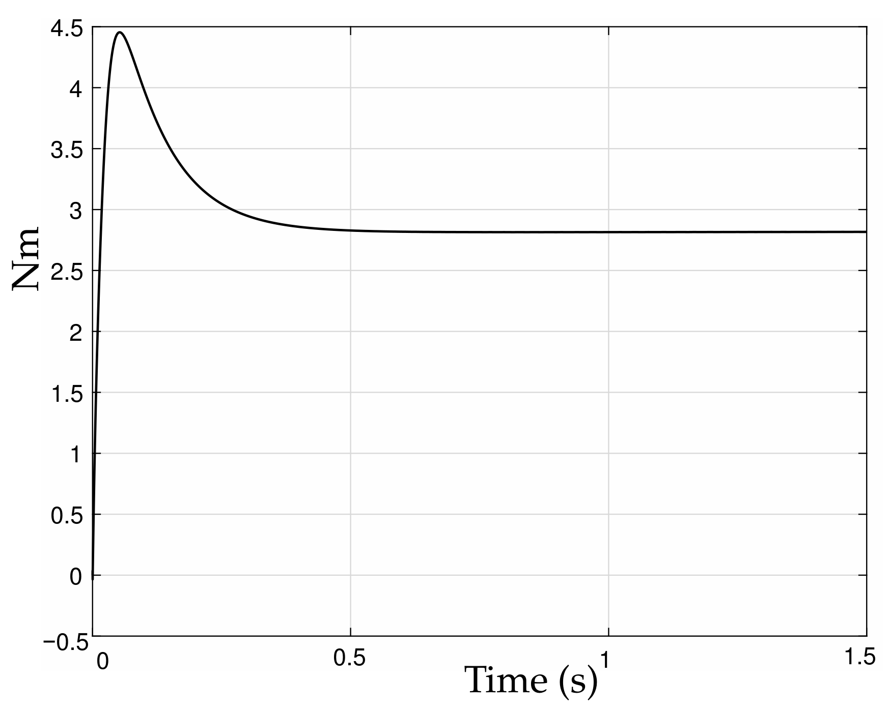
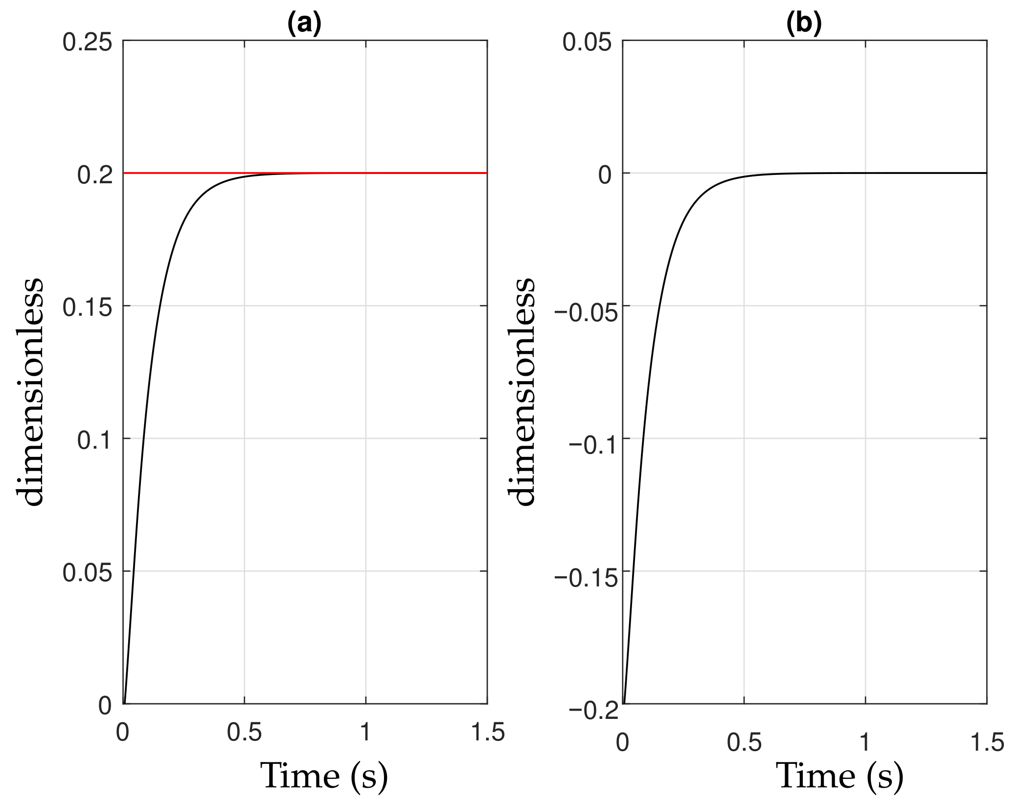
4.1. Numerical Simulation Result

In this subsection, some numerical simulations are shown to confirm the theoretical results. The simulations were performed with the modified HOSM controller using the PID-sliding surface (14) for the mathematical model of the ABS laboratory setup (5). These simulations showed an automobile running at a speed of $63.43$ km/h. For this particular scenario, the initial conditions of the ABS laboratory setup were ${\omega }_1\left(0\right)={\omega }_2\left(0\right)=180$ rad/s, i.e., $v_x\left(0\right)=r_2{\omega }_2\left(0\right)=17.62$ m/s, $v_w\left(0\right)=r_1{\omega }_1\left(0\right)=17.71$ m/s, and $T_b\left(0\right)=0$. The parameters and gains used in the ABS model (5) and the proposed controller (14) were those in Table 1 and

Table 2. Coefficients of controllers (14) and (26) used in the numerical and real-time simulations.

Symbol	Parameter	Value
${\gamma }_1$	Gain in modified HOSM	2.62
${\gamma }_2$	Gain in modified HOSM	0.9
${\gamma }_3$	Gain in modified HOSM	1.7
${\gamma }_4$	Gain in modified HOSM	10
$k_p$	PID-sliding surface	5.5
$k_i$	PID-sliding surface	20
$k_d$	PID-sliding surface	0.015
$k_{p,c}$	PID-like controller gain	32
$k_{i,c}$	PID-like controller gain	15
$k_{d,c}$	PID-like controller gain	15

, respectively. However, to test the controller robustness, the parameters used in the ABS model (5), i.e., the real ABS setup parameters, were augmented by 10% with respect to those in Table 1. The numerical simulation results are summarized in Figure 2, Figure 3 and Figure 4.

Figure 2 shows the control input applied in the simulator, and Figure 3 displays the angular velocity of the upper wheel ${\omega }_1$ and the angular velocity of the lower wheel ${\omega }_2$. Finally, Figure 4 presents the convergence of wheel slip $\lambda$ to its reference ${\lambda }_{\mathrm{ref}}=0.2$ in about $0.06$ s.

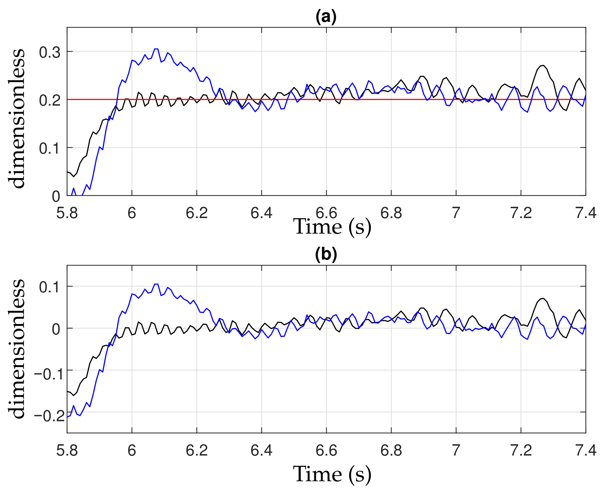
4.2. Experimental Result

In this subsection, the performance of the modified HOSM controller using a PID-sliding surface (14) applied to a real-time ABS laboratory setup is shown. Moreover, the real-time results obtained with the proposed controller (14) are compared with another controller available in the literature, the PID-like controller (26) proposed in [11,26,37]. The variables and the values of the ABS laboratory setup (5) are given in Table 1. Moreover, the parameters used in the controllers (14) and (26) are given in Table 1 and Table 2, respectively. To test the proposed controller robustness, a reader could consider that the coefficients in Table 1 may vary in practice due to natural wear for the mechatronic device but may remain close to these values.

Similar to the numerical simulations, the tests considered ${\omega }_1\left(0\right)={\omega }_2\left(0\right)=178$ rad/s (1700 RPM) and $T_b\left(0\right)=0$ as initial conditions for (5). These settings simulated a vehicle at a velocity of $63.43$ km/h, and the brake system is abruptly activated, sending a control input to the actuator to start a braking phase. It is worth remarking that for this setup, the nominal value of the friction coefficient between the two wheels used in (4) is given by the manufacturer as $\mu =1$.

The experimental results are summarized in Figure 5, Figure 6 and Figure 7, where the proposed controller, (14), ensures a better performance with respect to the PID-like controller, (26). Figure 5 shows the wheel velocity $v_w$ and the vehicle longitudinal velocity $v_x$. The wheel slip $\lambda$ and the tracking error $\lambda -{\lambda }_{\mathrm{ref}}$ are shown in Figure 6. The applied input $T_b$ is shown in Figure 7.

Analyzing Figure 7, we emphasize that controller (14) imposes higher control values than the PI-like controller (26). In this sense, the reduction in the braking time and space, as indicated in Figure 5, is quite natural. The latter could induce higher stress in the actuator. However, since the ABS is an emergency device that does not take any actions during normal braking but rather during only emergency braking, this aspect and the energy minimization are marginal.

After the braking process taking place at 5.5 and 7.4 s, corresponding to the peak braking efficiency, we highlight that the performance is no longer considered as the velocity is insignificant at this point and the ABS is not operating in the appropriate scope of velocities anymore. Figure 5 shows that both controllers maintain deceleration at a constant pace. The difference lies in the time that the controllers take to complete the braking phase; the proposed controller (14) manages to stop a few fractions of a second before the PID-like controller due to the proposed controller maintaining a $\lambda$ close to the reference, as shown in Figure 6, compared with the PID-like controller. After the braking phase, the reference tracking is pointless because the longitudinal velocity is too low and the ABS is rendered ineffective.

5. Conclusions

This work presented an analysis and the functionality of the design of a modified HOSM controller using a PID-sliding surface; this controller design was applied to the ABS laboratory setup. Numerical simulations were used to observe the performance of the proposed controller without parametric variations. Furthermore, a real-time simulation was applied to the ABS laboratory setup. These simulations were compared with a PID-like controller. Finally, the stability proof of a modified HOSM using a PID-sliding surface was verified. Future work will deal with a dynamic controller applied to the ABS, embedding an HOSM observer for the longitudinal velocity of a vehicle using information available from the laboratory setup. This controller will consider parametric uncertainties and the saturation problem of the mechatronic system.

References

1. Emelyanov, S.V.; Korovin, S.K.; Levantovsky, L.V. Higher order sliding regimes in the binary control systems. Doklady Akademii Nauk Russ. Acad. Sci. 1986, 287, 1338–1342. [Google Scholar]
2. Utkin, V.; Poznyak, A.; Orlov, Y.; Polyakov, A. Conventional and High Order Sliding Mode Control. J. Franklin Inst. 2020, 357, 10244–10261. [Google Scholar] [CrossRef]
3. Fridman, L.; Moreno, J.; Iriarte, R. Sliding Modes after the First Decade of the 21st Century: State of the Art; Lecture Notes in Control and Information Sciences; Springer: Berlin/Heidelberg, Germany, 2011; Volume 412, pp. 113–149. [Google Scholar]
4. Edwards, C.; Spurgeon, S.K. Sliding Mode Control: Theory and Application; Taylor and Francis Ltd.: London, UK, 1999. [Google Scholar]
5. Fridman, L.; Levant, A. Higher Order Sliding Modes. In Sliding Mode Control in Engineering; Perruquetti, W., Barbot, J.P., Eds.; CRC Press: New York, NY, USA, 2002; pp. 53–101. [Google Scholar]
6. Fridman, L.; Shtessel, Y.; Edwards, C.; Yan, X.G. Higher order sliding mode observer for state estimation and input reconstruction in nonlinear systems. Int. J. Robust Nonlinear Control 2008, 18, 399–413. [Google Scholar] [CrossRef]
7. Levant, A. Homogeneity approach to High–Order Sliding Mode design. Automatica 2005, 41, 823–830. [Google Scholar] [CrossRef]
8. Angulo, M.; Moreno, J.; Fridman, L. The differentiation error of noisy signals using the generalized super–twisting differentiator. In Proceedings of the 51st IEEE Conference on Decision and Control (CDC), Maui, HI, USA, 10–13 December 2012; pp. 7383–7388. [Google Scholar]
9. Liu, J.; Gao, L.; Zhang, J.; Yan, F. Super-twisting algorithm second-order sliding mode control for collision avoidance system based on active front steering and direct yaw moment control. Proc. Inst. Mech. Eng. Part D J. Autom. Eng. 2020, 235, 43–54. [Google Scholar] [CrossRef]
10. Zhang, L.; Ding, H.; Shi, J.; Huang, Y.; Chen, H. An Adaptive backstepping sliding mode controller to improve Vvehicle maneuverability and stability via torque vectoring control. IEEE Trans. Veh. Technol. 2020, 69, 2598–2612. [Google Scholar] [CrossRef]
11. Etienne, L.; Acosta-Lúa, C.; Di Gennaro, S.; Barbot, J.P. A super-twisting controller for active control of ground vehicles with lateral tire-road friction estimation and CarSim validation. Int. J. Control Autom. Syst. 2020, 18, 1177–1189. [Google Scholar] [CrossRef]
12. Cappelli, M.; Castillo-Toledo, B.; Di Gennaro, S. Nonlinear control of pressurized water reactors with uncertainties estimation via high order sliding mode. J. Franklin Inst. 2021, 358, 1308–1326. [Google Scholar] [CrossRef]
13. Gutiérrez-Oribio, D.; Mercado-Uribe, A.; Moreno, J.A.; Fridman, L. Reaction wheel pendulum control using fourth-order discontinuous integral algorithm. Int. J. Robust Nonlinear Control 2020, 31, 185–206. [Google Scholar] [CrossRef]
14. Blas, L.A.; Dávila, J.; Salazar, S.; Bonilla, M. Robust trajectory tracking for an uncertain UAV based on active disturbance rejection. IEEE Control Syst. Lett. 2022, 6, 1466–1471. [Google Scholar] [CrossRef]
15. Zhai, J.; Li, Z. Fast–exponential sliding mode control of robotic manipulator with super-twisting method. IEEE Trans. Circuits Syst. II Express Briefs 2022, 69, 489–493. [Google Scholar] [CrossRef]
16. Guo, X.G.; Ahn, C.K. Adaptive fault-tolerant pseudo PID sliding–mode control for high–speed train with integral quadratic constraints and actuator saturation. IEEE Trans. Intel. Transp. Syst. 2020, 22, 7421–7431. [Google Scholar] [CrossRef]
17. Zakia, U.; Moallem, M.; Menon, C. PID-SMC controller for a 2-DOF planar robot. In Proceedings of the International Conference on Electrical, Computer and Communication Engineering (ECCE), Cox’s Bazar, Bangladesh, 7–9 February 2019; pp. 1–5. [Google Scholar]
18. Gu, G.Y.; Li, C.X.; Zhu, L.M.; Fatikow, S. Robust tracking of nanopositioning stages using sliding mode control with a PID sliding surface. In Proceedings of the IEEE/ASME International Conference on Advanced Intelligent Mechatronics (AIM), Besacon, France, 8–11 July 2014; pp. 973–977. [Google Scholar]
19. Eker, I. Second–order sliding mode control with PI sliding surface and experimental application to an electromechanical plant. Arab. J. Sci. Eng. 2012, 37, 1969–1986. [Google Scholar] [CrossRef]
20. Khan, A.H.; Li, S. Sliding mode sontrol with PID sliding surface for active vibration damping of pneumatically actuated soft robots. IEEE Acces 2020, 8, 88793–88800. [Google Scholar] [CrossRef]
21. Navarrete-Guzmán, A.; Vaca-García, C.C.; Di Gennaro, S.; Acosta-Lúa, C. HOSM controller using PI sliding manifold for an integrated active control for wheeled vehicles. Math. Probl. Eng. 2021, 2021, 5482421. [Google Scholar]
22. Nilav-Aydina, M.; Cobanb, R. PID sliding surface-based adaptive dynamic second-order fault-tolerant sliding mode control design and experimental application to an electromechanical system. Int. J. Control 2020, 1–10. [Google Scholar] [CrossRef]
23. Kang, B.; Miao, Y.; Liu, F. A second-order sliding mode controller of quad–rotor UAV based on PID sliding mode surface with unbalanced load. J. Syst. Sci. Complex. 2021, 34, 520–536. [Google Scholar] [CrossRef]
24. ABS. The Laboratory Anti-Lock Braking System, User’s Manual; Inteco Ltd.: Krakow, Poland, 2006. [Google Scholar]
25. Al-Mola, M.H.; Mailah, M.; Samin, P.M.; Muhaimin, A.H.; Abdullah, M.Y. Performance comparison between sliding mode control and active force control for a nonlinear anti–lock brake system. WSEAS Trans. Syst. Control 2014, 9, 101–107. [Google Scholar]
26. Martinez-Gardea, M.; Mares Guzmán, I.J.; Di Gennaro, S.; Acosta Lúa, C. Experimental comparison of linear and nonlinear controllers applied to an antilock braking system. In Proceedings of the IEEE Conference on Control Applications (CCA), Juan Les Antibes, France, 8–10 October 2014; pp. 71–76. [Google Scholar]
27. Acosta-Lúa, C.; Di Gennaro, S.; Sánchez-Morales, M.E. An adaptive controller applied to an anti–lock braking system laboratory. Dyna 2016, 83, 69–77. [Google Scholar] [CrossRef]
28. Acosta–Lúa, C.; Di Gennaro, S.; Sanchez Morales, M.E. Nonlinear adaptive controller applied to an antilock braking system with parameters variations. Int. J. Control Autom. Syst. 2017, 15, 2043–2052. [Google Scholar] [CrossRef]
29. Precup, R.E.; Spataru, S.V.; Radac, M.B.; Petriu, E.M.; Preitl, S.; David, R.C. Experimental results of model–based fuzzy control solutions for a laboratory antilock braking system. In Human—Computer Systems Interaction: Backgrounds and Applications 2; Springer: Berlin/Heidelberg, Germany, 2012; pp. 223–234. [Google Scholar]
30. Radac, M.B.; Precup, R.E.; Preitl, S.; Tar, J.K.; Petriu, E.M. Linear and fuzzy control solutions for a laboratory anti–lock braking system. In Proceedings of the 6th IEEE International Symposium on Intelligent Systems and Informatics (SISY), Subotica, Serbia, 26–27 September 2008; pp. 26–27. [Google Scholar]
31. Khanesar, M.A.; Kayacan, E.; Teshnehlab, M.; Kaynak, O. Extended Kalman filter based learning algorithm for type–2 fuzzy logic systems and its experimental evaluation. IEEE Trans. Ind. Electron. 2012, 59, 4443–4455. [Google Scholar] [CrossRef]
32. Topalov, A.V.; Kayacan, E.; Oniz, Y.; Kaynak, O. Neuro–fuzzy control of antilock braking system using variable structure–systems based learning algorithm. In Proceedings of the International Conference on Adaptive and Intelligent Systems, Klagenfurt, Austria, 24–26 September 2009; pp. 1–6. [Google Scholar]
33. Martinez-Gardea, M.; Mares Guzmán, I.J.; Acosta Lúa, C.; Di Gennaro, S.; Vázquez Álvarez, I. Design of a nonlinear observer for a laboratory antilock braking system. J. Control Eng. Appl. Inf. 2015, 17, 105–112. [Google Scholar]
34. Acosta Lúa, C.; Di Gennaro, S.; Castillo-Toledo, B.; Martinez-Gardea, M. Dynamic control applied to a laboratory antilock braking system. Math. Probl. Eng. 2015, 2015, 896859. [Google Scholar] [CrossRef]
35. Martinez-Gardea, M.; Acosta-Lúa, C.; Vázquez-Álvarez, I.; Di Gennaro, S. Event–triggered linear control design for an antilock braking system. In Proceedings of the IEEE International Autumn Meeting on Power, Electronics and Computing (ROPEC), Ixtapa, Mexico, 4–6 November 2015; pp. 1–6. [Google Scholar]
36. Chereji, E.; Mircea-Bogdan, R.; Alexandra-Iulia, S.S. Sliding mode control algorithms for anti–lock braking systems with performance comparisons. Algorithms 2021, 14, 2. [Google Scholar] [CrossRef]
37. Acosta-Lúa, C.; Di Gennaro, S.; Barbot, J.P. Nonlinear control of an antilock braking system in the presence of tire–road friction uncertainties. J. Franklin Inst. 2022, 359, 2608–2626. [Google Scholar] [CrossRef]
38. Bosch, R. Bosch Automotive Handbook, 8th ed.; Wiley: Hoboken, NJ, USA, 2011. [Google Scholar]
39. Pacejka, H. Tyre and Vehicle Dynamics; Elsevier: Amsterdam, The Netherlands, 2006. [Google Scholar]
40. Ȧmströng, K.J.; Hägglund, T. PID Controllers: Theory, Design, and Tunning; ISA—The instrumentation, Systems, and Automation Society: Pittsburgh, PA, USA, 1995. [Google Scholar]
41. Moreno, J.A.; Osorio, M. A Lyapunov approach to second–order sliding mode controllers and observers. In Proceedings of the 47th IEEE Conference on Decision and Control, Cancun, Mexico, 9–11 December 2008; pp. 2856–2861. [Google Scholar]
42. Khalil, H.K. Nonlinear Systems, 3rd ed.; Prentice-Hall: Englewood Cliffs, NJ, USA, 2002. [Google Scholar]
43. Franklin, G.F.; Powell, J.D.; Emami-Naeini, A. Feedback Control of Dynamic Systems, 6th ed.; Pearson: New York, NY, USA, 2009. [Google Scholar]
Figure 1. The Inteco experimental setup and its scheme.
Applsci 12 03796 g001
Figure 2. Braking torque T b .
Applsci 12 03796 g002
Figure 3. Angular velocity of upper wheel ω 1 (solid) and angular velocity of lower wheel ω 2 (dashed).
Applsci 12 03796 g003
Figure 4. (a) Wheel slip λ (black) and reference λ ref (red); (b) tracking error λ λ ref .
Applsci 12 03796 g004
Figure 5. (a) Wheel velocity v w : a modified HOSM controller using PID-sliding surface (14) (black) or PID-like controller (26) (blue) and (b) vehicle longitudinal velocity v x : a modified HOSM controller using PID-sliding surface (14) (black) or PID-like controller (26) (blue).
Applsci 12 03796 g005
Figure 6. (a) Wheel slip λ : a modified HOSM controller using PID-sliding surface (14) (black), PID-like controller (26) (blue), or the reference λ ref (red) and (b) tracking error λ λ ref : a modified HOSM controller using PID-sliding surface controller (14) (black) or PID-like controller (26) (blue).
Applsci 12 03796 g006
Figure 7. Braking torque T b applied to the ABS laboratory setup: a modified HOSM controller using PID-sliding surface (14) (black) or PID-like controller (26) (blue).
Applsci 12 03796 g007