Abstract
Body mass index (BMI) plays a vital role in determining the health of middle-aged people, and a high BMI is associated with various chronic diseases. This study aims to identify important lifelog factors related to BMI. The sleep, gait, and body data of 47 middle-aged women and 71 middle-aged men were collected using smartwatches. Variables were derived to examine the relationships between these factors and BMI. The data were divided into groups according to height based on the definition of BMI as the most influential variable. The data were analyzed using regression and tree-based models: Ridge Regression, eXtreme Gradient Boosting (XGBoost), and Category Boosting (CatBoost). Moreover, the importance of the BMI variables was visualized and examined using the SHapley Additive Explanations Technique (SHAP). The results showed that total sleep time, average morning gait speed, and sleep efficiency significantly affected BMI. However, the variables with the most substantial effects differed among the height groups. This indicates that the factors most profoundly affecting BMI differ according to body characteristics, suggesting the possibility of developing efficient methods for personalized healthcare.
1. Introduction
A lifelog is an integrated digital record consisting of personal data collected from various digital sensors [1] such as activity, sleep information, weight change, body mass, muscle mass, and fat mass. With the development of wearable devices, more accurate and precise measurements are possible. Lifelog information obtained by wearable devices, such as gait, sleep, and weight, is now used for chronic disease occurrence monitoring and health care [2,3,4]. However, healthcare services using lifelogs are currently limited to simple records or incomplete statistics. Even if they include exercise and lifestyle feedback functions, the feedback provided is not personalized according to user characteristics. Therefore, this study aims to identify factors that can be used to develop personalized healthcare through lifelog analysis. This study interprets machine learning results using an interpretable model rather than a black box model.
Most previous studies on the correlation between BMI and weight with disease incidence have used medical data [5,6]. In contrast, we used lifelogs of sleep, steps, and weight in daily life. Individual analysis was subsequently performed using machine learning algorithms.
The rest of this paper is organized as follows. Section 2 describes the use and importance of lifelog data. Section 3 analyzes the association between lifelog data and BMI using regression machine learning algorithms. Section 4 details the method used, and Section 5 compares the results with prior research and relevant references.
2. Importance of Lifelog Analysis: Relationship between Lifelog and Diseases
2.1. Relationship between Walking and Disease
According to the U.S. Physical Activity Guidelines [7] and the U.K. Public Health Agency [8], walking can be easily achieved by anyone in their daily and work lives to help prevent cardiovascular and other diseases. According to a cohort study involving menopausal women, walking significantly reduced the risk of developing cardiovascular disease [9]. Moreover, among 10 cohort studies, five studies on walking showed that individuals who did the most walking had a significantly lower risk of type 2 diabetes than those who performed the least walking [10]. In addition, a study of men below and above the age of 62 showed that a 3 min walk every 30 min helped to control blood sugar [11].
2.2. Relationship between Sleep and Disease
Sleep is essential for maintaining good health. Adults who do not sleep for 7–8 h regularly have a higher risk of cardiovascular disease, diabetes, obesity, and mortality [5]. A previous study found that the risk of hypertension increased as sleep time decreased [12]. Body mass index (BMI) is also closely related to sleep. Sleeping for less than five hours has increased the risk of obesity by 1.5 times, with BMI increasing by 0.35 kg/m2 for every one-hour decrease in sleep time [13]. Some studies have shown that even more than eight hours of sleep are associated with increased BMI and obesity [14,15]. Moreover, the risk of type 2 diabetes has increased with less than six hours [16] and even with more than nine hours of sleep [17]. Previous studies have also shown that sleep time correlates with cancer incidence, with short sleep times increasing the risk of breast, colon, and prostate cancer [18,19,20,21]. The risk of developing breast cancer is lower in women who sleep for more than nine hours [22]. Furthermore, epidemiological studies have shown that nightshift workers have an increased risk of developing breast, colon, prostate, and endometrial cancer [23,24].
2.3. Relationship between Weight and Disease
Weight gain is known to be associated with an increased risk of type 2 diabetes, coronary artery disease, high blood pressure [25], cholelithiasis [26], and several cancers [27]. A study that used cohort survey data from 92,837 women and 25,303 men in the U.S. to investigate how weight changes from adolescence to middle age are associated with various chronic diseases after the age of 55 years found that weight gain increased the risk of type 2 diabetes, hypertension, cardiovascular disease, obesity-related cancer, cholelithiasis, severe osteoarthritis, and cataracts.
In this study, weight was used as an indicator of health status; sleep and gait were used as independent variables related to weight. However, as each person’s physical characteristics are unique, BMI was calculated and used as the response variable instead of weight.
3. The Association between Lifelog Data and BMI Using Regression Machine Learning Algorithms
Existing relevant studies can generally be categorized as follows.
3.1. Digital Healthcare Research Using Machine Learning and Data Generated by Smartphones and Smartwatches
One study proposed developing a severity score for Parkinson’s disease using smartphone sensor data and machine learning, which can provide helpful information for the clinical management and treatment of patients with the disease [28]. Other studies have proposed a motion recognition model related to the user’s meal intake using a smartwatch sensor [29].
3.2. Research on Men and Women’s Health Using Machine Learning
One study proposed a predictive model using individual health data that affects the mortality rate in women with breast cancer [30]; another study developed and tested an early prediction model that could predict diabetes in women with an accuracy of 81.1% using a factor analysis that was highly correlated with diabetes [31]. Other studies have used machine learning predictive models to identify women at high risk of postpartum depression [32].
3.3. Research on Weight and Weight Change Using Machine Learning
In a study that summarized the risk factors for obesity and overweight using machine learning, age and gender were selected as significant relevant risk factor variables [33]. In addition, some studies have classified and predicted high, medium, and low weight loss potential levels using machine learning algorithms and the dietary and exercise data of obese patients [34].
4. Methods
4.1. Data Collection
Data on sleep, gait, and weight of 47 women and 71 men aged 35–59 years were obtained using the GiVita Inc. app on Samsung Galaxy Watch Active2 smartwatches, collected from 1 February to 9 August 2021. The age was set at 35 to 59; we targeted middle age because the age at which health care begins is the age at which interest in health care is greatest.
We collected the data for these six months because the app was updated compared to the previous version, improving usability, stabilizing data, and reducing missing and abnormal values. First, updating the app resulted in fewer errors, making data collection more stable. Second, the user experience was significantly improved and rewards were provided as an update. The data included the users’ bedtimes, wake-up times, steps per minute and day, walking distance per minute and day, walking speed per minute and day, and daily weight. Based on these records, data on daily sleep in minutes, daily steps in minutes, and daily weight were created. The dataset sizes were 6223 rows of sleep data collected by day, 241,068 rows of sleep data collected by minute, 1,797,590 rows of step data collected per day, 6380 rows of step data collected by minute, and 6729 rows of body weight data collected by day.
4.2. Data Preprocessing
To find the optimal variables explaining individual BMI variance, several variables, such as total daily sleep time and sleep efficiency, were generated using daily sleep data and sleep data in minutes. Likewise, derivative variables, such as the total number of steps per day and average walking speed in the morning, were generated using the daily step data and step data in minutes. Additionally, the users’ body data, such as height and weight, were integrated with each day’s step and sleep data. The derivative variables are shown in Appendix A: Table A1.
4.3. Feature Selection
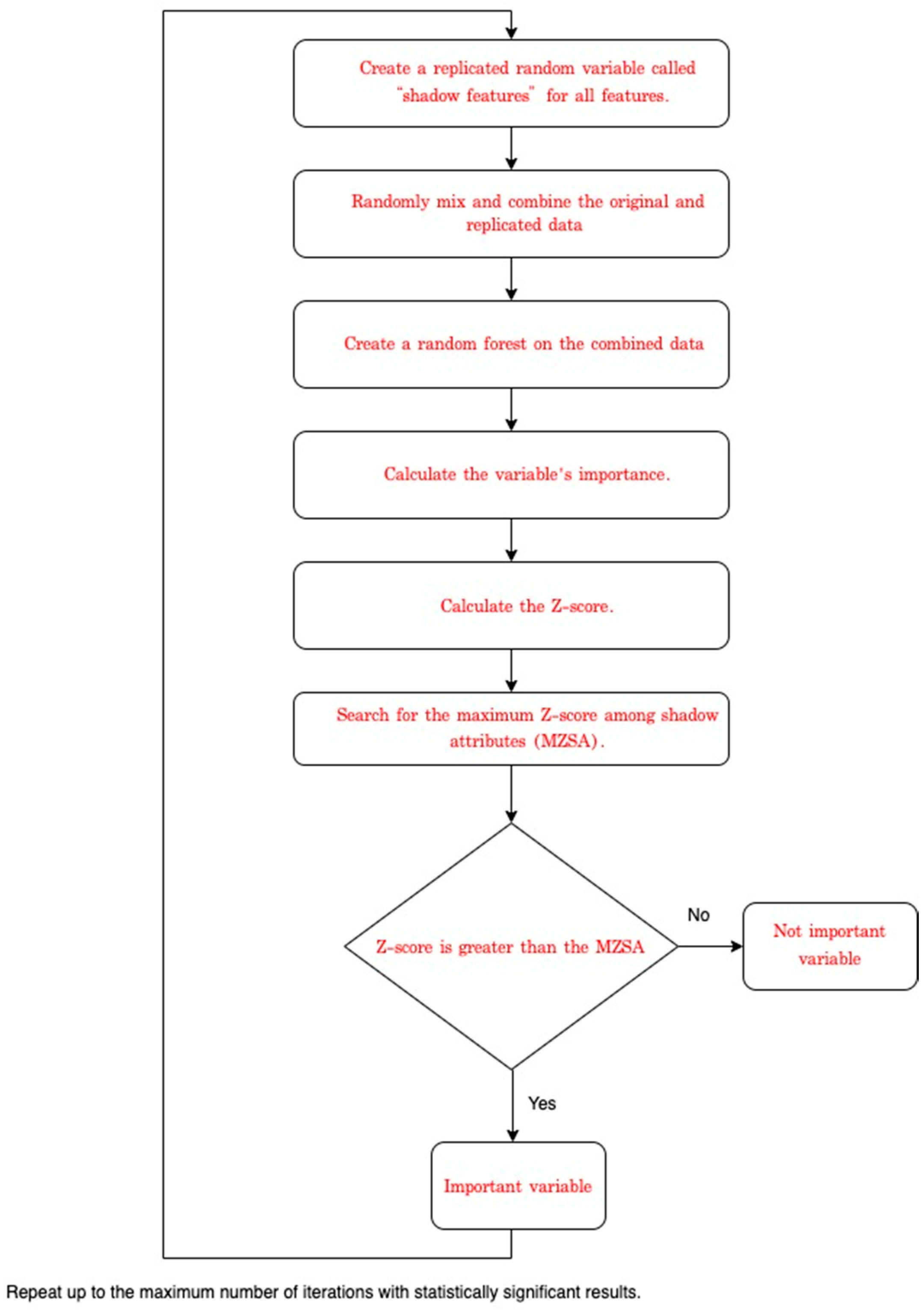
If all 55 derived variables (Table A1) were used as inputs in the model, there would be a risk of overfitting. Therefore, feature selection was performed to remove unnecessary variables. This study selected features using the Boruta SHapley Additive exPlanations (BorutaSHAP) method, which combines the Boruta feature selection algorithm with SHAP values [35]. The execution procedure of the Boruta algorithm can be summarized as follows [36], and Figure 1 shows the procedure of Boruta feature selection.

Figure 1.
Flow chart of procedure of the Boruta feature selection.
- Create a replicated random variable called “shadow features” for all features.
- Randomly mix and combine the original and replicated data to remove possible correlations between dependent variables and features.
- Create a random forest on the combined data and calculate the variable’s importance.
- Calculate the Z-score.
- Search for the maximum Z-score among shadow attributes (MZSA).
- For raw data, if the Z-score is greater than the MZSA, it is an important variable.
- Repeat the above process as often as the random forest is performed, or until each variable is marked as either important or non-significant.
In previous studies, algorithm experiments on multiple datasets have shown that the Boruta method is better at feature selection than the Chi-Square method [37]. Boruta is a method of selecting variables based on a random forest. In addition, the BorutaSHAP process uses the Light Gradient Boosting Machine (LGBM), Category Boosting (CatBoost) (which robustly addresses categorical variables, as well as random forests), or other boosting-type models, such as eXtreme Gradient Boosting (XGBoost), to calculate feature importance. BorutaSHAP provides flexibility in model selection and allows visualization of the selected features by applying the SHAP [35].
Therefore, the BorutaSHAP algorithm was used in this study for flexible model selection and convenient visualization of the key selected variables. This method extracts important features using thresholds and t-tests on data with random shadow variables added.
As there are few categorical variables in this study, and the feature importance computed using random forest can be biased in some cases [38], to calculate the feature importance, the XGBoost model was selected instead [39]. The strengths of the BorutaSHAP algorithm are the consistency of feature importance [40] and the use of intuitive colors to visualize the feature importance.
As shown in Figure 2, most of the sleep variables in the variable list extracted using BorutaSHAP, except for the total number of hours of sleep per day, are in red and do not significantly influence the generation of rules related to BMI prediction. These steps can directly affect BMI. Most of the variables are green and can be identified as primary variables. In addition, height, which is very closely related to BMI, was also identified as a significant variable. The four blue boxes represent the minimum, median, mean, and maximum attributes. The yellow box means tentative, the importance of which is difficult to determine. The reason is that this corresponding provisional attribute appears near the maximum attribute, which is challenging to identify in the basic random forest execution of the Boruta algorithm.
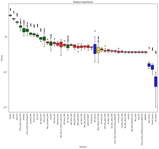
Figure 2.
Importance of variables calculated using the BorutaSHAP algorithm.
Figure 2 shows the feature importance obtained by the BorutaSHAP method for all data. The following features were selected: AVG_SPD, DIST_STD, DISTANCE, LNC_AVG_SPD, TOTAL_SLEEP_TIME_HOUR, STEP_COUNT, CALORIE, NT_AVG_SPD, LNC_WALK_DIST, NT_WALK_TIME, TOTAL_SLEEP_TIME_VARIABILITY, HEIGHT, and STEP_STD.
4.4. Data Modeling
The final features obtained using BorutaSHAP were learned using three models: XGBoost, CatBoost, and Ridge Regression. Table 1 shows the hyperparameters found by GridSearchCV in the Scikit-Learn (Sklearn) library and used in the three models. Training and test data were divided 8:2, and a 5-fold cross-validation was used for more accurate verification.

Table 1.
Hyperparameters for XGBoost, CatBoost, and Ridge Regression.
In this study, data were not normalized to remove outliers from data preprocessing and to facilitate the interpretation of the study results. Thus, we used ridge regression and tree-based machine learning models, such as XGBoost and CatBoost, which can operate relatively robustly without regularization.
4.5. Evaluation
This study mainly used five evaluation indicators: Explained Variance Score, R-squared score, adjusted-R-squared score, Mean Absolute Error (MAE), and Root Mean Squared Error (RMSE).
The description and calculation formulas of the performance indicators for each are as follows:
, , is the actual value, is the predicted value, and is the average of the actual values.
where is the number of samples and is the number of explanatory variables.
The Explained Variance Score is 1—((Sum of Squared Residuals—Mean Error)/Total Variance). The only difference between the Explained Variance Score (EVS) and the R-squared score is that the R-squared score subtracts the mean error from the Sum of Squared Residual (SSR). If the mean error is not close to zero, and a negative or positive value is obtained, the error is biased to one side and, thus, the model is biased. In other words, if the R-squared and the explanatory variance score are different, the error is biased, and there is a high possibility of incorrect fitting.
Compared to MAE, RMSE has the advantage of giving a sizable penalty for a significant error value difference and is strong.
5. Results
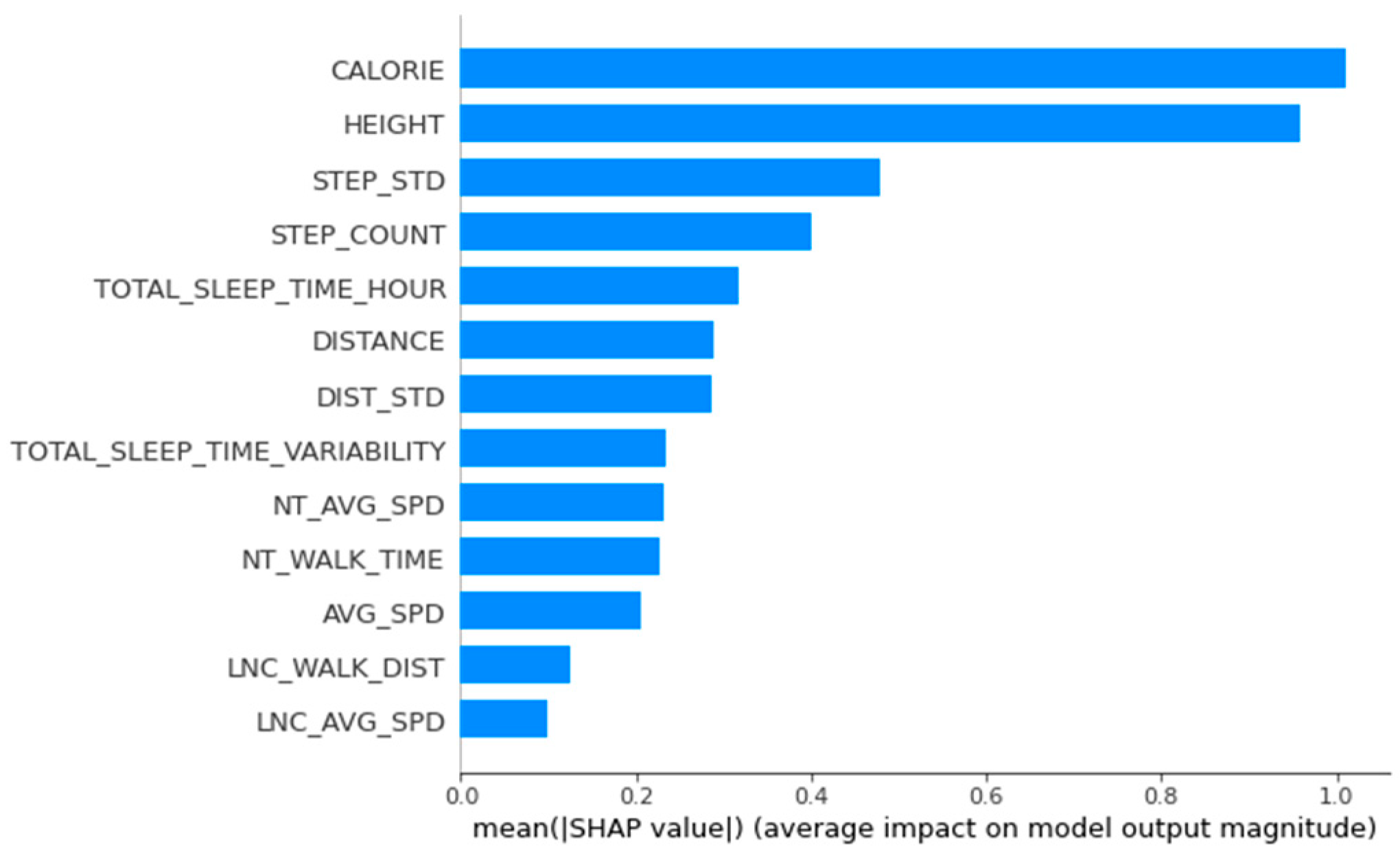
This study made predictions on the test dataset using a model based on the entire training data. The BMI values predicted by the model were analyzed using SHAP. Figure 2 shows the feature importance in XGBoost model using SHAP, which indicates that height is a highly importance feature. However, according to the BMI calculation formula, height already had a high correlation with BMI, regardless of model performance. It may not be possible to measure the influence of other variables correctly. Therefore, a clustering method was used to divide the data according to height, and the relationships between the variables and BMI were examined in each height group.
The reason for dividing the groups based on height was to accurately identify the degree of influence of the changeable activity variable on the BMI of users in the same group, as height is an immutable variable. According to the National Statistical Office of Korea and previous studies, the average heights of women in their 30s, 40s, and 50s in Korea are 161.59, 159.91, and 157.23 cm, respectively; the average heights of men in their 30s, 40s, and 50s in Korea are 174.05, 172.15, and 169.39 cm, respectively [41,42]. Figure 3 also shows that height was an important feature. Based on height, we divided the women’s data into two groups, 150–160 cm and 160–170 cm, and the men’s data into three groups, 165–170 cm, 170–175 cm, and 175–180 cm. To reduce the imbalance in the data due to excessive grouping, we divided the men’s data by 5 cm. For females, we formed two groups because the amount of data in a given group became too small when divided by 5 cm, resulting in performance problems.
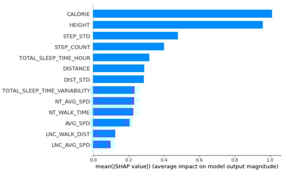
Figure 3.
Importance of variables calculated using SHapley Additive exPlanations.
Table 2 and Table 3 summarize the performance indicators of the three models in each cluster for men and women, respectively.
Table 2.
Comparison of the Performance Indicators of the XGBoost, CatBoost, and Ridge Regression Machine Learning Algorithms for each height group.
Table 3.
Comparison of the performance indicators of the XGBoost machine learning algorithms for each height group.
For modeling women’s data, it was decided to use only XGBoost based on the men’s data analysis results. The XGBoost algorithm is generally similar to or superior to Ridge Regression and CatBoost algorithms. The benefits of using CatBoost are limited because the features used for analysis have few categorical features.
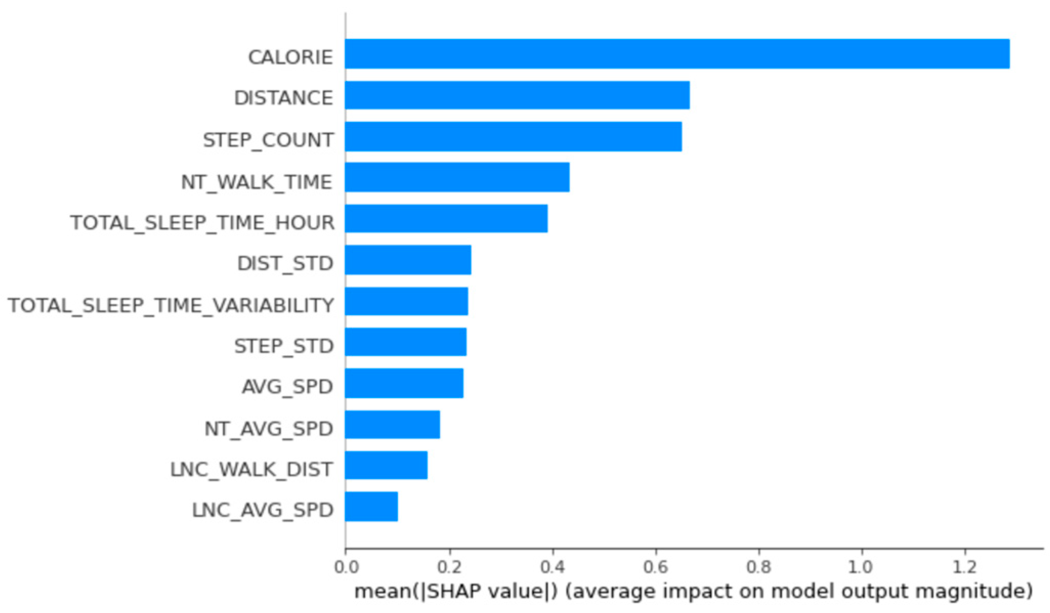
The main relevant variables for women’s group 1 were calories burned, distance, number of steps, time walked at night, and total sleep time per day (Figure 4).

Figure 4.
Feature importance calculated using the SHapley Additive exPlanations for women’s group 1.
A figure illustrating the data of women’s group 2 can be found in the Appendix A (Figure A1). The main variables of women’s group 2 were calories burned by walking, total sleep time per day, total sleep time variability, gait variability, and average walking speed at night.
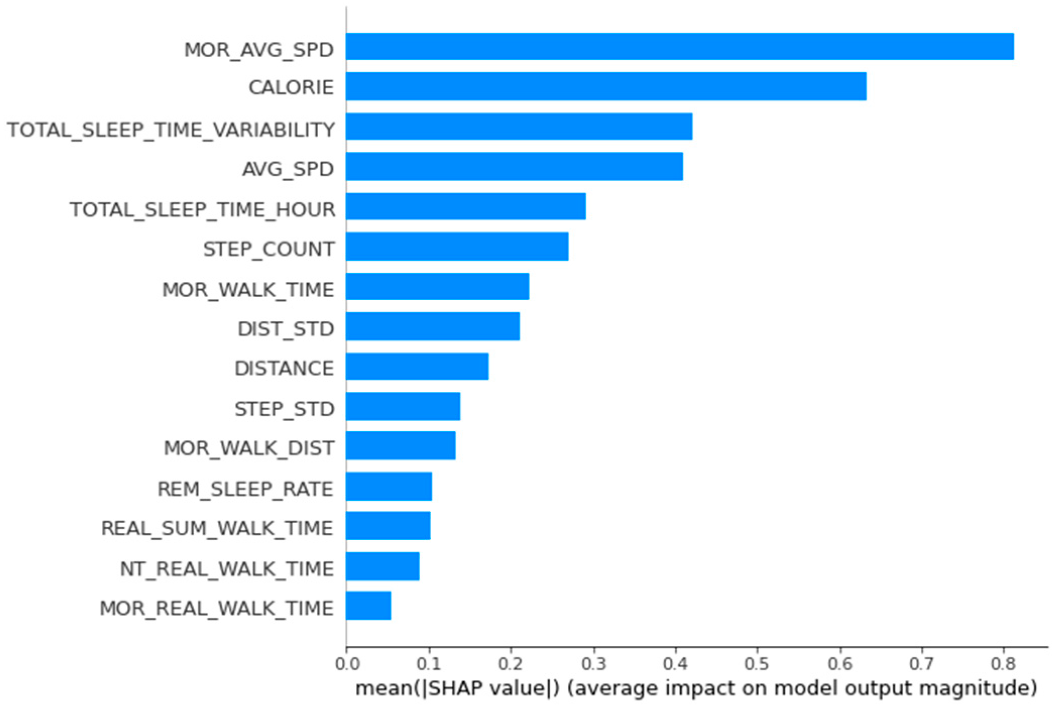
The men’s data were analyzed in the same way. The main variables of men’s group 1 were average morning walking speed, calories burned, total sleep time variability, daily average walking speed, and daily total sleep time. Considering the accumulated SHAP values for this group, we found that average walking speed in the morning based on the approximate distance lowered BMI and that total sleep time influenced increases in BMI (Figure 5).
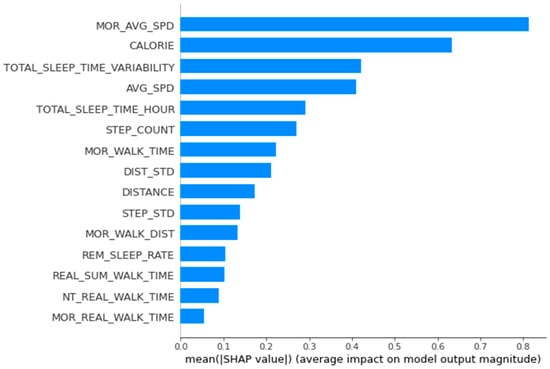
Figure 5.
Feature importance calculated using the SHapley Additive exPlanations for men’s group 1.
Figures illustrating the data from men’s groups 2 and 3 are presented in the Appendix A (Figure A2 and Figure A3). As for the main variables of men’s group 2, calories burned, distance walked, and the number of steps generally influenced whether BMI would be lower, as confirmed by the accumulated SHAP values of the group. The primary relevant variables of men’s group 3 were step variability, calorie consumption by walking, daily average walking speed, length of time spent walking at night, and walking distance variability. The accumulated SHAP values of the group confirmed that variability in the number of steps, distance walked, and amount of time walked at night influenced lowering BMI, and calorie consumption by walking influenced increasing BMI.
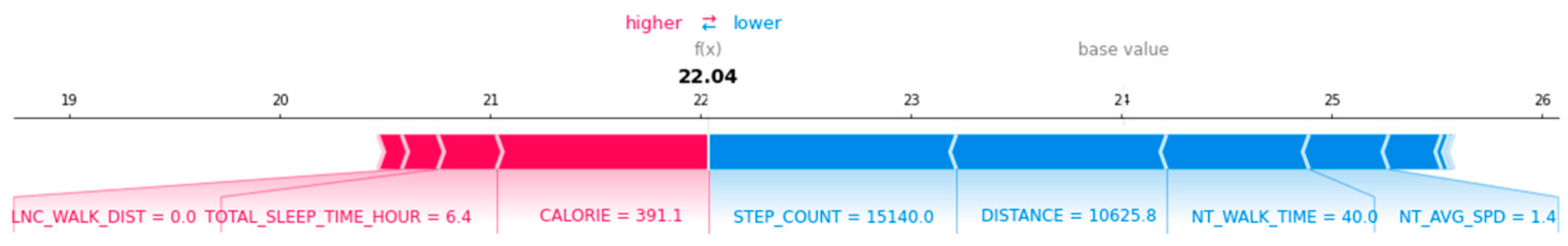
For the local interpretation of arbitrary data, the SHAP force plot was used. For the women in group 1, the number of steps, distance walked, amount of time walking at night, and average walking speed at night influenced lowering BMI. In contrast, calories and total sleep time affected increasing BMI (Figure 6).

Figure 6.
Local interpretation of arbitrary data in women’s group 1 using SHAP.
Figure A4 in the Appendix A summarizes the data on women’s group 2. In this group, the number of calories consumed, total sleep time, bedtime, step variability, and average speed walking at night affected a reduction in BMI. In contrast, total sleep time variability and average walking speed increased BMI.
Similarly, men’s group 1 data showed that step variability, total sleep time, average morning walking speed, and overall daily average walking speed affected a reduction in BMI. In contrast, variability in the length of time spent walking in the morning and total sleep time affected increasing BMI (Figure 7).
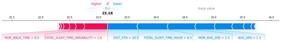
Figure 7.
Local interpretation of arbitrary data in men’s group 1 using SHAP.
Figures illustrating the data from men’s groups 2 and 3 can be found in the Appendix A (Figure A5 and Figure A6). An interpretation of the data for men’s group 2 showed that calorie consumption, number of steps walked per day, and distance walked affected a reduction in BMI. Step variability and distance walked in the morning affected the increase in BMI. For men’s group 3, the number of steps walked per day, step variability, step calorie consumption through walking, and amount of time walking at night affected a reduction in BMI. In contrast, total sleep time affected the increase in BMI.
6. Discussion
This study aims to identify the lifelog variable with the most decisive influence on BMI, closely related to health, by utilizing changeable gait and sleep lifelogs. The variables related to increases or decreases in BMI were also analyzed and specified.
Although lifelog data have recently been collected more efficiently and constantly by wearable devices, there are still limitations in the accuracy and quality of sleep data. Data collection can be unstable due to various external factors, such as battery and Wi-Fi communication. In addition, the accuracy of the data can be low because it is difficult for users to wear the devices continuously.
To improve the quality of sleep data, the study attempted to complement the limitations in accuracy by minimizing bias and anomalies. Various preprocessing and derivative variables such as total daily sleep time, variability in sleep time compared to the previous day, and daily sleep efficiency were generated. Further complementary research on sleep and accurate data collection and preprocessing of lifelogs is needed.
To determine the influence of each variable more accurately on BMI, we divided the data into two groups of women and three groups of men, and we compared the data using the representative machine learning regression models Ridge Regression, XGBoost, and CatBoost. We also used the highly effective SHAP method for explainable artificial intelligence to visualize the relative importance of variables to BMI changes. The predicted results were interpreted by combining the machine learning model and SHAP. In the case of a deep learning model, also known as a black box model, the performance of the prediction can be high, but the interpretation can be difficult.
Therefore, a SHAP-based interpretable machine learning model was used in this study. The advantages over the black box model include the following:
- Improved confidence in the machine learning model, providing a clear explanation of the results of the inference path.
- Deriving insights by interpreting the results: extracting associations and patterns.
- Improving overall problem solving and eliminating bias errors: debugging the way predictions are performed can increase predictive power, and the cause of bias can be analyzed and improved.
The integrated lifelog data analysis of walking, sleep, and weight with machine learning revealed the key variables and how walking and sleep affect body weight. For middle-aged individuals, lifelogs can inform specifically and individually tailored health analyses beyond simple predictions, and they can influence weight regulation through interpretable techniques and visualization.
In this study, the most common influential variables were calories burned, number of steps per day, distance walked per day, and sleep quality. These findings are consistent with those of previous studies, indicating that the number of steps [43], walking speed [44,45], and sleep quality [46,47] affect BMI.
The analysis highlights daily calorie consumption as an essential variable for predicting BMI. In the case of women’s group 1 (150–160 cm), calories burned per day, the number of steps per day, distance walked per day, and amount of time walking at night had the most significant effect on BMI. In women’s group 2 (160–170 cm), daily calorie consumption by walking, total sleep time, total sleep time variability, and step variability had the highest impact on BMI.
For men’s group 1 (165–170 cm), average morning walking speed, calorie consumption per day, and total sleep variability had the most substantial effects on BMI. In men’s group 2 (170–175 cm), calories burned per day, distance walked per day, and the number of steps per day had the greatest impact on BMI. Finally, in the case of men’s group 3 (175–180 cm), gait variability, calorie consumption per day, and average walking speed had the most significant effects on BMI.
Thus, factors such as height, diet, physical activity may affect physical changes and the incidence of diseases in different ways [48,49,50]. In addition, the effects of training methods may vary according to BMI and weight (body type) [51,52]. Experiments have found that different variables, including walking variables, may affect each group differently.
These findings provide evidence that the factors with the most decisive influence on BMI depend on the height and lifelog of an individual, suggesting the possibility of developing an efficient method for personalized healthcare in the future. Although this study has proposed various sleep and gait variables that affect BMI, it would be valuable for a follow-up study to determine specific values or ranges for each variable to support a healthy BMI.
Author Contributions
Conceptualization, J.K. and M.P.; data curation, J.K.; formal analysis, J.K.; funding acquisition, M.P.; methodology, J.K. and M.P.; supervision, M.P.; validation, J.K.; visualization, J.K.; writing—original draft preparation, J.K. and M.P.; and writing—review and editing, J.L. and M.P. All authors have read and agreed to the published version of the manuscript.
Funding
This work was supported by a research grant from Seoul Women’s University (2021-0423).
Institutional Review Board Statement
Not applicable.
Informed Consent Statement
Informed consent was obtained from all subjects involved in the study.
Conflicts of Interest
The authors declare no conflict of interest.
Appendix A
Table A1.
Description of Variables and Derived Variables.
Table A1.
Description of Variables and Derived Variables.
| Name of Variables | Description |
|---|---|
| AFT_AVG_SPD | Average walking speed in the afternoon (4:00 p.m.–8:00 p.m.) per day |
| AFT_REAL_WALK_TIME | The total length of time spent walking in the afternoon calculated based on the distance |
| AFT_WALK_DIST | Distance walked in the afternoon per day |
| AFT_WALK_TIME | The total length of time spent walking in the afternoon calculated by a Samsung Galaxy Watch |
| AGE | Age of user |
| AGE_CATEGORY_10 | Age group categorized in 10 years |
| AGE_CATEGORY_5 | Age group categorized in 5 years |
| AVG_SPD | Average walking speed per day |
| BED_TIME | Time when going to sleep |
| BED_TIME_AT_10PM_TO_12PM_FLAG | Whether BED_TIME is between 10:00 p.m. and 00:00 a.m. |
| BED_TIME_VARIANCE | The change in BED_TIME compared to the previous day |
| BED_TIME_VARIANCE_FLAG | Whether BED_TIME_VARIANCE is less than 2 h |
| BMI | BMI measured by a scale |
| BMI_INDEX | Category by BMI |
| BMI_STATUS | Weight status using BMI (underweight, normal, overweight, or obese) |
| CALORIE | Calorie consumption per day |
| DATE | Date |
| DEEP_SLEEP_RATE | Deep sleep (N3 sleep) ratio |
| DIST_STD | Standard deviation of distance walked per day |
| DISTANCE | Distance walked per day |
| FAT | Fat mass measured by a scale |
| GENDER | Gender of user |
| HEIGHT | Height of user |
| HEIGHT_CATEGORIZE_10 | Height group categorized in 10 cm |
| HEIGHT_CATEGORIZE_5 | Height group categorized in 5 cm |
| HOLIDAY | Whether it is a holiday or not |
| LNC_AVG_SPD | Average walking speed during lunchtime (11:00 a.m.–3:00 p.m.) per day |
| LNC_REAL_WALK_TIME | The total length of time spent walking in lunchtime calculated based on the distance |
| LNC_WALK_DIST | Distance walked during lunchtime per day |
| LNC_WALK_TIME | The total length of time spent walking during lunchtime calculated by a Samsung Galaxy Watch |
| MOR_AVG_SPD | Average walking speed in the morning(6:00 a.m.–10:00 a.m.) per day |
| MOR_REAL_WALK_TIME | The total length of time spent walking in the morning calculated based on the distance |
| MOR_WALK_DIST | Distance walked in the morning per day |
| MOR_WALK_TIME | The total length of time spent walking in the morning calculated by a Samsung Galaxy Watch |
| MUSCLE | Muscle mass measured by a scale |
| NAP_COUNT | Number of naps in a day |
| NT_AVG_SPD | Average walking speed at night (8:00 p.m.–00:00 a.m.) per day |
| NT_REAL_WALK_TIME | The total length of time spent walking at night calculated based on the distance |
| NT_WALK_DIST | Walked distance at night per day |
| NT_WALK_TIME | The total length of time spent walking at night calculated by a Samsung Galaxy Watch |
| REAL_SUM_WALK_TIME | The total daily walking time calculated based on the distance |
| REM_SLEEP_RATE | REM sleep ratio |
| SLEEP_EFFICIENCY | Sleep efficiency (the number of hours of sleep without waking up during sleep) |
| SPD_STD | Standard deviation of average walking speed per day |
| STEP_COUNT | Number of steps per day |
| STEP_STD | Standard deviation of number of steps per day |
| SUM_WALK_TIME | The total daily walking time calculated by a Samsung Galaxy Watch |
| TOTAL_COUNT_CONTINUOUS_WALK_20MINUTES | The total number of continuous walks for more than 20 min in a day |
| TOTAL_SLEEP_TIME_HOUR | Total number of hours of sleep per night |
| TOTAL_SLEEP_TIME_VARIABILITY | Standard deviation of the total number of hours of sleep per night |
| TOTAL_TIME_CONTINUOUS_WALK_20MINUTES | The total time of walking continuously for more than 20 min in a day |
| USER_CODE | Distinct user code |
| WEEKDAY | Day of the week other than Saturday or Sunday |
| WEEKEND | Whether it is the weekend or not |
| WEIGHT | Weight measured by a scale |
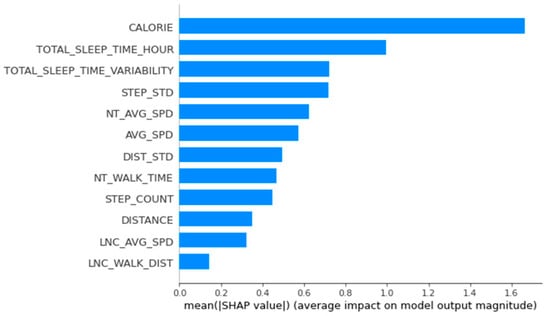
Figure A1.
Importance of variables calculated using the SHapley Additional exPlanations for women’s group 2.
Figure A1.
Importance of variables calculated using the SHapley Additional exPlanations for women’s group 2.
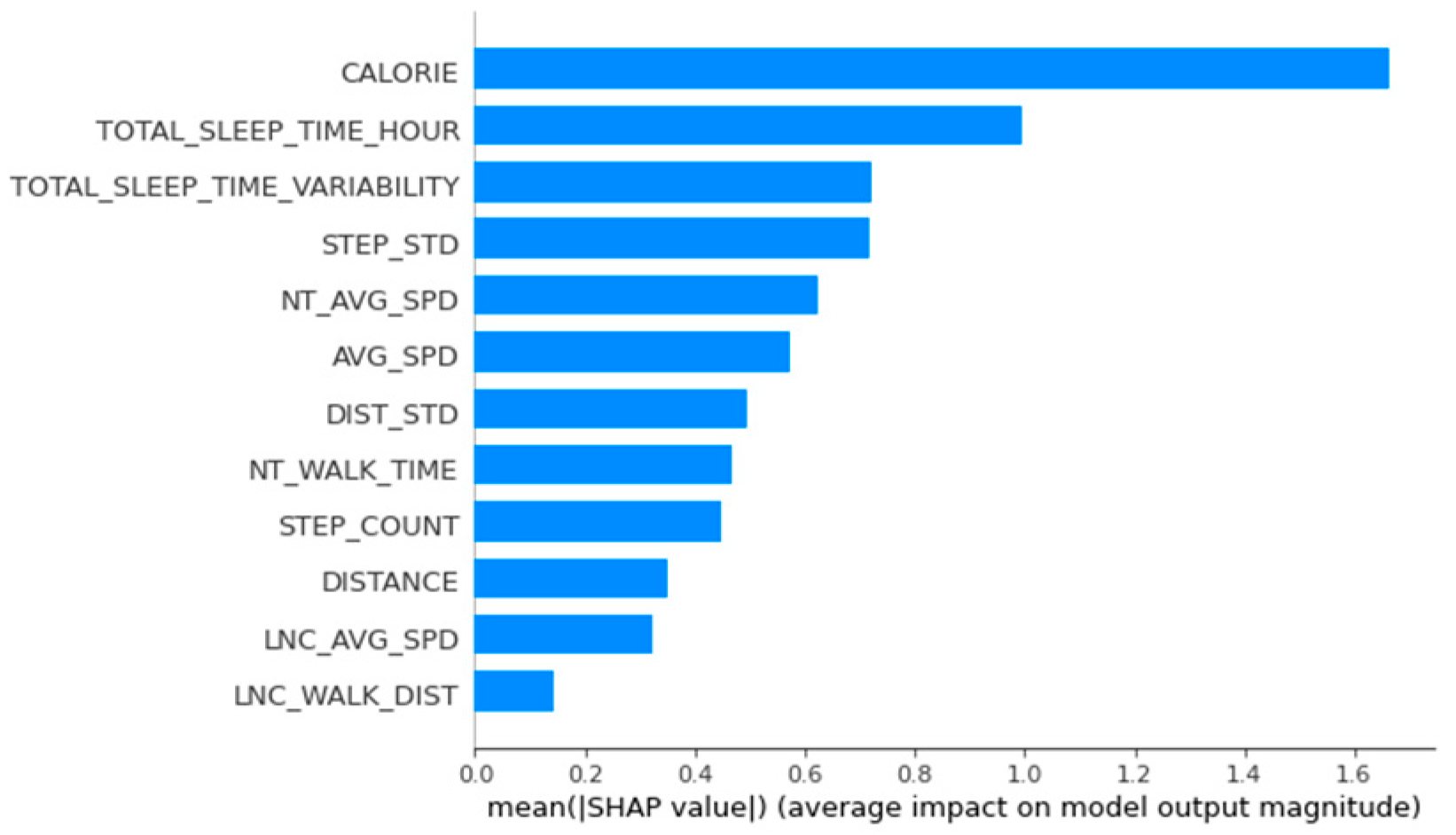

Figure A2.
Importance of variables calculated using the SHapley Additional exPlanations for men’s group 2.
Figure A2.
Importance of variables calculated using the SHapley Additional exPlanations for men’s group 2.
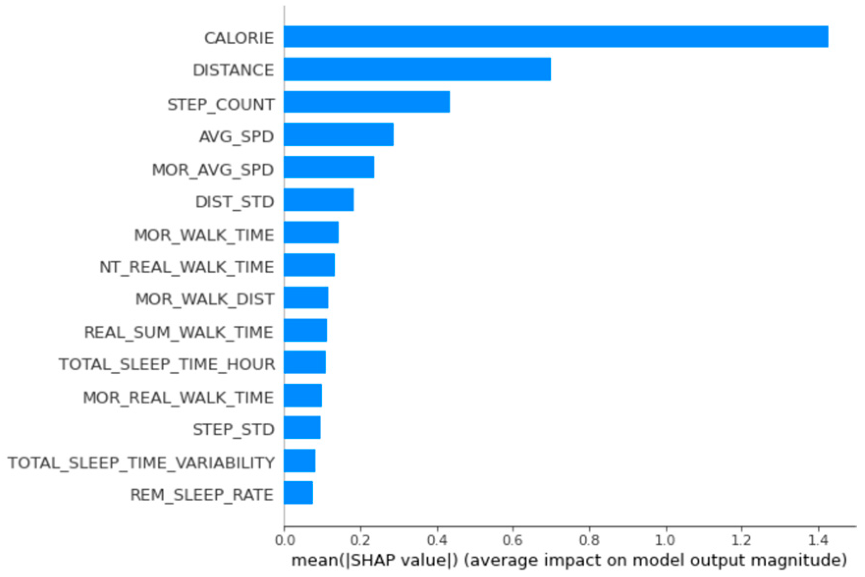
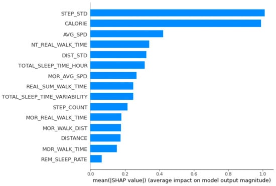
Figure A3.
Importance of variables calculated using the SHapley Additional exPlanations for men’s group 3.
Figure A3.
Importance of variables calculated using the SHapley Additional exPlanations for men’s group 3.
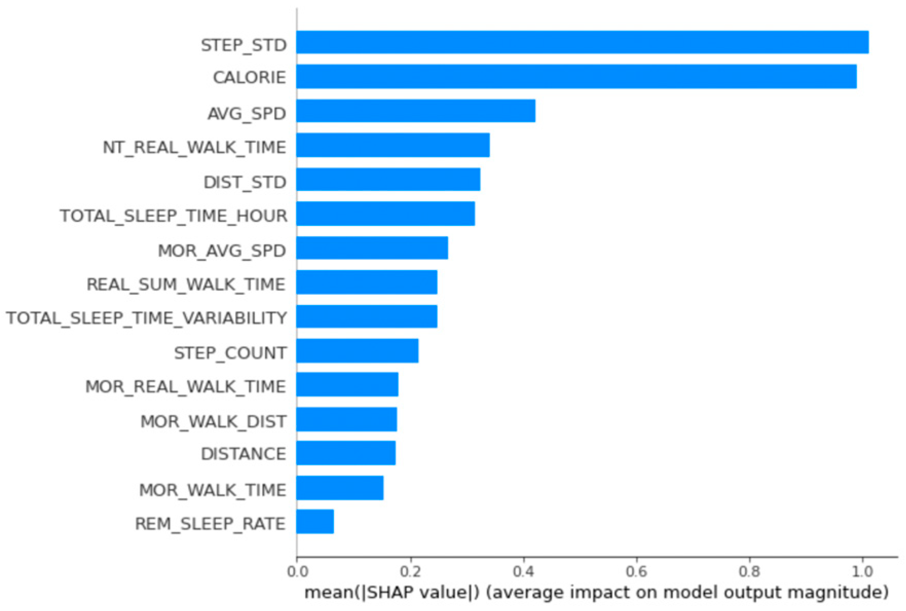
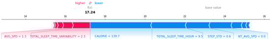
Figure A4.
Local interpretation of arbitrary data in women’s group 2 using SHAP.
Figure A4.
Local interpretation of arbitrary data in women’s group 2 using SHAP.
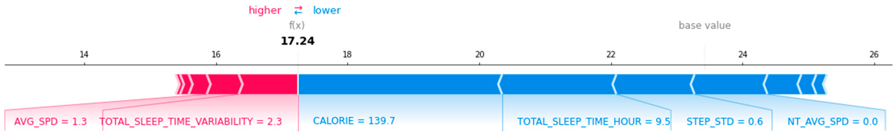
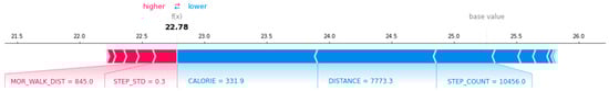
Figure A5.
Local interpretation of arbitrary data in men’s group 2 using SHAP.
Figure A5.
Local interpretation of arbitrary data in men’s group 2 using SHAP.
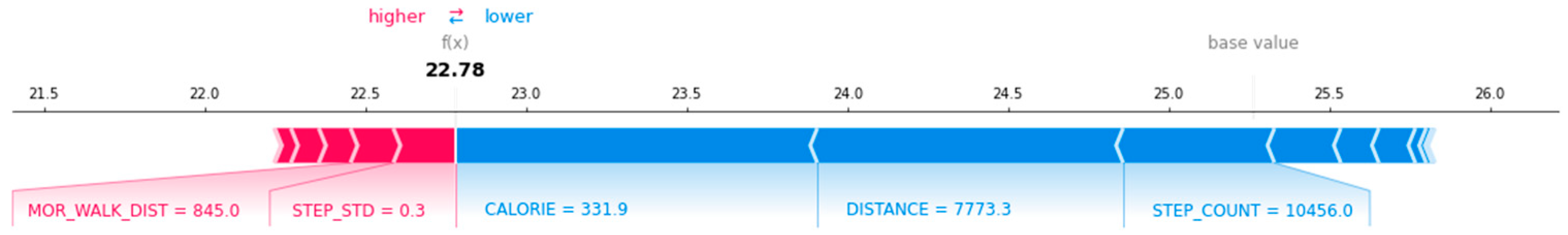
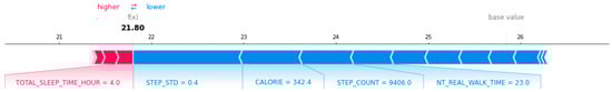
Figure A6.
Local interpretation of arbitrary data in men’s group 3 using SHAP.
Figure A6.
Local interpretation of arbitrary data in men’s group 3 using SHAP.

References
- Dodge, M.; Kitchin, R. ‘Outlines of a World Coming into Existence’: Pervasive Computing and the Ethics of Forgetting. Environ. Plann. B Plann. Des. 2007, 34, 431–445. [Google Scholar] [CrossRef]
- Kim, D.H. Effect of Walking Exercise. Korean J. Fam. Med. 2009, 30, 329–331. [Google Scholar] [CrossRef]
- Luyster, F.S.; Strollo, P.J.; Zee, P.C.; Walsh, J.K. Sleep: A Health Imperative. Sleep 2012, 35, 727–734. [Google Scholar] [CrossRef] [PubMed]
- Zheng, Y.; Manson, J.E.; Yuan, C.; Liang, M.H.; Grodstein, F.; Stampfer, M.J.; Willett, W.C.; Hu, F.B. Associations of Weight Gain from Early to Middle Adulthood with Major Health Outcomes Later in Life. JAMA 2017, 318, 255–269. [Google Scholar] [CrossRef] [PubMed]
- Wu, O.; Leng, J.H.; Yang, F.F.; Yang, H.M.; Zhang, H.; Li, Z.F.; Zhang, X.Y.; Yuan, C.D.; Li, J.J.; Pan, Q.; et al. A comparative research on obesity hypertension by the comparisons and associations between waist circumference, body mass index with systolic and diastolic blood pressure, and the clinical laboratory data between four special Chinese adult groups. Clin. Exp. Hypertens. 2018, 40, 16–21. [Google Scholar] [CrossRef] [PubMed]
- Sepp, E.; Kolk, H.; Lõivukene, K.; Mikelsaar, M. Higher blood glucose level associated with body mass index and gut microbiota in elderly people. Microb. Ecol. Health Dis. 2014, 25, 22857. [Google Scholar] [CrossRef] [PubMed] [Green Version]
- U.S. Department of Health and Human Services. Physical Activity Guidelines for Americans, 2nd ed.; U.S. Department of Health and Human Services: Washington, DC, USA, 2018.
- Public Health England. 10 min Brisk Walking Each Day in Mid-Life for Health Benefits and towards Achieving Physical Activity Recommendations; Public Health England: London, UK, 2017.
- Manson, J.; Greenland, P.; LaCroix, A.Z.; Stefanick, M.L.; Mouton, C.P.; Oberman, A.; Perri, M.G.; Sheps, D.S.; Pettinger, M.B.; Siscovick, D.S. Walking compared with vigorous exercise for the prevention of cardiovascular events in women. N. Engl. J. Med. 2002, 347, 716–725. [Google Scholar] [CrossRef] [PubMed] [Green Version]
- Jeon, C.Y.; Lokken, R.P.; Hu, F.B.; Van Dam, R.M. Physical Activity of Moderate Intensity and Risk of Type 2 Diabetes: A Systematic Review. Diabetes Care 2007, 30, 744–752. [Google Scholar] [CrossRef] [Green Version]
- Dempsey, P.C.; Larsen, R.N.; Sethi, P.; Sacre, J.W.; Straznicky, N.E.; Cohen, N.D.; Cerin, E.; Lambert, G.W.; Owen, N.; Kingwell, B.A. Benefits for Type 2 Diabetes of Interrupting Prolonged Sitting with Brief Bouts of Light Walking or Simple Resistance Activities. Diabetes Care 2016, 39, 964–972. [Google Scholar] [CrossRef] [Green Version]
- Gottlieb, D.J.; Redline, S.; Nieto, F.J.; Baldwin, C.M.; Newman, A.B.; Resnick, H.E.; Punjabi, N.M. Association of Usual Sleep Duration with Hypertension: The Sleep Heart Health Study. Sleep 2006, 29, 1009–1014. [Google Scholar] [CrossRef]
- Cappuccio, F.P.; Taggart, F.M.; Kandala, N.-B.; Currie, A.; Peile, E.; Stranges, S.; Miller, M.A. Meta-Analysis of Short Sleep Duration and Obesity in Children and Adults. Sleep 2008, 31, 619–626. [Google Scholar] [CrossRef] [PubMed] [Green Version]
- Marshall, N.S.; Glozier, N.; Grunstein, R.R. Is Sleep Duration Related to Obesity? A Critical Review of the Epidemiological Evidence. Sleep Med. Rev. 2008, 12, 289–298. [Google Scholar] [CrossRef] [PubMed]
- Patel, S.R.; Hu, F.B. Short Sleep Duration and Weight Gain: A Systematic Review. Obesity 2008, 16, 643–653. [Google Scholar] [CrossRef] [PubMed] [Green Version]
- Knutson, K.L. Sleep Duration and Cardiometabolic Risk: A Review of the Epidemiologic Evidence. Best Pract. Res. Clin. Endocrinol. Metab. 2010, 24, 731–743. [Google Scholar] [CrossRef] [Green Version]
- Gottlieb, D.J.; Punjabi, N.M.; Newman, A.B.; Resnick, H.E.; Redline, S.; Baldwin, C.M.; Nieto, F.J. Association of Sleep Time with Diabetes Mellitus and Impaired Glucose Tolerance. Arch. Intern. Med. 2005, 165, 863–867. [Google Scholar] [CrossRef] [Green Version]
- Kakizaki, M.; Inoue, K.; Kuriyama, S.; Sone, T.; Matsuda-Ohmori, K.; Nakaya, N.; Fukudo, S.; Tsuji, I. Sleep Duration and the Risk of Prostate Cancer: The Ohsaki Cohort Study. Br. J. Cancer 2008, 99, 176–178. [Google Scholar] [CrossRef] [Green Version]
- Kakizaki, M.; Kuriyama, S.; Sone, T.; Ohmori-Matsuda, K.; Hozawa, A.; Nakaya, N.; Fukudo, S.; Tsuji, I. Sleep Duration and the Risk of Breast Cancer: The Ohsaki Cohort Study. Br. J. Cancer 2008, 99, 1502–1505. [Google Scholar] [CrossRef] [Green Version]
- Thompson, C.L.; Larkin, E.K.; Patel, S.; Berger, N.A.; Redline, S.; Li, L. Short Duration of Sleep Increases Risk of Colorectal Adenoma. Cancer 2011, 117, 841–847. [Google Scholar] [CrossRef] [Green Version]
- Wu, A.H.; Wang, R.; Koh, W.-P.; Stanczyk, F.Z.; Lee, H.-P.; Yu, M.C. Sleep Duration, Melatonin and Breast Cancer among Chinese Women in Singapore. Carcinogenesis 2008, 29, 1244–1248. [Google Scholar] [CrossRef]
- Verkasalo, P.K.; Lillberg, K.; Stevens, R.G.; Hublin, C.; Partinen, M.; Koskenvuo, M.; Kaprio, J. Sleep Duration and Breast Cancer: A Prospective Cohort Study. Cancer Res. 2005, 65, 9595–9600. [Google Scholar] [CrossRef] [Green Version]
- Kolstad, H.A. Nightshift Work and Risk of Breast Cancer and Other Cancers—a Critical Review of the Epidemiologic Evidence. Scand. J. Work Environ. Health 2008, 34, 5–22. [Google Scholar] [CrossRef] [PubMed] [Green Version]
- Viswanathan, A.N.; Hankinson, S.E.; Schernhammer, E.S. Night Shift Work and the Risk of Endometrial Cancer. Cancer Res. 2007, 67, 10618–10622. [Google Scholar] [CrossRef] [PubMed] [Green Version]
- Hu, F. Obesity Epidemiology; Oxford University Press: Oxford, UK, 2008; ISBN 0-19-531291-0. [Google Scholar]
- Maclure, K.M.; Hayes, K.; Colditz, G.A.; Stampfer, M.J.; Speizer, F.E.; Willett, W.C. Weight, Diet, and the Risk of Symptomatic Gallstones in Middle-Aged Women. N. Engl. J. Med. 1989, 321, 563–569. [Google Scholar] [CrossRef] [PubMed]
- Song, M.; Hu, F.B.; Spiegelman, D.; Chan, A.T.; Wu, K.; Ogino, S.; Fuchs, C.S.; Willett, W.C.; Giovannucci, E.L. Adulthood Weight Change and Risk of Colorectal Cancer in the Nurses’ Health Study and Health Professionals Follow-up Study. Cancer Prev. Res. 2015, 8, 620–627. [Google Scholar] [CrossRef] [PubMed] [Green Version]
- Zhan, A.; Mohan, S.; Tarolli, C.; Schneider, R.B.; Adams, J.L.; Sharma, S.; Elson, M.J.; Spear, K.L.; Glidden, A.M.; Little, M.A.; et al. Using Smartphones and Machine Learning to Quantify Parkinson Disease Severity: The Mobile Parkinson Disease Score. JAMA Neurol. 2018, 75, 876–880. [Google Scholar] [CrossRef] [PubMed]
- Stankoski, S.; Jordan, M.; Gjoreski, H.; Luštrek, M. Smartwatch-Based Eating Detection: Data Selection for Machine Learning from Imbalanced Data with Imperfect Labels. Sensors 2021, 21, 1902. [Google Scholar] [CrossRef]
- Stark, G.F.; Hart, G.R.; Nartowt, B.J.; Deng, J. Predicting breast cancer risk using personal health data and machine learning models. PLoS ONE 2019, 14, e0226765. [Google Scholar] [CrossRef]
- Agarwal, A.; Saxena, A. Comparing Machine Learning Algorithms to Predict Diabetes in Women and Visualize Factors Affecting It the Most—A Step toward Better Health Care for Women; Springer: Singapore, 2020. [Google Scholar] [CrossRef]
- Zhang, Y.; Wang, S.; Hermann, A.; Joly, R.; Pathak, J. Development and validation of a machine learning algorithm for predicting the risk of postpartum depression among pregnant women. J. Affect. Disord. 2021, 279, 1–8. [Google Scholar] [CrossRef]
- Chatterjee, A.; Gerdes, M.W.; Martinez, S.G. Identification of Risk Factors Associated with Obesity and Overweight-A Machine Learning Overview. Sensors 2020, 20, 2734. [Google Scholar] [CrossRef]
- Pinto, K.A.; Abdullah, N.L.; Keikhosrokiani, P. Diet & Exercise Classification using Machine Learning to Predict Obese Patient’s Weight Loss. In Proceedings of the International Congress of Advanced Technology and Engineering (ICOTEN), Taiz, Yemen, 4–5 July 2021; pp. 1–5. [Google Scholar] [CrossRef]
- Eoghan, K. BorutaShap: A Wrapper Feature Selection Method Which Combines the Boruta Feature Selection Algorithm with Shapley Values. (1.1); Zenodo: Geneva, Switzerland, 2020. [Google Scholar] [CrossRef]
- Kursa, M.B.; Rudnicki, W.R. Feature Selection With the Boruta Package. J. Stat. Soft. 2010, 36, 1–13. [Google Scholar] [CrossRef] [Green Version]
- Bhalaji, N.; Kumar, K.S.; Selvaraj, C. Empirical study of feature selection methods over classification algorithms. Int. J. Intell. Syst. Technol. Appl. 2018, 17, 98–108. [Google Scholar] [CrossRef]
- Strobl, C.; Boulesteix, A.-L.; Zeileis, A.; Hothorn, T. Bias in random forest variable importance measures: Illustrations, sources and a solution. BMC Bioinform. 2007, 8, 25. [Google Scholar] [CrossRef] [PubMed] [Green Version]
- Joharestani, M.Z.; Cao, C.; Ni, X.; Bashir, B.; Talebiesfandarani, S. PM2.5 Prediction Based on Random Forest, XGBoost, and Deep Learning Using Multisource Remote Sensing Data. Atmosphere 2019, 10, 373. [Google Scholar] [CrossRef] [Green Version]
- Voskresenskiy, A.; Bukhanov, N.; Filippova, Z.; Brandao, R.; Segura, V.; Brazil, E.V. Feature Selection for Reservoir Analogues Similarity Ranking As Model-Based Causal Inference. In Proceedings of the Conference Proceedings, ECMOR XVII, Online, 14–17 September 2020; Volume 2020, pp. 1–9. [Google Scholar] [CrossRef]
- National Health Insurance Service, Average Height Distribution by Province, Age, and Gender: General. Available online: https://kosis.kr/statHtml/statHtml.do?orgId=350&tblId=DT_35007_N130 (accessed on 23 September 2021).
- Lee, S.-J.; Kim, Y.-J.; Kim, T.-W.; Ahn, S.-J. New Evaluation Chart of Stature and Weight for Koreans. Korean J. Orthod. 2006, 36, 153–160. [Google Scholar]
- Hollis, J.L.; Williams, L.T.; Young, M.D.; Pollard, K.T.; Collins, C.E.; Morgan, P.J. Compliance to step count and vegetable serve recommendations mediates weight gain prevention in mid-age, premenopausal women. Findings of the 40-Something RCT. Appetite 2014, 83, 33–41. [Google Scholar] [CrossRef] [Green Version]
- Browning, R.C.; Kram, R. Effects of obesity on the biomechanics of walking at different speeds. Med. Sci. Sports Exerc. 2007, 39, 1632–1641. [Google Scholar] [CrossRef]
- Amorim, P.; Moura, B.P.D.; Marins, J. Self selected walking speed in overweight adults: Is this intensity enough to promote health benefits? Apunt. Sports Med. 2010, 45, 11–15. [Google Scholar]
- Baron, K.G.; Reid, K.J.; Kern, A.S.; Zee, P.C. Role of sleep timing in caloric intake and BMI. Obesity 2011, 19, 1374–1381. [Google Scholar] [CrossRef] [PubMed]
- Meyer, K.A.; Wall, M.M.; Larson, N.I.; Laska, M.N.; Neumark-Sztainer, D. Sleep duration and BMI in a sample of young adults. Obesity 2012, 20, 1279–1287. [Google Scholar] [CrossRef]
- Marouli, E.; Del Greco, M.F.; Astley, C.M.; Yang, J.; Ahmad, S.; Berndt, S.I.; Caulfield, M.J.; Evangelou, E.; McKnight, B.; Medina-Gomez, C.; et al. Mendelian randomisation analyses find pulmonary factors mediate the effect of height on coronary artery disease. Commun. Biol. 2019, 2, 119. [Google Scholar] [CrossRef]
- Nelson, C.P.; Hamby, S.E.; Saleheen, D.; Hopewell, J.C.; Zeng, L.; Assimes, T.L.; Kanoni, S.; Willenborg, C.; Burgess, S.; Amouyel, P.; et al. CARDIoGRAM + C4D Consortium. Genetically determined height and coronary artery disease. N. Engl. J. Med. 2015, 372, 1608–1618. [Google Scholar] [CrossRef] [PubMed] [Green Version]
- Cho, M.; Kim, J.Y. Changes in physical fitness and body composition according to the physical activities of Korean adolescents. J. Exerc. Rehabil. 2017, 13, 568–572. [Google Scholar] [CrossRef] [PubMed] [Green Version]
- Gorostegi-Anduaga, I.; Corres, P.; Aguirre-Betolaza, A.M.; Pérez-Asenjo, J.; Aispuru, G.R.; Fryer, S.M.; Maldonado-Martín, S. Effects of different aerobic exercise programmes with nutritional intervention in sedentary adults with overweight/obesity and hypertension: EXERDIET-HTA study. Eur. J. Prev. Cardiol. 2018, 25, 343–353. [Google Scholar] [CrossRef] [PubMed]
- Rowlands, A.V.; Ingledew, D.K.; Eston, R.G. The effect of type of physical activity measure on the relationship between body fatness and habitual physical activity in children: A meta-analysis. Ann. Hum. Biol. 2000, 27, 479–497. [Google Scholar]


Publisher’s Note: MDPI stays neutral with regard to jurisdictional claims in published maps and institutional affiliations. |
© 2022 by the authors. Licensee MDPI, Basel, Switzerland. This article is an open access article distributed under the terms and conditions of the Creative Commons Attribution (CC BY) license (https://creativecommons.org/licenses/by/4.0/).