Abstract
The sorting of biological cells or particles immersed in a fluid is a frequent goal in the domain of microfluidics. One approach for such sorting is in using the inertial effects that are present in curved channels. In this study, we propose a new approach of inertial focusing of cells in microfluidic devices. The investigated channels had the form of a helical channel with a circular cross-section, and the cells were spherical. We identified the key parameters that influence the cell sorting results through multiple computational simulations using a modelling tool PyOIF within the package ESPResSo. We found that spherical cells could be sorted with respect to their size in helical channels since their stabilised positions are located in different parts of the channel cross section. The location of the stabilised position is a function of the fluid parameters, the geometrical parameters of the helical device, and the size of the immersed cells.
1. Introduction
The precise control of the cell motion is essential in microfluidics. One method to do this is to exploit inertial effects. Inertial microfluidics are utilized to sort different types of cells, as a function of their size and their physical properties, such as deformability and shape. There are different channel shapes that are suitable for cell separation or focusing—for example, a 2D spiral channel [1,2], a laminar vortex technology [3], or zig-zag curved channels [4]. A general overview of the available techniques and their physical background can be found in [5], and a description of inertial techniques with respect to clinical use can be found in [6].
In this study, we consider almost rigid spherical cells in a helical channel. Inertial sorting in helical channels was also used in [7] where the authors considered a helical channel with a trapezoid cross-section. Their aim was to detect E. coli bacteria in a real food matrix. In [8], a commercially available capillary tube with a squared cross-section was used to focus micro-beads of different sizes. Other aspects of particle focusing within a helical micro-channel were studied in [9,10].
The advantage of a helical channel is that the particle separation efficiency can be adjusted by modifying the geometry of the channel—by adjusting the 3D coiling radius of a single device rather than using multiple devices with a different designs. This idea was exploited by using flexible pipes used to create the helical channel [8,9]. The basic principle of inertial sorting is the balance of the Dean force and the lift force acting on a particle. The particle finds its stabilized position within the cross-section in a place where the magnitudes of these two forces are almost equal and the directions are the opposite.
This principle is often difficult to achieve since both the Dean force and the lift force partially depend on the same quantities with different orders of magnitude. It is delicate to find a balance so that one force does not dominate the other [11]. In this study, we considered a different approach. We considered Dean-force-dominated flows where the stabilized position is not the result of an equilibrium between the Dean and the lift force.
The Dean force is dominant over the lift force in the examined geometries. Therefore, the stabilized position is mainly defined by a place where the Dean force vanishes, which is close to the centre of the Dean vortices. In this paper, we show that smaller cells tend to stabilise in the lower part of the channel and larger cells in the upper part. This finding has a practical implication: By suitable design of the channel output with two branches, one can collect larger cells and smaller cells in different outlets. In our work, we show that this is possible, and we suggest concrete dimensions of the helix to achieve this behaviour.
In the following sections, we first present the theoretical background for our approach in sorting cells in a helical channel. Then, we present a setup for the numerical simulation where the sorting of microbeads was observed. After that, we perform a sensibility analysis—we examined the sensibility of the results to the modification of specific physical parameters linked to fluid flowing through the channel, or parameters linked to channel geometry. In the end, we present also a stability analysis—a sensibility analysis of the results with modification of the numerical parameters.
2. Theoretical Background
The forces acting on a spherical particle in a curvilinear flow are complex. There are two types of forces: lateral-flow-induced forces called lift forces and transversal, or secondary-flow-induced forces, called Dean forces. We review the basic mechanisms for these forces [5].
2.1. Lift Force
The lift force is composed from the wall-induced force and shear-gradient-induced force. The combination of these two forces lies in a Segré–Silberberg effect in straight channels [12]. The stabilised positions of particles in straight channels depend on the cross-section of the channel, the physical parameters of the particles, and the physical parameters of the fluid [5,13].
When a cell is sufficiently close to a wall, the wall-induced force arises from different pressures in the fluid that flow around the cell. In the constriction between the wall and the particle, the pressure will not be changed. On the other side of the particle, the streamlines will become denser, and thus the fluid velocity will be larger; therefore, the pressure will decrease. This will cause a force directed away from the walls of the channel. The formula that describes the magnitude of the wall-induced force is
where is a lift coefficient dependent on the particle position and on the Reynolds number [14], is the fluid density, is the maximal fluid velocity, a is the particle diameter, and is the hydraulic diameter of the channel.
The shear-gradient-induced force arises also from a different velocity profile around the cell; however, this one takes its origins in the parabolic velocity profile. The magnitudes of fluid velocities on the two sides of the cell are different. The force that is acting on cell due to this difference pushes the cell closer to the wall. The formula that describes the magnitude of the shear-gradient-induced force is
where is a shear coefficient dependent on particle position and on Reynolds number [14].
The final lift force is sum of the wall-induced force and shear-gradient-induced force. The formula for the total lift force is not the same across the literature. In [14], where a squared cross-section was examined, the final lift force is either the wall-induced force or the shear-induced force, as a function of the particle position. For particles closer to the centre of the cross-section, the shear-induced force is dominant, whereas for particles that are closer to the channel walls, the wall-induced force is dominant.
Several authors agree on the following formula for the lift force, e.g., [7],
where is the lift coefficient as a function of the particle position within the channel cross-section, considered to be 0.5 for simplification. This formula is taken from a study where a spherical particle in a straight channel with plane Poiseuille flow at large channel Reynolds number was examined [15].
In our study, the geometry and the range of Reynolds numbers is more similar to [14]; therefore, we consider the same expressions for the lift force as used in this study.
The final formula, however, is tricky: As we have seen, even in straight channels, it is impossible to write down an explicit dependence of the forces depending on the flow parameters. Even the well-accepted formula (3) appearing in [15] contains a lift coefficient depending on the position of the particle in a channel and the channel Reynolds number. This dependence is not listed in the original works. Moreover, in [14], the authors showed that the term changes to in near-centre regions and to in near-wall regions without further specifying what “near” means. Not to mention that the might change as well. Therefore, the actual simulations of scenarios with curvilinear channels are crucial for the correct determination of stable positions in channels.
2.2. Dean Force
The Dean force is linked to Dean vortices in curved geometries. The origin of this secondary flow is a parabolic fluid flow within the cross-section. The fastest fluid, which is approximately in the centre of the cross-section, undergoes the highest centrifugal force. Therefore, it is pushed outward away from the centre of curvature. The rest of the fluid within the cross-section conforms to the movement of this fastest fluid, and this results in a pair of symmetric Dean vortices. The intensity of the secondary flow is dependent on the intensity of the primary flow but not linearly [1,16].
The Dean force acting on a particle in a flow can be evaluated as follows
where is the dynamic viscosity, a is the particle diameter, and is the local velocity of the Dean flow—the transversal velocity within the Dean vortex at the particle location.
To assess the value of the Dean force acting on a particle, we need to know the inertial velocity of the fluid in the particle position, the . However, this velocity is not clearly defined across the literature.
In [17], the average Dean velocity is found to be
where is the Dean number, which is a dimensionless number that characterizes transversal effects and can be calculated as
with being the Reynolds number and the curvature radius of the channel.
Using (5) for the average Dean velocity, the formula for the average Dean force acting on a particle would be
However, (5) and (7) should be used with caution. Both formulae were determined from an experiment with fixed geometry, where the curvature radius was significantly larger than in our study.
Another formula used in the literature [4,11] gives us an equation to calculate the maximal Dean velocity as
and then the maximal Dean force becomes
However, the authors in these works do not specify any parameter or a constant that would define more precisely the value of the , additionally to a statement that it is proportional to a combination of the simulation parameters as we can see in (8). We can expect that this parameter would be not a simple constant but a variable depending on a position of the particle, or on the Reynolds or the Dean number.
For a fixed simulation setup, the Dean drag force would be different across the cross-section of the channel, as the velocity in the Dean vortices is not the same within the cross-section. The previous formulae proposed only rough estimates of the values of the forces acting on a particle. We can see that the analytical calculation of the lift and Dean forces are not clear, and thus numerical simulations can help to better understand the trajectories of particles immersed in curved channels.
2.3. (Non-) Equilibrium of Dean and Lift Forces in Helical Channels
In Appendix A, we analyse the magnitudes of Dean forces and lift forces in our settings. We concluded that the lift force over the Dean force ratio is significantly less than one.
In our work, we therefore did not set the geometry of the microfluidic device in order to equilibrate the Dean and the lift force in the way described in previous articles. The Dean drag force depends on the velocity of the secondary flow. Therefore, it is variable across the cross-section perpendicular to the main flow. The magnitude of the Dean force is significantly larger near the circumference of the Dean vortices than near the centres of the vortices where it vanishes.
Therefore, the equilibrium between the lift and the Dean force is obtained in a zone where the Dean force achieves a fraction of its maximal magnitude, which is close to the centres of vortices. In the following sections, we consider a certain set up of numerical experiment as a baseline, and we modify several experimental parameters one by one. We examine the change of lift force over the Dean force ratio, caused by the variation of these experimental parameters.
The ratio of wall-induced lift force over the maximal Dean force is computed from (1) and (9)
while the ratio of shear-induced lift force over the maximal Dean force is computed from (2) and (9)
where and are coefficients depending on the coefficients and and the parameters that appear in the formula for the Dean force (6).
In an ideal case, the two ratios would help us to evaluate the impact of modification of the experimental parameters on the focusing ability of the microfluidic device. However, we see that this will not always be the case. The parameters and are dependent on several other variables, such as the particle position, or Dean number—hence, the fluid velocity, fluid viscosity, channel geometry, etc.
2.4. Description of the Numerical Model
The liquid in our model is calculated using the lattice–Boltzmann (LB) method [18]. This method uses fictitious particles that propagate and collide over a fixed three-dimensional discrete lattice. For most simulations, we used a grid of 1 m. The particle density function is defined for each lattice point , discrete velocity vector and time t. We use the D3Q19 version of the LBM (three dimensions with 19 discrete directions along the edges and diagonals of the lattice). The governing equations are
where is the time step, and denotes the collision operator that accounts for the difference between pre- and post-collision states and satisfies the constraints of mass and momentum conservation. This collision operator also includes —the external forces exerted on the fluid that come from expression (14).
The cells are taken into account as an immersed objects with fully 3D discretization using tetrahedrons that cover the whole inner space inside the sphere. At the edges of the small tetrahedrons, fairly rigid springs are set so that the object undergoes almost no deformation during the flow. The springs are modelled using stretching forces that tend to preserve a relaxed length of the edge between vertices . The stretching force acting on vertex A is defined as
with the opposite force for vertex B. With high enough, one obtains rigid spheres as cells. Detailed descriptions of the underlying models are available in [19,20,21]. The validation and verification of the computational models has been provided in [22,23,24]. For all simulations, we used tetrahedral meshes with edges of sizes approximately 0.4 m.
Both fluid and cell discretizations are coupled by dissipative force coupling enforcing the no-slip condition such that the force exerted by the fluid on one mesh point is proportional to the difference of the velocity of the mesh point and the fluid velocity at the same position,
where is a frictional coupling parameter calibrated in [25].
Elastic forces together with fluid force F compose a total force acting on cell mesh points that causes motion according to Newton’s equation:
where m is the mass of the mesh points.
The calculations of the fluid are performed on a GPU [26]. The calculation of immersed cells is performed on a CPU. Due to low number of cells, this does not cause performance issues.
3. Setup of the Numerical Simulation
The geometry of the baseline reference solution is depicted in Figure 1. We have chosen this geometry because we observed different type of trajectories for two different cells in this helical channel, and consequently different stabilised positions. One such trajectory is indicated in the figure on the left as a blue helical line. Its projection onto the cross-section (cross-section = a plane that is perpendicular to the local axis of the helix) is indicated as a dense blue spiral on right of the figure.
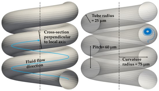
Figure 1.
The geometry of the helix used in the reference simulation. The blue curve at the right side stands for the projection of a cell trajectory to a cross-section that is perpendicular to the local helix axis.
The simulation box contained only one loop of the helix, in order to reduce the computational cost. The cyclic boundary conditions ensure the continuity of the simulation on both ends of the channel, and thus the helical channel is modelled as a channel with infinite length.
Both cells used in simulations were spherical and almost rigid, they differed only by their size. We chose only two different cell diameters of 4 and 7.82 m as two use-cases. The actual values were motivated by the size of red blood cells and smaller cells. For sorting larger cells, the dimensions of the helix could be scaled up with similar qualitative results. The discretization of a cell’s inner volume was used in order to ensure their rigidity. To maintain a similar density of discretization points with respect to the discretization of the fluid, the larger cell was discretized with more nodes. The sizes of cells and their discretization are listed in Table 1. The spatial discretization of the fluid was m, and all the simulations were run with a simulation timestep of s.

Table 1.
The size and discretization of the cells present in the set of simulations.
Starting from this reference simulation, we modified several parameters linked to the fluid as well as parameters linked to the geometry of the helical channel. The examined parameters and their values are listed in Table 2. As the maximum fluid velocity, we took the maximal velocity magnitude found in the velocity field. The maximum velocity was oriented parallel with the local axis of the helix curvature. Throughout all the simulations, we used a fixed fluid density of water.
Table 2.
List of the examined parameters in our simulations.
The “Reference” line in the table stands for the reference simulation. The results of all the other simulations were compared with the reference simulation to establish the stability analysis. In each simulation, we modified only one parameter among the considered parameters listed in Table 2. This means that each field in rows Mod 1–Mod 4 corresponds to one simulation setting, in which we kept all the parameters from the reference simulation, except the one parameter, which was modified as it is specified in the field’s value. The majority of these sensibility studies were run twice—once with the smaller cell and a second time with the larger cell. Only in the case of the pitch and the tube radius, we chose different parameter values for different cell sizes.
The range of Reynolds numbers used in simulations was from 2.5 to 10, and the reference simulation had a Reynolds number of 5. The Dean numbers ranged from 1 to 6, and the reference simulation had Dean number of 3.
4. Results—Effects of the Simulation Parameters on the Cell’s Trajectory
In this section, we present our observed trajectories of cells. All the trajectories are presented as their projection on the circular cross-section, which is perpendicular to the local axis of the helix; see Figure 1.
4.1. Streamlines of the Fluid Flow
In Figure 2, we can see streamlines of the inertial flow inside the helix for the reference set of parameters. The streamlines were observed from a simulation without cells using stream tracers that do not influence the flow. We can observe the fluid streamlines on one hand, and the trajectory of the stream-tracers on the other hand. While the streamlines are rather symmetric, the trajectories of the isolated point tracers show an asymmetric tendency. We expected to obtain similar images, the inertia-less particle tracers should follow a trajectory that is defined by fluid streamlines. The difference in the observed Dean vortices—a rather symmetric pair of vortices on one hand, and a considerably inequal pair of vortices on the other hand—is rather perplexing at the moment.
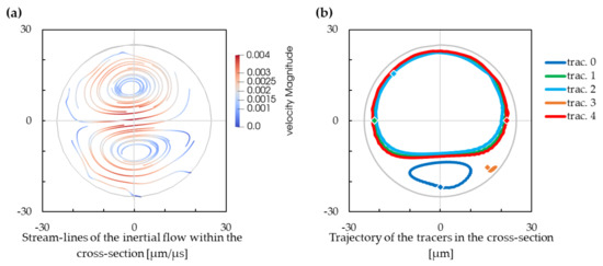
Figure 2.
(a) Streamlines of an inertial flow. Negative values on the x-axis are for the inner wall of the cross-section, and positive values are for the outer wall of the cross-section. Projection of the streamlines to a plane that is perpendicular to the local axis. (b) Projection of the stream-tracer trajectory to a plane that is perpendicular to the local axis. The initial positions of the tracers are marked with diamonds.
4.2. Reference Solution
The trajectory of solid cells is influenced by their size and, if they are small enough, by their initial position. In Figure 3, the cell with a radius of m has only one stabilised position, which is eventually reached from any starting point within the cross-section. The cell with a radius of m has, however, two different stabilised positions. The upper one is reached when the starting position of the cell is approximately in the upper 3/4 of the channel, while the lower one is reached from the lower quarter of the channel cross-section.
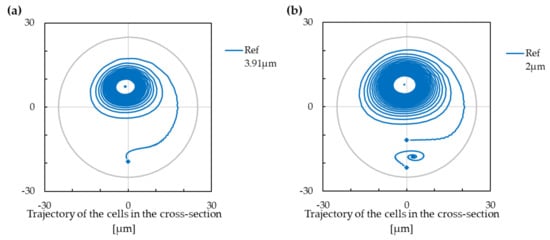
Figure 3.
The trajectory and stabilised positions for the reference case. The starting positions of cells are marked with diamonds. Negative values on the x-axis are for the inner wall of the cross-section, and positive values are for the outer wall of the cross-section. (a) The cell with a radius of m has only one stabilised position. (b) The cell with a radius of m has two different stabilised positions.
In Figure 4, there is a dashed separation line that divides the cross-section into two parts. Smaller cells starting from the lower part converge to the lower stabilized position, whereas those starting from the upper part converge to the upper stabilized position. This line is defined by the trajectories of the smaller cells, and it is at around m below the centre of the cross-section for this case.
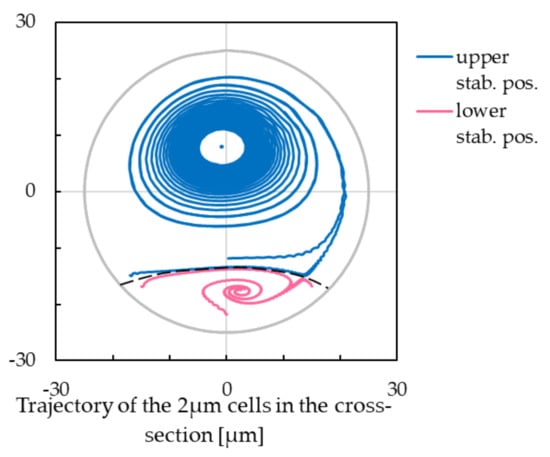
Figure 4.
The separation line between the upper and lower stabilised position for cells with m radius. Cells starting their trajectory below the separation line will reach the lower stabilised position, while the cells starting above this line will reach the upper stabilised position.
Separation of cells with two different sizes can be achieved by a proper installation of inlets and outlets to and from the helical structure. If the inlet of a cell mixture is located below the dashed line, smaller cells converge to lower stabilized position and large cells to the upper one resulting in their separation. Finally, two outlets can be installed so that one collects larger cells and one the smaller ones.
We can see in this picture that the the stabilized position is not reached directly but rather after many concentric turns following a spiral path. Therefore, in the next section, we do not show the exact stabilised position. We show only the onset of the trajectory, from which it will be clear whether there are one or two different stabilised positions. For the clarity of the images, the trajectories of the reference solution are presented only by their onset.
The position of the dashed separation line can also help us to define minimal length of the helical tube for sorting the cells. We need to ensure the helical tube is long enough, and thus the large cells will traverse through the separation line from any starting position in the lower part of the cross-section. The smaller cells will all remain below the separation line, as they will become stabilised in the lower part of the channel.
The larger cell traverses the separation line relatively fast in this case. It crosses the line once, and then it stays in the upper part during its elliptical converging trajectory. This might not always be the case. For certain combination of the experimental parameters, the larger cell may re-descend to the lower part of the cross-section and then go back up again several times during its elliptical motion. However, in our case, the larger cell needs to travel a total distance of m in the direction of the global helix axis, which is approximately six loops of the helix with the pitch of m, until the cell remains above the separation line.
The ratio of wall-induced lift force over the shear-induced lift force is proportional to . The wall-induced lift force of larger cell is thus larger, which explains why the smaller cells can have one more focusing position that is relatively close to a wall: The wall-induced lift force is too large in the case of a larger cell, it pushes out the larger cell from the regions close to the walls.
Therefore, the decrease in the cell’s diameter may lead to increasing the number of stabilised positions from one to two, or to increasing the cross-section area below the dashed line that leads to the lower stabilised position.
4.3. Dimensionless Reynolds Number and Dean Number
Instead of varying the individual parameters of the simulation to study the resulting effect on the cell’s trajectories, one can modify the dimensionless numbers that characterize the simulation setup. We tested whether the constant gives us the same results even with different physical parameters. We found that varying gives the same results (or at least very similar) as varying the fluid viscosity while keeping the same . Since the fluid velocity enters the Reynolds number in the numerator, and the kinematic viscositye enters in the denominator, doubling the velocity gives the same effect on as halving the viscosity and vice versa. Comparing the results for this doublet of simulations gave almost identical trajectories of the cells; see Figure 5. Therefore, in further analyses, we restricted ourselves to the modification of only.
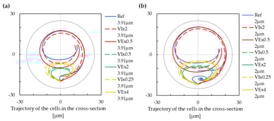
Figure 5.
The trajectory of cells with modification of the Reynolds number. Two lines (solid and dashed) with the same colour depict the trajectory with the unchanged. Negative values on the x-axis are for the inner wall of the cross-section, and positive values are for the outer wall of the cross-section. (a) The cell with a radius of m. (b) The cell with a radius of m.
On the other hand, we tested whether the same was applicable to the Dean number. We modified the geometry from the reference simulation in two ways: First, we doubled the curvature radius , and second we multiplied by 0.8, which, in the third power, gives again approximately 1/2 in the fraction under the root in expression (6). In Figure 6, we clearly see that the red and green lines are different, leading to different stabilized positions. This can be explained by the fact that the inertial effects resulting from curved channels are influenced not only by the curvature radius and tube radius but also by the pitch of the helix. In this view, a helix is quite a unique geometry.
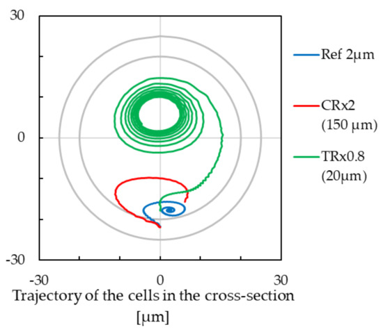
Figure 6.
The trajectory of cells with modification of the curvature radius (CR) or tube radius (TR) of the channel, for the cell with a radius of m. Negative values on the x-axis are for the inner wall of the cross-section, and positive values are for the outer wall of the cross-section. The outer circle stands for the circumference of the the m cross-section, and the inner circle is for the circumference of the m cross-section.
4.4. Modification of the Fluid Parameters: Maximum Fluid Velocity
The trajectories of the cells can be seen in Figure 7. The reduction of the velocity either reduced the number of stabilized positions from two to one (in the case of the smaller cell), or it decreased the share of the cross-section area related to the lower stabilised position (in the case of the larger cell). The increase in the flow velocity, on the other hand, added the second stabilized position (in the case of the smaller cell), or it increased the area share of the lower stabilised position (in the case of the larger cell).
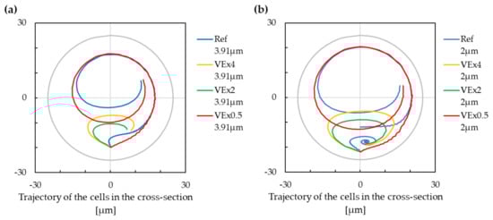
Figure 7.
The trajectory of cells with modification of the fluid velocity. Negative values on the x-axis are for the inner wall of the cross-section, and positive values are for the outer wall of the cross-section. (a) The cell with a radius of m. (b) The cell with a radius of m.
From (10) and (11), we can see that the lift force over the Dean force ratio does not change with modification of the maximum fluid velocity. However, as in the previous paragraph, this can be explained by the influence of the pith that is not included in the expression for the Dean number.
The increasing of the fluid velocity thus has as a consequence in that it enables differentiation between the cells according to their size.
4.5. Modification of the Helical Microchannel Geometry: Helix Pitch
In the following sections, we discuss the trajectory modification induced by changes in the channel geometry. The first examined parameter is the helix pitch, which is the distance between centres of two adjacent helical loops. The reference pitch was already relatively small and difficult to decrease: with a radius of cross-section m and pitch m, there is only m left of free space between the edges of two adjacent loops. Therefore, we tested only values of the helix pitch that were larger than the reference one.
There was an evident impact of helical pitch in both cases—for the larger and for the smaller cell; Figure 8. In the case of the larger cell, the increase in the helix pitch changes the final location of the stabilised position, while with a smaller pitch of m, the stabilised position is in approximately in the upper 2/3 of the cross-section. With the pitch of m, it is closer to the centre of the cross-section. We can see a similar shift in the case of the smaller cell. The pitch of m leads to two different stabilised positions, a lower one and an upper one. With an increase in the pitch, the lower stabilised position (if it exists) vanishes, and the upper stabilised position becomes closer to the centre of the cross-section.
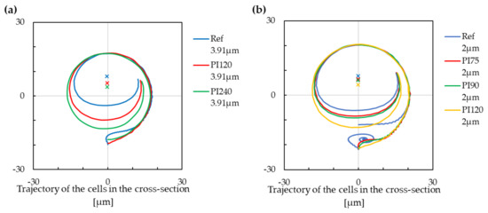
Figure 8.
The trajectory of cells with modification of the helix pitch. Cross markers denote the extrapolated stabilized positions. Negative values on the x-axis are for the inner wall of the cross-section, and positive values are for the outer wall of the cross-section. (a) The cell with a radius of m. (b) The cell with a radius of m.
Reaching the stabilised position takes a longer time in channels with higher values of the pitch. This is reasonable if we consider a helical channel as an intermediate channel between two extremes—a torus and a perfectly straight channel. In a torus, the particles would follow the flow induced by Dean vortices; therefore, they will flow in circular-like trajectories (as we already saw in other helices that are more similar to a torus in their pitch). In a perfectly straight channel, the particles would slowly change their position within the cross-section and focus in a specified distance between the centre of the tube and its circumference. Eventually, they would create a set of focusing positions as a circumscribed circle (Segré–Silberberg effect). In a helix, the particles would flow in circular-like trajectories, and their initial position as a distance from the centre of the cross-section would change only slowly.
We notice that the decreasing of the pitch may lead to adding another stabilised position (in the case that there was only one), or to increasing of cross-section area linked to the lower stabilised position (in the case of two stabilised positions). From this, we can draw similar conclusion as with increasing the fluid velocity: The decreasing the pitch enables differentiation between the cells according to their size.
4.6. Modification of the Helical Microchannel Geometry: Curvature Radius
The modification of the helix curvature radius has an opposite impact to the cell trajectories compared to the modification of the helix pitch. In Figure 9, we can see that the higher values of the curvature radius lead to a new stabilised position in the lower part of the cross section for the larger cell. The lower stabilised position of the smaller cell stays in the lower part of the channel, and the convergence area is larger. With the decreasing curvature radius, we can make a similar observation as for the increasing helix pitch—the stabilized position (if it exists) vanishes, and the stabilised position in upper part of the cross-section moves towards the centre of the cross-section.
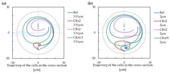
Figure 9.
The trajectory of cells with modification of the curvature radius. Cross markers denote the extrapolated stabilized positions. Negative values on the x-axis are for the inner wall of the cross-section, and positive values are for the outer wall of the cross-section. (a) The cell with a radius of m. (b) The cell with a radius of m.
The curvature radius and the helix pitch are two parameters that altogether influence the trajectory and the stabilised position of the cells in very similar way as we already saw in the case of fluid velocity and fluid viscosity.
With the increasing value of , the local geometry of the helix becomes more similar to a torus geometry—the pitch value is less important in comparison with . Therefore, the trajectory of the cells is more similar to a trajectory observable in torus, copying two Dean vortices. This effect is noticeable also in our results. With larger curvature radius, we can see that the lower part of the circular cross-section enclose a new stabilised position in case of the larger cell. In the case of the smaller cell, the existing separation line between two stabilised positions moves closer to the centre of the cross-section.
From (10) and (11), the lift force over the Dean force ratio changes with ∼. Increasing the curvature radius makes the Dean force less important comparied to the total lift force. The increasing of curvature radius yields to adding another stabilised position (in the case that there was only one), or to increasing of cross-section area linked to the lower stabilised position (in the case of two stabilised positions). From this, we can again draw similar conclusion as with increasing the fluid velocity or decreasing the pitch: The increase of the curvature radius enables differentiation between the cells according to their size.
Curvature Radius Influences the Transversal Speed of Cells
Decreasing increases the moment of inertia, and this affects the transversal speed of cells. To illustrate this observation, we simulated a fixed time of 10 ms for different . For a curvature radius of 150 m, the cell passed approximately 17 m within the perpendicular cross-section during 10 ms of the simulation. With a curvature radius of 75 m, the cell passed approximately 113 m during the same time, and for a curvature radius of 37 m, the cell passed approximately 47 m.
For smaller cell, it passed 101 m in the case of the smallest radius curvature, 35 m in the case of the reference radius curvature, and 13 m in the case of the largest radius curvature, all within 10 ms of simulation. The observed trajectories are depicted in Figure 10.
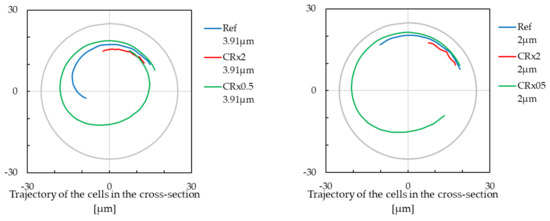
Figure 10.
The length of the cell trajectory with modification of the curvature radius over 10,000 s of simulation. Negative values on the x-axis are for the inner wall of the cross-section, and positive values are for the outer wall of the cross-section. Left, the cell with a radius of m. Right, the cell with a radius of m.
4.7. Modification of the Helical Microchannel Geometry: Tube Radius
The trajectories of the smaller cell in a channel with a modified tube radius are shown in Figure 11. The tube radius was difficult to increase from the same reason as the modification of the helix pitch. The space between two adjacent loops was already quite small in the reference case; therefore, we did not had much space to increase the tube parameter. From this reason, we tested only smaller values of the tube radius in comparison with the reference case. The tests were made only for the smaller cell. We can observe that the lower stabilised position vanished for both examined values of tube radius, and the cell converged to an upper stabilised position.
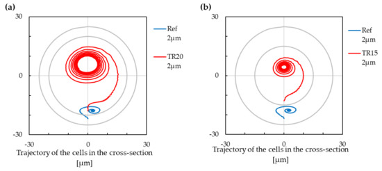
Figure 11.
The trajectory of cells with modification of the tube radius. Negative values on the x-axis are for the inner wall of the cross-section, and positive values are for the outer wall of the cross-section. (a) The cell with a radius of m. The outer circle stands for circumference of m cross-section, the inner circle for circumference of m cross-section. (b) The cell with a radius of m. The outer circle stands for circumference of m cross-section, the inner circle for circumference of m cross-section.
With using (10) and (11), the lift force over the Dean force ratio change with ∼ for the shear-gradient-induced lift force and with ∼ for the wall-induced lift force. With increasing the tube radius, the total lift force becomes less important in comparison with Dean force. The trajectory of the cell is, thus, driven mainly by the Dean force for channels with a large tube radius. This is also what we can observe in our case—the cells are dragged by Dean vortices in the case of the larger tube, and there are two stabilised positions defined by positions of the Dean vortices.
The increasing of tube radius yields to adding another stabilised position (in the case that there was only one), or to increasing the cross-section area linked to the lower stabilised position (in the case of two stabilised positions). Therefore, the increasing of the tube radius enables differentiation between the cells according to their size.
5. Numerical Convergence
To justify the choice of time and space discretizations, we performed tests of numerical convergence by varying two numerical parameters—the timestep and spatial discretization lb-grid. The tested combinations of parameter values are presented in Table 3. The other simulation parameters were the same as in the reference case, and the simulations were run only with the smaller cell.
Table 3.
The tested numerical parameters—time and space discretization. With x we marked performed simulations, while - denote omitted simulations.
In Figure 12 and Figure 13, we can see the effect of those parameters on the cell trajectory. The spatial discretization should be put into context also with discretization of the immersed cell.
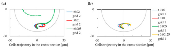
Figure 12.
The trajectory of cells for variable values of timestep. Negative values on the x-axis are for the inner wall of the cross-section, and positive values are for the outer wall of the cross-section. (a) grid value m. (b) grid value m.
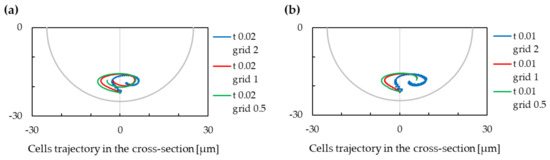
Figure 13.
The trajectory of cells for variable values of spatial grid. Negative values on the x-axis are for the inner wall of the cross-section, and positive values are for the outer wall of the cross-section. (a) Timestep value s. (b) Timestep value s.
We can observe that the setting of these numerical parameters can significantly change the results of the simulation—in one of observed cases, with timestep s and grid m, the cell did not find a stabilised position in the lower part of the channel cross section. However, in most of cases, the cell is focused in the lower part.
In Figure 13, we can observe an impact of the grid modification to the cell trajectory. We can notice that the difference between simulations with a grid of m and m are not significant, while the difference between simulations with grid of m and m is more important. We can conclude that simulations with m grid are hence not sufficiently discretized as refinement of the mesh changes the results significantly. This conclusion can be made also from observation of Figure 12, where we can see that modification of the timestep does not significantly influence the results with a grid of m; however, the results are less stable with a grid of m.
From this analysis of numerical convergence, we concluded that the suitable values for parameters in Section 4 are m for the timestep and 1 for the lb-grid.
6. Discussion
The obtained results show us a possibility of sorting cells according to their size in helical channels. The parameters of the channel can be adjusted in order to obtain stabilized positions of the cells situated in a convenient vertical position within the channel cross-section.
The cell sorting can be obtained by using proper inlets and outlets of the channel, as proposed in Figure 14. The inlets here are two separate tubes, one of them injected a cell-free buffer liquid and leading to the upper part of the circular cross-section above the dashed horizontal line (see Figure 4) that separates the upper and lower stabilized position for the smaller cells. The second inlet tube contains a suspension of cells that should be sorted. This inlet tube leads into the lower part of the helical cross-section below the dashed line. This results in stabilizing the smaller cells in the lower part of the channel. The larger cells can escape from this lower part and become stabilized in the upper part.
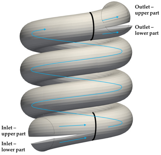
Figure 14.
The proposed shape for inlets and outlets for the helical channel.
The outlet is composed of two tubes as well. The tube that comes from the upper part of the cross section collects the larger cells, while the tube from the lower part collects the smaller cells.
A future research direction consists of a modified helix with an elongated cross-section. The distance between the stabilized positions can be augmented by deformation of the original circular cross-section.
Author Contributions
Data curation, K.K.Ď.; Formal analysis, I.C.; Funding acquisition, I.C.; Investigation, K.K.Ď.; Methodology, I.C.; Project administration, I.C.; Software, K.K.Ď.; Supervision, I.C.; Validation, K.K.Ď.; Visualization, K.K.Ď.; Writing—original draft, K.K.Ď.; Writing—review and editing, I.C. All authors have read and agreed to the published version of the manuscript.
Funding
This research was supported by the Operational Program “Integrated Infrastructure” of the project “Integrated strategy in the development of personalized medicine of selected malignant tumor diseases and its impact on life quality”, ITMS code: 313011V446, co-financed by resources of European Regional Development Fund, and by the Ministry of Education, Science, Research and Sport of the Slovak Republic under the contract No. VEGA 1/0643/17 and by the Slovak Research and Development Agency under the contract No. APVV-15-0751.
Institutional Review Board Statement
Not applicable.
Informed Consent Statement
Not applicable.
Data Availability Statement
Data are contained within the article.
Conflicts of Interest
The authors declare no conflict of interest.
Appendix A. Dean Force Significance over Lift Force
In [8], the dimensions of the cross-section were approximately 10-times larger than the dimensions of the treated particles, and the curvature radius was 200-times larger than the dimension of the cross-section. The helical loop was relatively flat in this case, the value of the helical pitch was small in comparison with the curvature radius; therefore, the local geometry of the loops was not very different from an annulus geometry. An advantage of such geometry is its relatively good symmetry in Dean vortices due to its similarity to the annulus. Another advantage is the stability of the Dean and lift forces acting on articles all along the microfludic channel due to its helical structure: the geometry of the loops does not change over the particle trajectory. The Reynolds number in this study varied from 8 to 50.
To estimate the ratio of the lift force over the average Dean force in our computational studies, we can use (1), (2) and (7). The ratio is in the range of 0.2–40 if we consider the wall lift force with coefficient 10 or in the range of 0.6–4.6 if we consider the shear lift force with coefficient . The coefficients were estimated from [14]. The ratio is, in both cases, not far from 1 if we take into consideration that the lift force coefficients and the Dean force are only estimated. In several experiments of this work, the equilibrium was obtained and the particles become focused, in several experiments the particles did not focused.
We can estimate the ratio of the lift force over the Dean force in experiments of this work also by using (1), (2) and (9). The ratio is in the range of 0.007–1.28 for case of wall-induced lift force, and 0.02–0.16 for case of shear-induced lift force. These ranges should be close to 1, in the case we would take into account also a missing parameter mentioned previously for (8) and (9).
In [9], the dimension of the squared channel cross-section was 4 to 20 times larger than the dimension of the particles, and the curvature of the channel was 20 to 70 times larger than the cross-section dimension. The helical loop was not negligible, it was comparable with the curvature radius of helical loops. The Reynolds numbers were in the range of 20 to 200.
To evaluate the lift force over the Dean force ratio, (7) is less suitable as in previous case. The curvature geometry is different: The curvature radius is approximately 10 times smaller. Therefore, the formula does not necessarily fit the Dean force.
Let us estimate the ratio, while keeping this potential error in mind. With using (1), (2) and (7), the ratio of the wall-induced lift force over the average Dean force is in the range of 0.001 to 0.1 for cases where the equilibrium position of the particles was not reached. For particles that are stabilised, the wall-induced lift force over the average Dean force was in the range of 0.002 to 15.7. The wall lift coefficient was estimated to be 10.
The ratio of the shear-induced lift force over the average Dean force was in the range of 0.14 to 1.9 for the cases where the equilibrium was not reached, and in the range of 0.4 to 13.1 in the cases with particles that reached an equilibrium position. The shear lift coefficient was estimated to be between 0.05 and 0.14 in the function of the Reynolds number [14]. These lift force over Dean force ratios are, similarly to the previously described study, not far from 1. Therefore, this is consistent with the fact that the particles reached their stabilised position in some cases.
By using (1), (2) and (9) to evaluate the lift force over Dean force ratio, we obtained values of 0.00002–0.002 for the case of wall-induced lift force in experiments where the particles did not focus, and 0.0001–0.3 for experiments where the particles did focus. For the shear-induced lift force, the ranges were 0.002–0.08 for experiments without successful focusing and 0.008–0.55 for experiments with successful focusing. These ranges, mainly the ranges related to successful focusing, are comparable to those observed in previous research.
As a lift force in our work, we consider the wall-induced or shear-induced lift force as described in [14] or [5], as we did in previous paragraphs. The range of the studied Reynolds numbers and the cross-sections of the channel in this article are similar to our microfluidic channels. To evaluate the lift force over the Dean force ratio, we deliberately omitted (7) for the Dean force. Our geometry is too different from the one from which the formula was derived.
When using (9) for the Dean force and (1), (2) for lift forces, the ratio of the wall-induced lift force over the Dean force in our work is in the range of 0.00005 to 0.006 (with the wall lift coefficient estimated as 10). The ratio of the shear-induced lift force over the Dean force was in the range of 0.00009 to 0.002 (with the shear lift coefficient estimated to 0.01). These values are smaller in comparison with the values observed in the two articles examined in previous paragraphs, which agrees with the statement that the Dean force is more important than the lift force in our experiments.
References
- Bhagat, A.A.S.; Kuntaegowdanahalli, S.S.; Kaval, N.; Seliskar, C.J.; Papautsky, I. Inertial microfluidics for sheath-less high-throughput flow cytometry. Biomed. Microdevices 2010, 12, 187–195. [Google Scholar] [CrossRef] [PubMed]
- Caffiyar, M.Y.; Lim, K.P.; Basha, I.H.K.; Hamid, N.H.; Cheong, S.C.; Ho, E.T.W. Label-free, high-throughput assay of human dendritic cells from whole-blood samples with microfluidic inertial separation suitable for resource-limited manufacturing. Micromachines 2020, 11, 514. [Google Scholar] [CrossRef] [PubMed]
- Volpe, A.; Gaudiuso, C.; Ancona, A. Sorting of particles using inertial focusing and laminar vortex technology: A review. Micromachines 2019, 10, 594. [Google Scholar] [CrossRef] [PubMed] [Green Version]
- Ying, Y. Inertial focusing and separation of particles in similar curved channels. Sci. Rep. 2019, 9, 16575. [Google Scholar] [CrossRef] [Green Version]
- Martel, J.M.; Toner, M. Inertial focusing in microfluidics. Annu. Rev. Biomed. Eng. 2014, 16, 371–396. [Google Scholar] [CrossRef] [Green Version]
- Kalyan, S.; Torabi, C.; Khoo, H.; Sung, H.W.; Choi, S.E.; Wang, W.; Treutler, B.; Kim, D.; Hur, S.C. Inertial Microfluidics Enabling Clinical Research. Micromachines 2021, 12, 257. [Google Scholar] [CrossRef]
- Lee, W.; Kwon, D.; Choi, W.; Jung, G.Y.; Au, A.K.; Folch, A.; Jeon, S. 3D-printed microfluidic device for the detection of pathogenic bacteria using size-based separation in helical channel with trapezoid cross-section. Sci. Rep. 2015, 5, 7717. [Google Scholar] [CrossRef]
- Wang, X. A low-cost, plug-and-play inertial microfluidic helical capillary device for high-throughput flow cytometry. Biomicrofluidics 2017, 11, 014107. [Google Scholar] [CrossRef] [Green Version]
- Jung, B.-J.; Kim, J.; Kim, J.A.; Jang, H.; Seo, S.; Lee, W. PDMS-parylene hybrid, flexible microfluidics for real-time modulation of 3D helical inertial microfluidics. Micromachines 2018, 9, 255. [Google Scholar] [CrossRef] [Green Version]
- Palumbo, J.; Navi, M.; Tsai, S.S.; Spelt, J.K.; Papini, M. Inertial particle separation in helical channels: A calibrated numerical analysis. AIP Adv. 2020, 10, 125101. [Google Scholar] [CrossRef]
- Zhang, J.; Yan, S.; Yuan, D.; Alici, G.; Nguyen, N.T.; Warkiani, M.E.; Li, W. Fundamentals and applications of inertial microfluidics: A review. Lab Chip 2016, 16, 10–34. [Google Scholar] [CrossRef] [Green Version]
- Segré, G.; Silberberg, A. Radial particle displacements in Poiseuille flow of suspensions. Nature 1961, 189, 209–210. [Google Scholar] [CrossRef]
- Takeishi, N.; Yamashita, H.; Omori, T.; Yokoyama, N.; Sugihara-Seki, M. Axial and nonaxial migration of red blood cells in a microtube. Micromachines 2021, 12, 1162. [Google Scholar] [CrossRef]
- Di Carlo, D.; Edd, J.F.; Humphry, K.J.; Stone, H.A.; Toner, M. Particle segregation and dynamics in confined flows. Phys. Rev. Lett. 2009, 102, 094503. [Google Scholar] [CrossRef] [Green Version]
- Asmolov, E.S. The inertial lift on a spherical particle in a plane Poiseuille flow at large channel Reynolds number. J. Fluid Mech. 1999, 381, 63–87. [Google Scholar] [CrossRef]
- Kovalčíková, K.; Bugáňová, A.; Cimrák, I. Computational study of inertial effects in toroidal and helical microchannels. In Proceedings of the Eleventh International Conference on Computational Systems-Biology and Bioinformatics, Bangkok, Thailand, 19–21 November 2020; Association for Computing Machinery: New York, NY, USA, 2020; pp. 3–10. [Google Scholar]
- Ookawara, S.; Higashi, R.; Street, D.; Ogawa, K. Feasibility study on concentration of slurry and classification of contained particles by microchannel. Chem. Eng. J. 2004, 101, 171–178. [Google Scholar] [CrossRef]
- Arnold, A.; Lenz, O.; Kesselheim, S.; Weeber, R.; Fahrenberger, F.; Roehm, D.; Košovan, P.; Holm, C. ESPResSo 3.1—Molecular dynamics software for coarse-grained models. Lect. Notes Comput. Sci. Eng. 2013, 89, 1–23. [Google Scholar]
- Jančigová I, Kovalčíková K, Weeber R, Cimrák I: PyOIF: Computational tool for modelling of multi-cell flows in complex geometries. PLoS Comput. Biol. 2020, 16, e1008249.
- Jančigová, I.; Tóthová, R. Scalability of forces in mesh-based models of elastic objects. In Proceedings of the 2014 ELEKTRO, Rajecké Teplice, Slovakia, 19–20 May 2014; pp. 562–566. [Google Scholar] [CrossRef]
- Bachratý, H.; Bachratá, K.; Chovanec, M.; Kajánek, F.; Smiešková, M.; Slavík, M. Simulation of Blood Flow in Microfluidic Devices for Analysing of Video from Real Experiments. In Bioinformatics and Biomedical Engineering, IWBBIO 2018; Rojas, I., Ortuño, F., Eds.; Lecture Notes in Computer Science; Springer: Cham, Switzerland, 2018; Volume 10813, pp. 279–289. [Google Scholar]
- Jančigová, I.; Kovalčíková, K.; Bohiniková, A.; Cimrák, I. Spring-network model of red blood cell: From membrane mechanics to validation. Int. J. Numer. Meth. Fluids 2020, 92, 1368–1393. [Google Scholar] [CrossRef]
- Jančigová, I. Computational Modeling of Blood Flow with Rare Cell in a Microbifurcation. In Computer Methods, Imaging and Visualization in Biomechanics and Biomedical Engineering, CMBBE 2019; Ateshian, G., Myers, K., Tavares, J., Eds.; Lecture Notes in Computational Vision and Biomechanics; Springer International Publishing: New York, NY, USA, 2020; Volume 36. [Google Scholar]
- Tóthová, R.; Jančigová, I.; Bušík, M. Calibration of elastic coefficients for spring-network model of red blood cell. In Proceedings of the 2015 International Conference on Information and Digital Technologies, Zilina, Slovakia, 7–9 July 2015; pp. 376–380. [Google Scholar] [CrossRef]
- Bušík, M.; Slavík, M.; Cimrák, I. Dissipative Coupling of Fluid and Immersed Objects for Modelling of Cells in Flow. Comput. Math. Methods Med. 2018, 2018, 7842857. [Google Scholar] [CrossRef]
- Roehm, D.; Arnold, A. Lattice Boltzmann simulations on GPUs with ESPResSo. Eur. Phys. J. Spec. Top. 2012, 210, 89–100. [Google Scholar] [CrossRef]
Publisher’s Note: MDPI stays neutral with regard to jurisdictional claims in published maps and institutional affiliations. |
© 2022 by the authors. Licensee MDPI, Basel, Switzerland. This article is an open access article distributed under the terms and conditions of the Creative Commons Attribution (CC BY) license (https://creativecommons.org/licenses/by/4.0/).