Numerical Study of Partial Dam–Break Flow with Arbitrary Dam Gate Location Using VOF Method

Abstract

This paper aims to evaluate the crucial influence of the width of dam gate and its position, as well as initial water depth, on the evolution of rarefaction waves on reservoirs, and of shock waves over dry flood plain areas. The large eddy simulation (LES) model and volume of fluid (VOF) method are used to simulate three objectives. Firstly, validation of the presented numerical model, and of mesh sensitivity analysis, are conducted by means of a physical test case, taken from the literature, showing very good accuracy with a small value of RMSE among all hydraulic features in the case of fine mesh. In this direction, the 3D result is also compared with the published 2D one, to prove the necessity of using a 3D model in performing dam–break flow in an early stage. The second aim is to look for insight into the following 3D hydraulic characteristics of dam–break flow: water depth, velocity hydrograph and streamline, vorticity, the q–criterion incorporated with variety of breach size, initial water stage and the reservoir outlet’s location. The influence of the dam gate’s place on peak discharge is pointed out by means of a 3D model, while the existing analytical solution is not specified. With the same conditions of initial water depth, breach width and geometry, an analytical solution gives the same peak discharge, while a 3D numerical one indicates that a symmetrical dam gate provides a greater value than does the asymmetrical case, and also a value greater than that of an analytical result.

1. Introduction

The problem of concrete dam–break is a crucial issue in many countries, causing huge potential risks, as well as having devastating consequences on downstream valleys. This topic has been of significant research interest, receiving both practical and academic attention in recent decades. In application, precise calculation of dam–break floods for complicated types of rapid flows provides for necessary mitigation of, or prevention of, terrible hazards at floodplain areas [1,2,3,4,5,6,7,8,9,10,11,12,13,14,15]. Hydraulic information concerning dam–break propagation waves is very useful when building early–warning scenarios at downstream areas [6,7,8]. Experimental studies of total and partial dam–break problems have mainly focused on measurements of temporal variation in flow depth, velocity, pressure and outflow hydrographs [1,2,3,4,5,6,7,8,9,10,11,12]. A limited amount of physical modeling measures other hydraulic features, like hydrodynamic force or flood mappings [4,16]. However, due to fast–moving flood waves and limitation of measuring devices, observed data may not cover all hydraulic phenomena occurring in the entire physical model.

Actually, Computational Fluid Dynamics (CFD) is applied to a wide range of research and engineering problems, including aerodynamics and aerospace analysis, natural science and environmental engineering, industrial system design and analysis, biological engineering, fluid flows and heat transfer, etc. [13,14,15] Numerical studies of partial dam–break flow have been primarily conducted by means of several mathematical models. In recent decades, the 2D shallow water equations (SWE) method has been widely used in simulating rapid flow [1,2,3,17,18,19,20,21]. 2D SWEs can investigate the following typical hydraulic characteristics: profiles of water depth, velocity components, and discharge hydrographs of discontinuous flow. The robustness and effectiveness of 2D mathematical modeling in simulating free surface flow over complex geometry and topography has been proved in much literature [1,2,3,18,19,20,21]. Despite their usefulness in dam–break problems, SWEs do not sufficiently capture some hydraulic phenomena, especially those in the near–field, because this method assumes the disregarding of vertical acceleration and hydrostatic pressure [20,23]. Due to the highly transient nature of dam–break flow, it is quite difficult to precisely conduct 3D flows of partial dam failure by means of a 2D mathematical method. The absence of turbulent terms in 2D SWEs leads to the methods not capturing the occurrence of turbulence or vortexes in dam–break flow [21,22]. With an increase in computer processing power, the volume of fluid (VOF) advection algorithm, coupled with Navier–Stokes governing equations, has gained popularity to solve dam–break problems. Indeed, dam–break flow locally has a three–dimensional nature in near–field and wave disturbances occurring downstream. High–resolution numerical modeling can provide useful, advanced information at those positions [18,19,20,21,22,23,24,25,26,27,28]. Most of the modeling concentrates on studying shock wave propagation at floodplain areas [20,28]. There are only a few researchers who have provided information on return flow occurring in reservoirs. Sophisticated hydraulic features, such as streamline, vorticity, and q–criterion, have rarely been focused on in previous studies. Therefore, in this primary study, we use a 3D hydrodynamic model to investigate the dynamic and structure of flow field within reservoirs regarding different initial water stages, breach sizes and dam gate locations.

In general, the maximum flow rate at dam site is the most important feature in predicting flood hazards downstream [6,11,12,29,30,31,32]. Major researchers investigate this information as a function of alternative parameters of the reservoir, including the shape of cross section, geometry of bathymetry, or initial condition of water level, by means of physical models or analytical methods. [6,11,29,30,31,32] provided a simplified method to simulate peak discharge value when a total dam collapsed instantaneously, while analytical solutions predicted this value in the case of partial dam–break in [11]. The analytical method was shown to be quick in predicting peak discharge and matched well with 2D SWE results [19]. However, great advances in simulating flood flow propagation, mean the aforementioned methods cannot precisely demonstrate time variation of flow rate at dam sites, because the occurrence of vortex around the dam gate may be of significant influence, particularly on peak discharge. Most importantly, analytical solutions do not account for the impact of dam gate location on outflow hydrographs [6,19]. On the other hand, to our knowledge, there are few published works estimating this information using a 3D numerical model. Flow 3D was used to compute peak discharge through planar dam breach when there was flow over the top of the dam [31]. While MIKE 3D software was applied to synthesize a discharge time series, in terms of total dam failure [29]. Discharge hydrographs yielded by means of different values of dam breach width were simulated by Flow 3D in [28]. However, they did not account for the impact of the dam gate’s position. Therefore, in the second approach, we use a 3D CFD method to simulate maximum flow rate at a reservoir outlet in the same conditions as those of the first purpose. The result showed that this value does not only depend on geometry of reservoir, initial stage, and breach size, but it is also affected by location of the dam’s broken block.

2. Numerical Model

In this work, the widespread commercial software Flow 3D is selected to deal with hydrodynamic problems. Navier Stokes equations are solved by the Volume of Fluid (VOF) method [33]. An assumption of stress in the fluids is the sum of a diffusing viscous term and a pressure term is used to describe the viscous flow. For the incompressible flow of a Newton fluid, the Navier Stokes equations can be expressed in three orthogonal Cartesian coordinates as:

$$\frac{\partial {\overline{u}}_i}{\partial x_j}=0$$

(1)

The conservation of momentum:

$$\frac{\partial {\overline{u}}_i}{\partial t}+\frac{\partial {\overline{u}}_i{\overline{u}}_j}{\partial x_j}=\frac{1}{\rho }\frac{\partial \overline{p}}{\partial x_i}+\frac{\partial }{\partial x_i}\left[\frac{\mu }{\rho }\left(\frac{\partial {\overline{u}}_i}{\partial x_j}+\frac{\partial {\overline{u}}_j}{\partial x_i}\right)\right]+\frac{\partial \left({\tau }_{ij}/\rho \right)}{\partial x_j}$$

(2)

where ${\overline{u}}_i;\hspace{0.17em}\hspace{0.17em}{\overline{u}}_j$ account for Reynolds–averaged velocities; x_i and x_j are Cartesian coordinate axes; μ is the dynamic viscosity of the fluid; t is time; ρ is fluid density; $\overline{p}$ is Reynolds–averaged pressure; ${\tau }_{ij}=\rho \left(\overline{u_i{u}_j}-{\overline{u}}_i{\overline{u}}_j\right)$ represents Reynolds stress.

In the presented model, computational domain can be discretized by structured rectangular mesh, which uses the FAVOR technique (Fractional Area/Volume Obstacle Representation) [33]. With improved mesh refinement, the solid boundary is better represented.

The VOF is a surface–tracking technique, which is often used in tracking of liquid–gas interface. FLOW–3D uses the Volume of Fluid method (VOF) to determine the location of fluid within the computational mesh for problems with a variable free surface. Denoting A as the fraction of fluids, if the cell is empty the value of A is set equal to 0; if the cell is full, A is 1.0 and if the interface of two liquids or liquid–gas cuts the cell, A is greater than 0 and smaller than 1.0. According to Hirt and Nichols [34] the equation of the volume fraction can be written as:

$$\frac{\partial A}{\partial t}+\nabla \left(VA\right)=0$$

(3)

where V is the vector of fluid velocity.

The VOF consists of three parts: a scheme to describe the shape and location of the fluid surface; a method to track the movement of the fluid surface; and a means for applying boundary conditions at the fluid surface. In the Flow 3D model, the numerical scheme solves Navier Stokes equations on a structured grid. Fluid advection is defaulted as automatic to select the best–fit option, depending on the number of fluids and presence of a sharp interface. A first order upwind method is utilized to solve momentum advection. Explicit schemes are implemented for viscous stress, free surface pressure and advection terms. For incompressible flows, pressure forces in the momentum equation are always implicitly approximated, enforcing incompressibility and maintaining stability of the numerical solution. Viscous stresses in fluid are explicitly approximated. This produces a simple and efficient algorithm that requires a limit on time step size to maintain stability of the numerical solution [33].

The major challenge of the CFD model is to simulate turbulent flow. The reason it is a challenge is because one of the main characteristics of this flow is fluctuation in velocity distribution, which causes mixing of transported quantities, like momentum and energy. As for turbulence modeling, dam–break flow can be formulated by three turbulent models: Reynold–Averaged Navier Stokes equations (RANs), the Large Eddy Simulation model (LES) and the 2D shallow water model. The equations are filtered to separate large eddies from small ones in the LES approach [35,36]. It is considered that the largest eddies interact strongly with the mean flow. In the present research, the sub–grid–scale model, proposed by Smagorinsky (1963), is utilized [36].

$${\tau }_{ij}-\frac{1}{3}{\tau }_{kk}^s{\delta }_{ij}={\mu }_t\left(\frac{\partial {\overline{u}}_i}{\partial x_j}+\frac{\partial {\overline{u}}_j}{\partial x_i}\right)=2{\mu }_t{\overline{S}}_{ij}$$

(4)

where μ_t is the sub–grid viscosity, ${\mu }_t=C_s^2\rho {\Delta }^2\left|\overline{S}\right|$ with C_s as a model parameter, which is set equal to 0.1; Δ is the filter length scale, and $\left|\overline{S}\right|={\left({\overline{S}}_{ij}{\overline{S}}_{ij}\right)}^2$ with ${\overline{S}}_{ij}$ is the strain rate of the larger scale, or resolved field.

Several applications of the LES model are used in solving dam–break problems and indicate that the numerical solution obtained by the LES model is more exact than that of RANs [21,23]. Therefore, we use the former in this research to simulate discontinuous flow, both upstream and downstream, of dam site, in detail.

3. Results and Discussions

3.1. Mesh Sensitivity and Comparison 2D and 3D Numerical Solutions

An experimental test case, taken from Shige–eda, is reproduced to assess mesh sensitivity and the robustness and effectiveness of the proposed 3D model [16]. The configuration of the physical model, and six gauge points, are illustrated in Figure 1. The initial reservoir water depth (h₀) was 0.4 m, and downstream was dry. A 50 cm–broken block of dam was placed asymmetrically with the central line of the reservoir and removed instantaneously. Two mesh blocks were set up: block 1 was inside the reservoir and had 3 wall boundaries (W); block 2 was in the flood plain and had 3 outflow boundaries (O). The processing time and mesh quality play important roles in computational costs and accuracy of modeling results, respectively [19]. Sensitivity mesh analysis of the modeling results is carried out on mesh cell dimensions. In this regard, three cell sizes 0.025 m, 0.015 m and 0.012 m were selected. The accuracy of the models in predicting temporal variation of water depth and velocity components were evaluated employing RMSE. All simulations were implemented on the Intel i7 2.9 GHz processor with 8 cores (

Table 1. The simulation properties.

Model Mesh Size Δx × Δy × Δz (m3)	Mesh Quality	Number of Cells (–)	Time Step (s)	Dam–Break Total Time (s)	CPU Time(h)
0.025 × 0.025 × 0.025	Coarse	510,328	0.0020	30	2.2
0.015 × 0.015 × 0.015	Fine	2,183,656	0.0013	30	4.9
0.012 × 0.012 × 0.012	Finest	4,239,769	0.0010	30	8.1

).

Figure 2 shows very good matching between the numerical results of water hydrograph yielded by the fine mesh of 0.015 m and the finest mesh of 0.012 m and observed data. While underestimation and strong spurious diffusion is observed in results obtained by coarse mesh of 0.025 m, especially at further gauges d, e, f. In comparison with 2D results taken from [18], 3D resolution of shock wave in this study is much better. Although arrival time of flood wave front is more or less the same at all studied points. However, in the early stage of dam collapse, the 3D CFD model captured peak flow very well. Dominant displacement is witnessed at two points, a and c at the center line of the dam gate, where the peak flow obtained by Flow 3D near the dam site is equal to about twice the value yielded by SWEs. The reason is that the 3D CFD method accounts for turbulent phenomena in rapid flow, while 2D SWEs do not.

Additionally, Root Mean Square Error (RMSE) is the chosen index to validate the model employed. It is expressed by the following equation:

$$RMSE=\frac{\sqrt{\frac{{\displaystyle \sum _{i=1}^n{\left(X_{i,\exp }-X_{i,sim}\right)}^2}}{n}}}{\left(X_{\exp ,max}-X_{\exp ,\min }\right)}$$

(5)

In Equation (5), X_i,exp, X_i,sim, X_exp,max and X_exp,min represented the empirical, numerical, maximum and minimum values of the X variables, respectively. If the value of RMSE is from 0 to 0.1, the model has excellent accuracy, and it is adequately accurate if RMSE is from 0.1 to 0.2 [26].

Table 2. RMSE value of water depth and velocity components.

Gauge	a				b				c
Model	3D			2D	3D			2D	3D			2D
Mesh	0.025	0.015	0.012	0.015	0.025	0.015	0.012	0.015	0.025	0.015	0.012	0.015
h	0.129	0.092	0.066	0.296	0.406	0.391	0.389	0.389	0.323	0.159	0.264	0.376
u	0.285	0.264	0.228	0.699	0.091	0.057	0.076	0.105	0.165	0.102	0.125	0.133
v	0.373	0.360	0.474	0.584	0.609	0.481	0.658	0.914	0.318	0.301	0.335	0.393
Gauge	d				e				f
Model	3D			2D	3D			2D	3D			2D
Mesh	0.025	0.015	0.012	0.015	0.025	0.015	0.012	0.015	0.025	0.015	0.012	0.015
h	0.412	0.114	0.276	0.269	0.006	0.358	0.295	0.331	0.314	0.239	0.293	0.304
u	0.375	0.217	0.203	0.277	0.113	0.069	0.064	0.081	0.094	0.083	0.093	0.082
v	0.415	0.245	0.226	0.211	0.243	0.218	0.218	0.382	0.141	0.110	0.122	0.250

illustrates value of RMSE of water depth and u, v velocity components, corresponding with 3D results of three resolution meshes and 2D at 6 studied points. Certainly, 3D solutions more nearly coincide with empirical data than 2D solutions in almost all gauges. The selected CFD model performs horizontal u–velocity better than the transverse v component. Two fine grid cell sizes 0.015 m and 0.012 m give adequate accuracy in several gauges when value of RMSE of all studied factors is smaller than 0.2 (water depth at gauges a, d; u–velocity at gauges b, c, e, f).

Regarding the two fine refinement meshes, the finest one gives the smallest RMSE of water depth at points a, b and e. However, the quality of cell size 0.015 m seems better at other gauges. This trend is also observed in the u–velocity component. In contrast, the CPU time of the finest resolution mesh is much more expensive than those of the finer and coarse ones. Therefore, 0.015 m is the optimized grid size, in terms of both mesh quality and processing time.

In addition, Figure 3 delineates flood extent generated by a grid cell of 0.015 on a flood plain at different times. In comparison with the reference test’s 2D solution, the 3D numerical model captures the wetting and drying fronts much better when the flood wave propagates on the dry bed. Particularly, the tip’s shape is sharper than 2D at t = 0.5 s and t = 0.77 s; hence, coincides more with observed data. Therefore, a mesh cell size of 0.015 m is adequately accurate in predicting hydraulic data in the next section.

With the aforementioned test case, the presented numerical model and optimal mesh cell size of 0.015 m can be used to accurately characterize dynamics and structure of hydraulic features of a partial dam–break wave on the whole computational domain.

3.2. Effect of Initial Water Stage, Breach Size and Position of Dam Gate on Hydraulic Characteristics

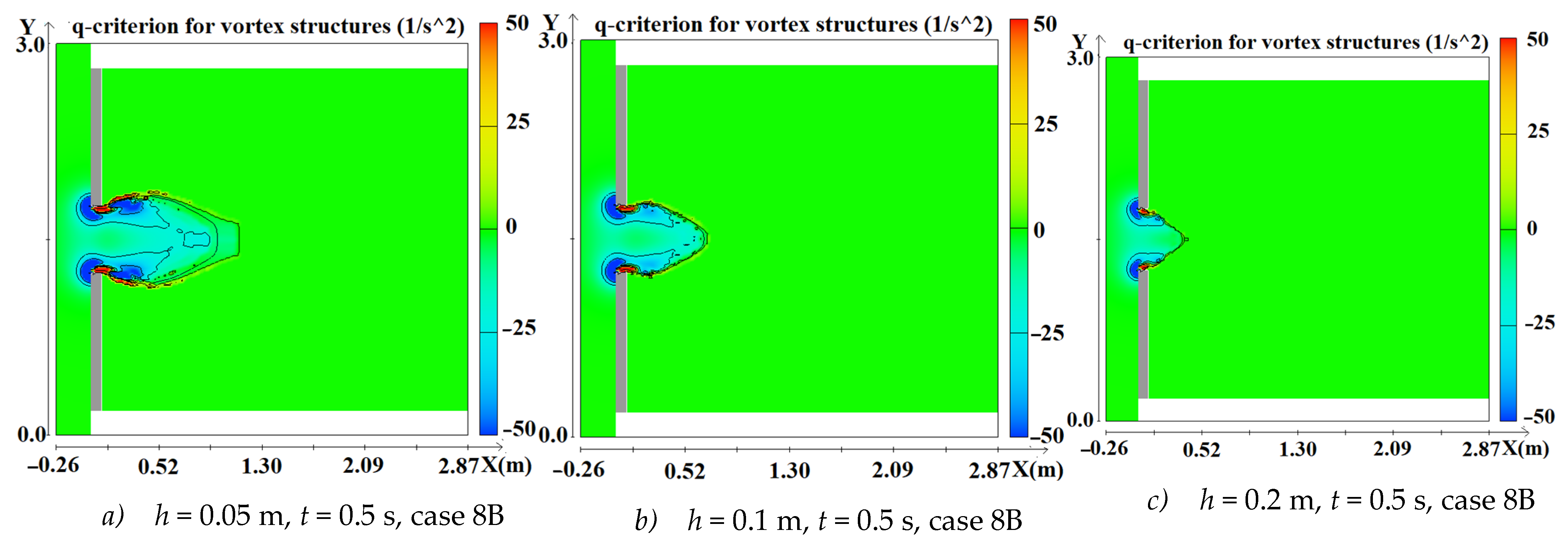
3.2.1. Dynamics and Structure of Dam–Break Wave Inside Reservoir

Eighteen different models are implemented to numerically investigate the effect of position of dam breach and its width (b) or breach ratio (b/B, where B is total length of dam) and initial water depth (h₀) on hydraulic characteristics of both rarefaction and shock waves (

Table 3. Case study.

Case	Initial Water Level (h0) (cm)	Opening Width (b) (cm) and b/B	Dam Gate Position
			A	B
1	20	25 (0.083)	Asymmetric	Centrer of dam
2	20	50 (0.166)	Asymmetric	Centrer of dam
3	20	75 (0.249)	Asymmetric	Centrer of dam
4	40	25 (0.083)	Asymmetric	Centrer of dam
5	40	50 (0.166)	Asymmetric	Centrer of dam
6	40	75 (0.249)	Asymmetric	Centrer of dam
7	60	25 (0.083)	Asymmetric	Centrer of dam
8	60	50 (0.166)	Asymmetric	Centrer of dam
9	60	75 (0.249)	Asymmetric	Centrer of dam

). Initial stage h₀ at the reservoir are taken as 20 cm, 40 cm and 60 cm, respectively, while downstream is dry. Two positions of reservoir outlet, asymmetrical (A) and symmetrical (B) with the central line of the dam, are involved.

To carry out the formation and structure of a rarefaction wave on the reservoir, 6 cases, 7A, 7B, 8A, 8B, 9A, 9B, corresponding with h₀ = 60 cm, are selected. The simulation time for all models was about 2 h of total dam–break time of 5.0 s, exceeding 3.02 million cells.

Streamlines show the direction of fluid elements that will travel assuming the flow at that point in time is steady [33]. The sudden overturning of reservoir water led to the formation and propagation of the rarefaction wave on water shortage and shock wave at the flood plain (Figure 4 and Figure 5). The free surface oscillates slightly within the reservoir in the early stage. In turn, the wave front velocity is increased by increasing breach size, because kinetic energy dissipation increases at the dam site in early–stage t = 0.5 s. In case B, streamline is performed symmetrically (see Figure 4), while the result in Figure 5 affirms the strong asymmetrical streamline, due to the effect of asymmetric location of the dam gate. Moreover, when t = 2.0 s, return flow within the reservoir is split into two parts, the small part goes to both the upper and lower corners of the reservoir and the larger one goes through the mouth of the reservoir in all cases 7B, 8B, 9B. At the same time, a small portion of water volume travels along the upstream bank of the reservoir and the larger one goes through the tank’s outlet in all models 7A, 8A, 9A. Later on, at t = 4.0s, all fluid elements within the reservoir move on towards the tank’s outlet, while the wetted area at flood plain generated by the smallest gate’s width is the largest (Figure 5).

Figure 6 and Figure 7 present water depth and velocity profiles at the center of the reservoir’s mouth when t = 1.5 s. The dam–break wave propagation is reduced by decreased breach width b and depends slightly on location of dam gate (Figure 6). Conversely, the wave front of velocity downstream decreases from b = 0.25 m to b = 0.75 m, and is independent of the reservoir outlet’s position. The numerical result of depth–averaged velocity gets its maximum value at x = 1.0 m in both 7A and 7B, then is gradually disregarded. While the value generated by larger breach size increases near the dam site and remains constant for the rest of the floodable area. On the other hand, the intersection point of three water depth profiles is after the dam site’s place in both cases of dam gate’s location, while the conjunction of 3 velocity profiles is placed at x = 0.

Transverse v velocity symmetrically distributes at the cross section near reservoir outlet in the 3 models 7B, 8B, 9B (Figure 8). In addition, when breach size increases, the highest value of near–bed v velocity increases and its position is further than the central line of the dam, because kinetic energy dissipation increases at the dam gate. In contrast, the 3 models 7A, 8A and 9A witness these values at the larger part of the reservoir, because a portion of the reservoir’s water moves to the reservoir’s outlet, unlike models 7B, 8B, 9B. Hence, with the same breach width, maximum transverse v–velocity of cases A are greater than those of cases B (Figure 8).

The dominant difference of water depth probes at the dam gate’s center yielded by the 6 scenarios is at normal peak points (Figure 9). Symmetrical dam breach provides a higher peak value of water depth than the asymmetrical one, although the lowest value of hump is independent of this factor. When breach size increases, the gradient of the water surface hydrograph increases.

Besides temporal variation of near–bed velocity, components u and w at the center of the outlet do not depend on the dam gate’s position, (Figure 10). In x direction, gate width b = 25 cm generates the maximum horizontal u velocity of 2 m/s, while the larger breach sizes, 50 cm and 75 cm, produce smaller values. Vertical component w is negative and nearly dismissed in all simulated times. This point is different with [28] when 4 breach sizes showed both negative and positive values of w. The reason may be due to the small ratio range b/B, from 0.08 to 0.25, in comparison with the larger range of (0.3 ÷ 1.0) in the aforementioned work. Additionally, transverse velocity v approximately equals zero when the reservoir’s mouth is symmetrical, while the harmonic trend of this value is seen in models 7A, 8A and 9A.

Vorticity components w_x, w_y, w_z represent the rate at which a fluid element rotates around its pivot axis [28]. The major effect of the opening gate’s location is observed in both values w_x and w_z. Negative value of horizontal vorticity w_x and positive value of vertical vorticity w_z present counterclockwise and clockwise rotations in models 7A, 8A and 9A during dam–beak time (Figure 11). While these values are negligible, due to the symmetrical dam’s mouth, it means there is no rotational flow formed in both x and z directions. Conversely, regarding time variation, clockwise w_y vorticity slightly depends on the position of the dam gate in the first 5 s period, except at the end of this period. Magnitude of w_y increases rapidly from b = 25 cm to b = 75 cm.

Vortex cores are centers of swirling flow where the velocity is parallel to the vorticity [33]. This parameter is very effective in identifying local rotational flow structures. The f_x–vortex core represents centers of swirling flow around pivot x axis. Figure 12 illustrates this index at t = 1.5 s in 6 cases 7A, 8A, 9A and 7B, 8B, 9B and shows that swirling flow occurs at the left side of the reservoir, which is near the mouth of the dam in all asymmetrical dam gate cases. When the opening width is larger, vortex core strength is greater. In contrast, the opposite trend occurs in the symmetrical dam gate. Swirling flow is indicated at two corners near the cross section of the dam, but its area is smaller when dam width is larger.

The quantity “q– criterion” represents the local balance between shear strain rate and vorticity magnitude, defining vortices as areas where the vorticity magnitude is greater than the magnitude of rate of strain, if q is greater than 0. The expression of q–criterion is [33]:

$$q_{criterion}=w_x^2+w_y^2+w_z^2-\frac{1}{2}{e}_{i,j}{e}_{i,j}$$

(6)

where:$e_{i,j}=\frac{1}{2}\left(\frac{\partial u_i}{\partial x_j}+\frac{\partial u_j}{\partial x_i}\right)$

As can be seen from Figure 13, the value of near–bed q–criterion at the center of the dam gate is counterclockwise in all cases 7A, 7B, 8A, 8B, 9A, 9B, in all computational times. The larger the opening width is, the greater the q–criterion gets. Regarding the largest breach width, the q value is clockwise, since t > 0.6 occurs in both positions of the dam gate. This means that light swirling flow occurs at the dam mouth at an early stage of dam–break flow. In addition, vortex flow in case 9A appears more clearly in time than that of 9B, which seems to grow fast at the end of the first 5 s of dam–break flow. The q value is 9.11 1/s² and 1.62 1/s² for former and latter, respectively. On the other hand, Figure 14 indicates minor differences in q–criterion contour maps between models 8A and 8B. The largest area of negative value appears at two sizes of dam gate, which means swirling flow occurs strongly at these positions. However, when water depth increases, these areas reduce and nearly vanish near free surface (Figure 15). So, vorticity occurs more strongly at the near–bed of the dam gate’s position than at near surface.

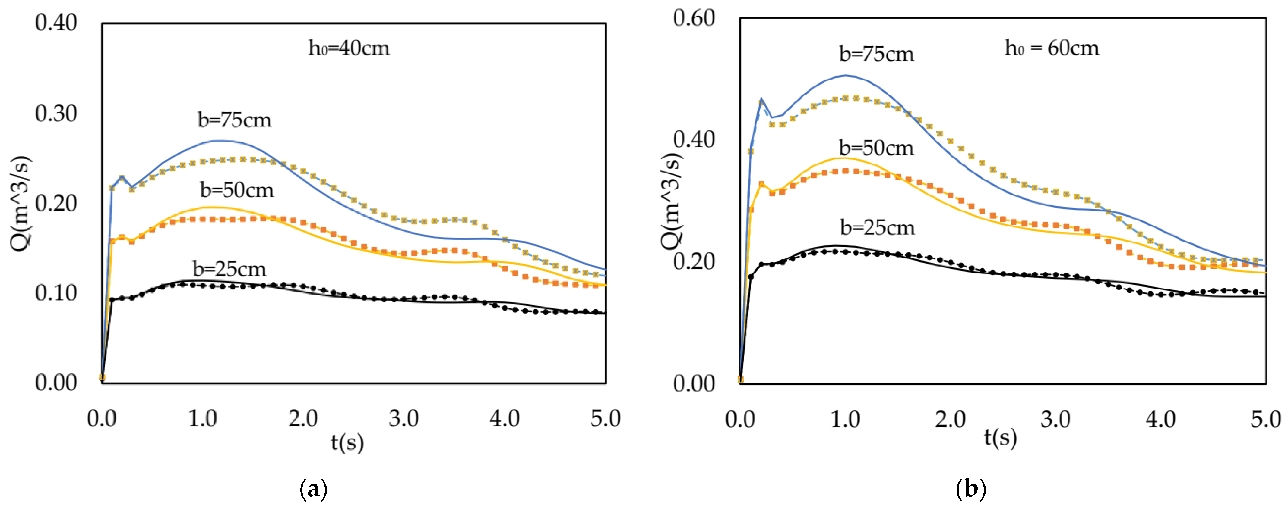
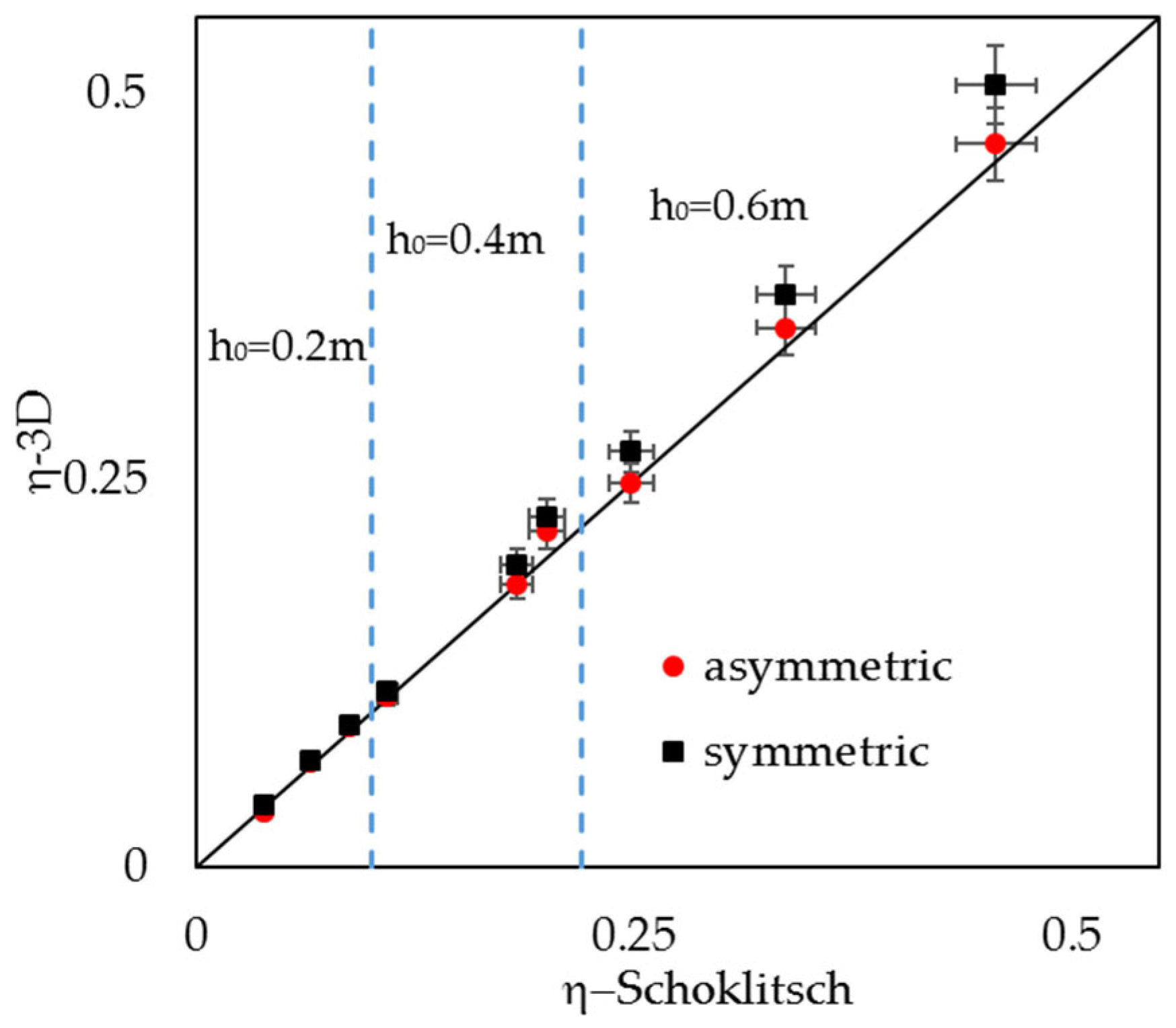
3.2.2. Peak Discharge of Outflow Hydrograph

In this section, peak discharge at dam site, produced by 18 models of partial dam collapse indicated in Table 3, is carefully investigated using the presented 3D CFD model.

Both the spike–shaped impulsive peak and the long–duration normal one are observed when breach size is enlarged (Figure 16). The latter is more significant than the former. This point shows an opposite conclusion to that of total dam collapse mentioned in [10]. The larger the breach size is, the greater the peak discharge generated. Moreover, regarding dam gate locations A or B, the significant difference between peak discharge values yielded by case A and case B is larger when broken width is greater. This point can be explained by water depth and u velocity profiles in Figure 9 and Figure 10, because discharge is an integral production of water depth and u velocity. Although minor change occurs between the two time series of u velocity of cases A and B (Figure 10), the major difference between the peaks of water depth yielded by cases A and B (Figure 9) causes dominant differences between peak flow rates.

Schoklitsch (1917) proposed an empirical equation to predict peak discharge in cases of full depth partial width breaches in rectangular channels [11]:

$$\frac{Q_p}{b\sqrt{g}{h}_o^{3/2}}={\left(\frac{8}{27}\right)}^{b/B}$$

(7)

Table 4. Peak discharge.

N°	h0 (cm)	b/B (–)	η–Schoklitsch (–)	η–3D, A (–)	η–3D, B (–)
1	20	0.084	0.5505	0.5140	0.5720
2	20	0.168	0.4629	0.4899	0.4924
3	20	0.251	0.4183	0.4363	0.4379
4	40	0.084	0.5505	0.5568	0.5785
5	40	0.168	0.4629	0.4626	0.4947
6	40	0.251	0.4183	0.4185	0.4531
7	60	0.084	0.5505	0.5975	0.6239
8	60	0.168	0.4629	0.4801	0.5095
9	60	0.251	0.4183	0.4291	0.4638

shows the dependence of ratio $\eta =\frac{Q_p}{b\sqrt{g}{h}_o^{3/2}}$ with b/B and initial water depth h₀ (m); Q_p (m³/s) is peak discharge. The range of b/B in this study is from 0.08 to 0.25, which has rarely been studied in previous literature. When h₀ remains constant, η calculated by Schoklitsch’s formula is also constant. However, this value is varied and increased when water stage increased. Most numerical results are greater than the analytical solution of Schoklitsch (1917) and symmetrical location of dam gate gives values of η greater than the asymmetrical one. Ascending initial water stage is, significantly, the difference between η–_Schoklitsch and η–_3D,_B. Regarding breach width b = 75 cm, 4.6%, 8.3% and 10.8% are the absolute error of η–_Schoklitsch and η–_3D,B corresponding with 3 values of water depth 20 cm, 40 cm and 60 cm, respectively. The scatter plot of comparison between peak discharge of models A and models B, with the analytical result of Schoklitsch, is reported in Figure 17. The former is closer with a diagonal line, than the latter, and all of them are greater than the analytical solution. Therefore, the VOF–LES model is straightforward in exactly capturing 3D hydraulic features of dam–break wave propagation.

4. Conclusions

In this research, the partial dam–break problem with symmetrical and asymmetrical locations of dam gate is exhibited accurately by the VOF–LES model. The effectiveness and robustness of the employed model in performing hydraulic characteristics within reservoirs and flood plains are achieved by using a reference test case from literature. The very good matching between predicted results of water depth, velocity component profiles and flooding map and observed results demonstrate that the presented 3D CFD model precisely predicts discontinuous, turbulent flow.

With a variety of initial stages and breach sizes, as well as two locations of partial dam failure, in 18 models, some novel numerical investigations of dam–break flow in early stage were discovered in this research and are listed below:

-

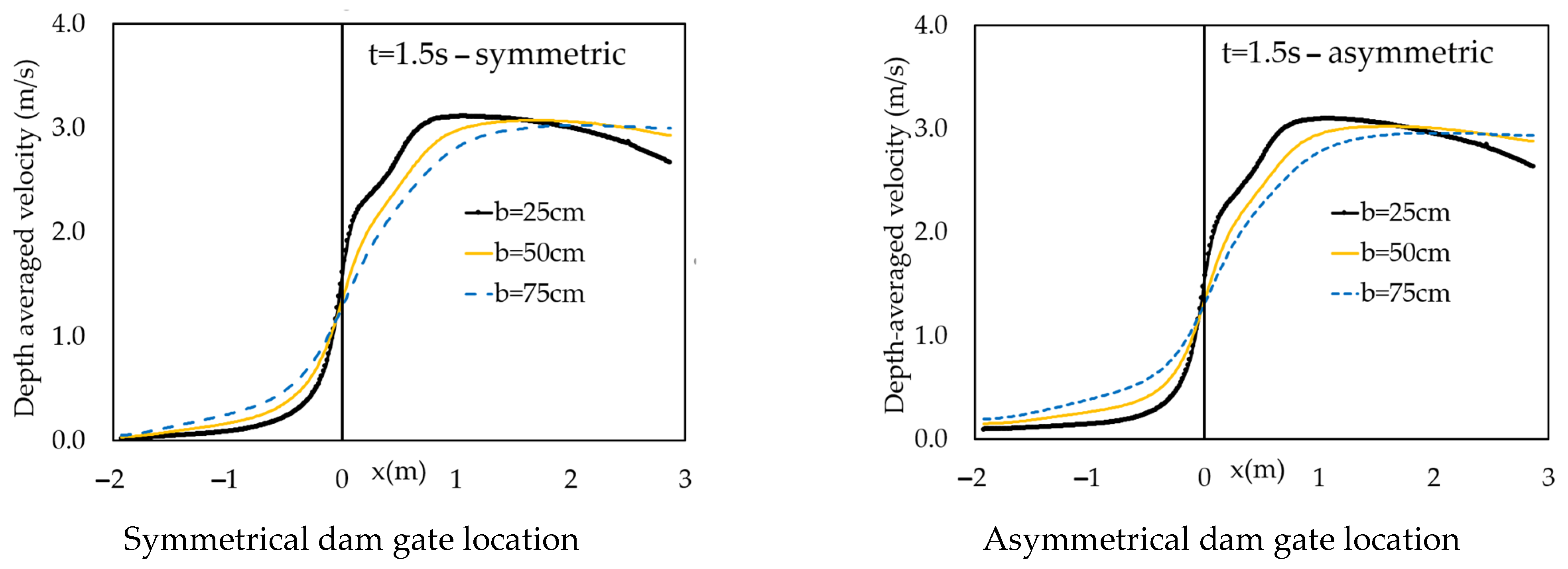
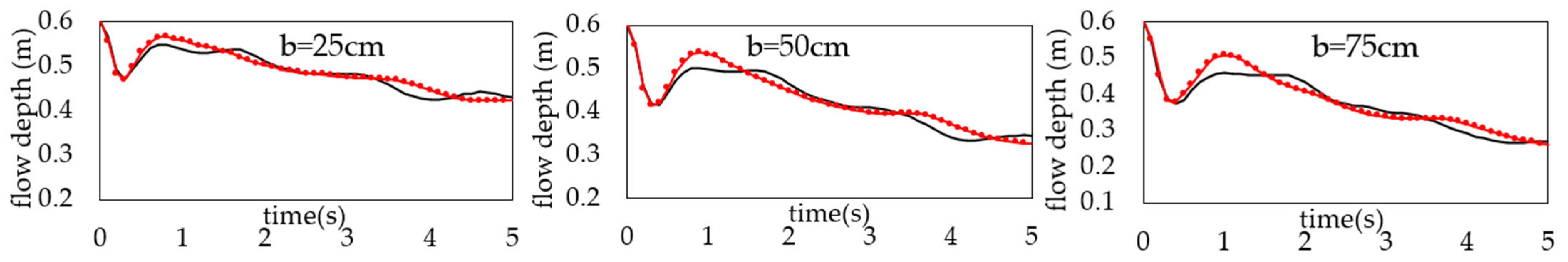
Increasing breach size causes reducing water depth profile at the central line of the dam gate on a reservoir. The opposite trend is observed in depth–average velocity hydrographs.

-

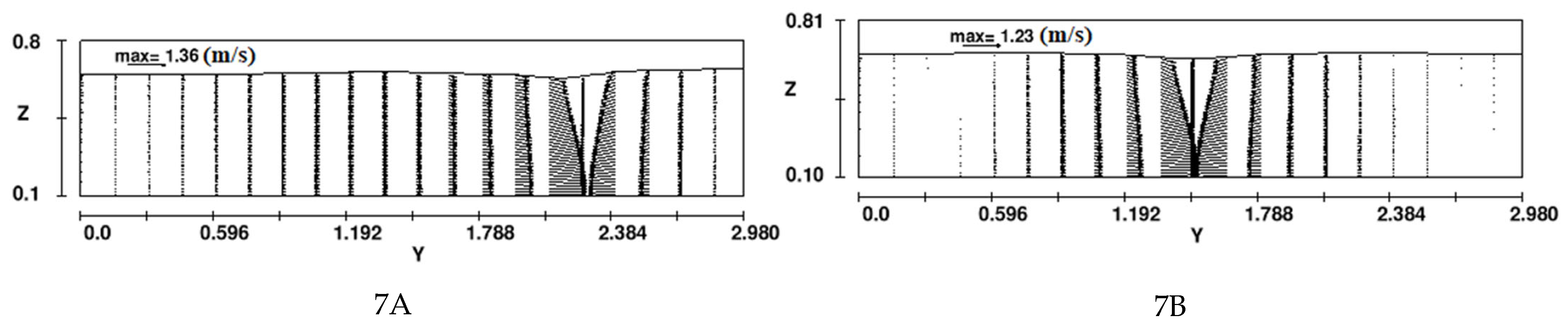
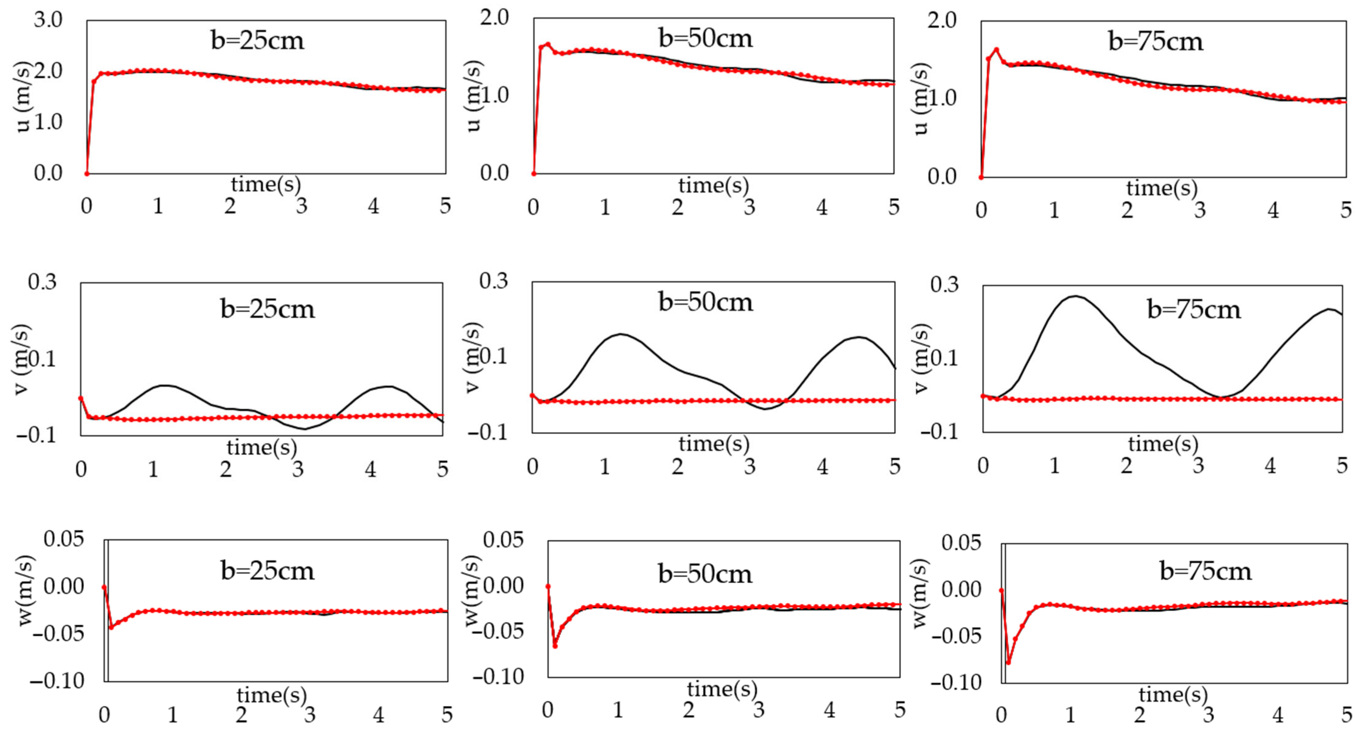
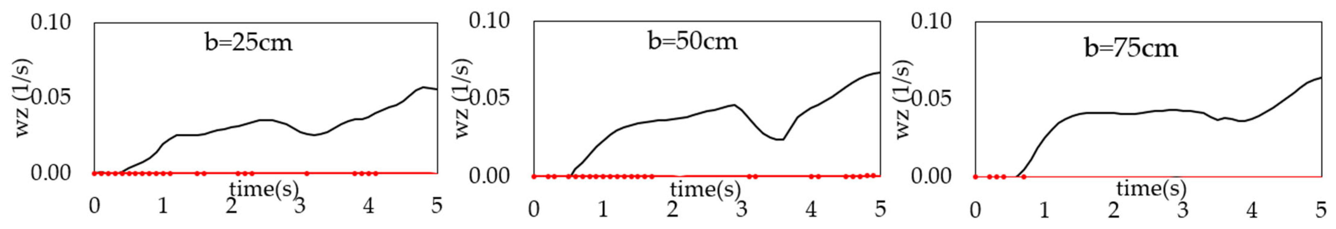
Velocity and vorticity components in x and z directions are independent of the position of dam gate. In contrast, components v and w_y in the y axis vanished when the reservoir outlet was at the central line of the dam.

-

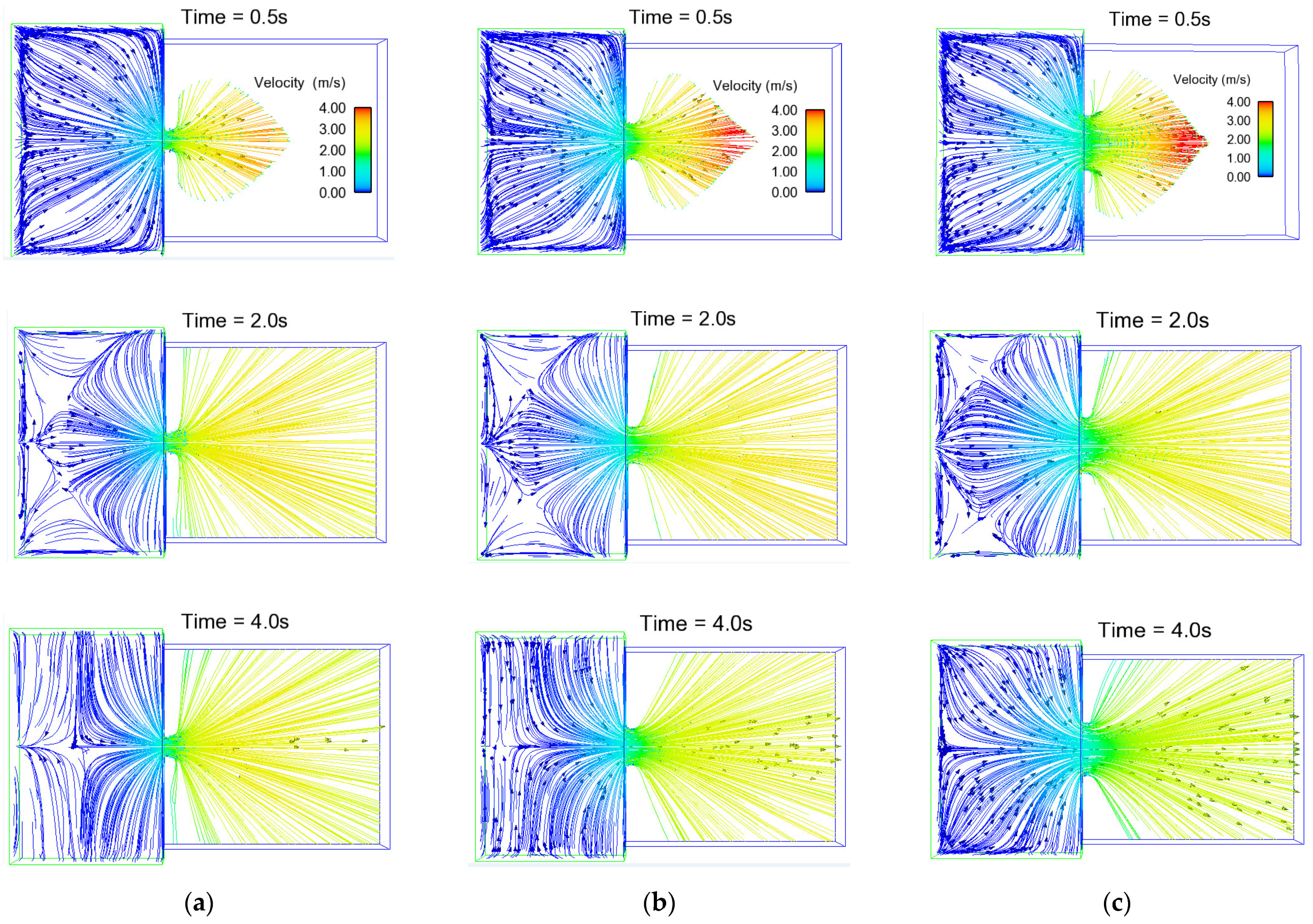
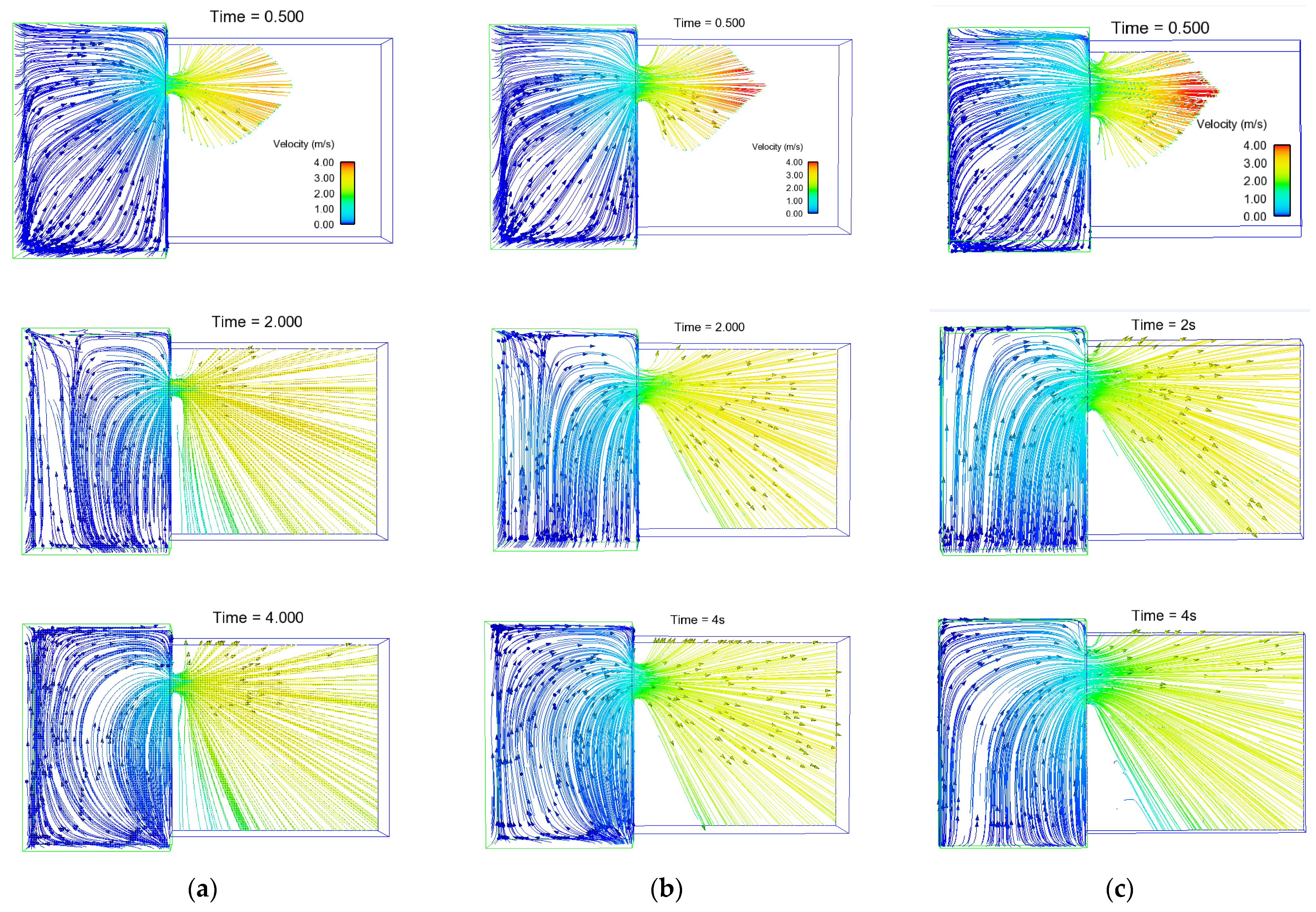
Streamline patterns exhibit the movement of fluid particles at certain times. In early stage, not all fluid elements move to the reservoir mouth when breach size is small.

-

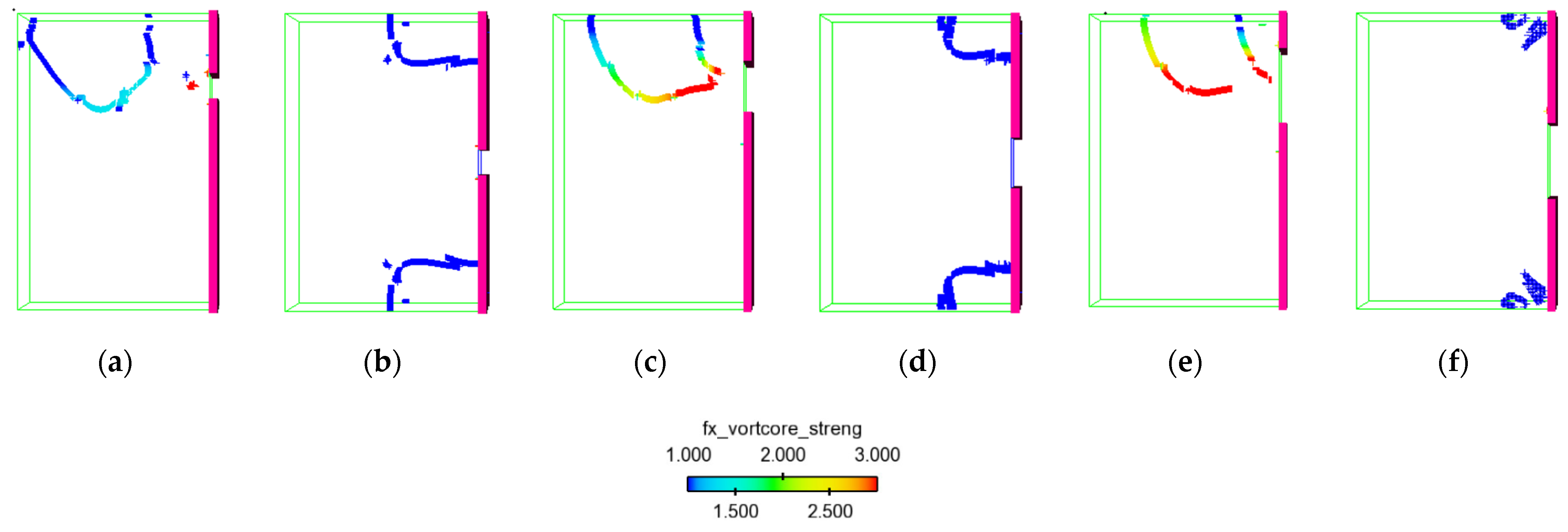
Some sophisticated hydraulic factors indicating swirling flow are involved in the time series of q–criterion and vortex core mapping. In the case of symmetrical reservoir outlet, breach width increases, vortex core area at both corners near the dam site decreases, which means vorticity is weak. In contrast, stronger swirling flow appeared near the top right corner of the reservoir when a broken block is asymmetrically placed.

-

Normal peak discharge does not only depend on initial water stage, and dam breach ratio. It is also influenced by location of dam gate. The reservoir’s initial water stage is greater, and maximum flow rate released by symmetrical breach location is more notable, than those released by the asymmetrical case.

The selected model indicated high accuracy and clarity in performing several 3D hydraulic characteristics of partial dam–break flow. It is also extremely straightforward in providing a wide range of options for geometry of computational domain and initial conditions.

References

1. Fraccarollo, L.; Toro, E.F. Experimental and numerical assessment of the shallow water model for two–dimensional dam–break type problems. J. Hydraul. Res. 1995, 33, 843–864. [Google Scholar] [CrossRef]
2. Aureli, F.; Mignosa, P.; Tomirotti, M. Numerical simulation and experimental verification of Dam–Break flows with shocks. J. Hydraul. Res. 2000, 38, 197–206. [Google Scholar] [CrossRef]
3. Proust, S.; Berni, C.; Boudou, M.; Chiaverini, A.; Dupuis, V.; André, J.-B.F.; Paquier, M.L.; Guillen–Ludena, S.; Lopez, D. Predicting the flow in the floodplains with evolving land occupations during extreme flood events (FlowRes ANR project). E3S Web Conf. 2016, 7, 04004. [Google Scholar] [CrossRef] [Green Version]
4. Aureli, F.; Maranzoni, A.; Mignosa, P.; Ziveri, C. Dam–Break Flows: Acquisition of Experimental Data through an Imaging Technique and 2D Numerical Modeling. J. Hydraul. Eng. 2008, 134, 1089–1101. [Google Scholar] [CrossRef]
5. Aureli, F.; Maranzoni, A.; Mignosa, P.; Ziveri, C. An image processing technique for measuring free surface of dam–break flows. Exp. Fluids 2010, 50, 665–675. [Google Scholar] [CrossRef]
6. Aureli, F.; Maranzoni, A.; Mignosa, P. A semi–analytical method for predicting the outflow hydrograph due to dam–break in natural valleys. Adv. Water Resour. 2014, 63, 38–44. [Google Scholar] [CrossRef]
7. Soares–Frazão, S.; Zech, Y. Experimental study of dam–break flow against an isolated obstacle. J. Hydraul. Res. 2007, 45, 27–36. [Google Scholar] [CrossRef]
8. Soares–Frazão, S.; Zech, Y. Dam–break flow through an idealised city. J. Hydraul. Res. 2008, 46, 648–658. [Google Scholar] [CrossRef] [Green Version]
9. Lobovský, L.; Botia–Vera, E.; Castellana, F.; Mas–Soler, J.; Souto–Iglesias, A. Experimental investigation of dynamic pressure loads during dam–break. J. Fluids Struct. 2014, 48, 407–434. [Google Scholar] [CrossRef] [Green Version]
10. Liu, S.; Liu, H. An experimental study of the maximum run–up height under dambreak flow on the initial dry–bed. J. Ocean Univ. China 2017, 16, 697–702. [Google Scholar] [CrossRef]
11. Schoklitsch, A. On waves created by dam breaches (in German). Sitz. Der Kais. Akad. Der Wiss. Wien 1917, 126, 1489–1514. [Google Scholar]
12. Waterway Experiment Station (WES). Floods resulting from suddenly breached dams. Misc paper no 2–374. Rep 1: Conditions of minimum resistance. Rep. prepared for U.S. Army Corps of Engineers, Vicksburg, MS, USA, 1960. [Google Scholar]
13. Zhang, X.; Pirker, S.; Saeedipour, M. Numerical investigation of particle motion at the steel—slag interface in continuous casting using VOF method and dynamic overset grids. Exp. Comput. Multiph. Flow 2022, 1–14. [Google Scholar] [CrossRef]
14. Zhang, H.; Li, Y.; Xiao, J.; Jordan, T. Large eddy simulation of turbulent flow using the parallel computational fluid dynamics code GASFLOW–MPI. Nucl. Eng. Technol. 2017, 49, 1310–1317. [Google Scholar] [CrossRef]
15. Yu, S.; Lim, J.; Cho, I.; Han, J. Inerting Strategy for a Demonstration–Scale Hot Cell Facility Based on Experiences from Pilot–Scale Argon Cell Facility Operation and CFD Analysis. Sci. Technol. Nucl. Install. 2021, 2021, 1–12. [Google Scholar] [CrossRef]
16. Shige–eda, M.; Akiyama, J. Numerical and Experimental Study on Two–Dimensional Flood Flows with and without Structures. J. Hydraul. Eng. 2003, 129, 817–821. [Google Scholar] [CrossRef]
17. Khankandi, F.A.; Tahershamsi, A.; Soares–Frazão, S. Experimental investigation of reservoir geometry effect on dam–break flow. J. Hydraul. Res. 2012, 50, 376–387. [Google Scholar] [CrossRef]
18. Hiền, L.T.T.; Hiền, N.T. Đánh giá ảnh hưởng của dòng chảy vỡ đập khi có và không có vật cản bằng mô hình toán hai chiều. processings of the Hội Nghị Cơ Học Thủy Khí Lần Thứ 21, Quy Nhon, Vietnam, 19–21 July 2018. (In Vietnamese). [Google Scholar]
19. Pilotti, M.; Tomirotti, M.; Valerio, G.; Bacchi, B. Simplified Method for the Characterization of the Hydrograph following a Sudden Partial Dam–break. J. Hydraul. Eng. 2010, 136, 693–704. [Google Scholar] [CrossRef]
20. Ozmen–Cagatay, H.; Kocaman, S. Dam–break flows during initial stage using SWE and RANS approaches. J. Hydraul. Res. 2010, 48, 603–611. [Google Scholar] [CrossRef]
21. Hien, L.T.T.; Van Chien, N. Investigate Impact Force of Dam–Break Flow against Structures by Both 2D and 3D Numerical Simulations. Water 2021, 13, 344. [Google Scholar] [CrossRef]
22. Aureli, F.; Dazzi, A.; Maranzoni, A.; Mignosa, P.; Vacondio, R. Experimental and numerical evaluation of the force due to the impact of a dam–break wave on a structure. Adv. Water Resour 2015, 76, 29–42. [Google Scholar] [CrossRef]
23. Larocque, L.A.; Imran, J.; Chaudhry, M.H. 3D numerical simulation of partial breach dam–break flow using the LES and k–ϵ turbulence models. J. Hydraul. Res. 2013, 51, 145–157. [Google Scholar] [CrossRef]
24. Biscarini, C.; Di Francesco, S.; Manciola, P. CFD modelling approach for dam–break flow studies. Hydrol. Earth Syst. Sci. Discuss. 2009, 6, 6759–6793. [Google Scholar] [CrossRef] [Green Version]
25. Yang, S.; Yang, W.; Qin, S.; Li, Q.; Yang, B. Numerical study on characteristics of dam–break wave. Ocean Eng. 2018, 159, 358–371. [Google Scholar] [CrossRef]
26. Saghi, H.; Lakzian, E. Effects of using obstacles on the dam–break flow based on entropy generation analysis. Eur. Phys. J. Plus 2019, 134, 237. [Google Scholar] [CrossRef]
27. Khoshkonesh, A.; Nsom, B.; Gohari, S.; Banejad, H. A comprehensive study on dam–break flow over dry and wet beds. Ocean Eng. 2019, 188, 106279. [Google Scholar] [CrossRef]
28. Khoshkonesh, A.; Nsom, B.; Bahmanpouri, F.; Dehrashid, F.A.; Adeli, A. Numerical Study of the Dynamics and Structure of a Partial Dam–Break Flow Using the VOF Method. Water Resour. Manag. 2021, 35, 1513–1528. [Google Scholar] [CrossRef]
29. Hu, H.; Zhang, J.; Li, T.; Yang, J. A simplified mathematical model for the dam–breach hydrograph for three reservoir geometries following a sudden full dam–break. Nat. Hazards 2020, 102.3, 1515–1540. [Google Scholar] [CrossRef]
30. Tsakiris, G.; Spiliotis, M. Dam– Breach Hydrograph Modelling: An Innovative Semi– Analytical Approach. Water Resour. Manag. 2012, 27, 1751–1762. [Google Scholar] [CrossRef]
31. Kaurav, R.; Mohapatra, P.K. Studying the Peak Discharge through a Planar Dam Breach. J. Hydraul. Eng. 2019, 145, 06019010. [Google Scholar] [CrossRef]
32. Lee, K.-H. Simulation of Dam–Breach Outflow Hydrographs Using Water Level Variations. Water Resour. Manag. 2019, 33, 3781–3797. [Google Scholar] [CrossRef]
33. Flow–3D; Version 12.0; User Manual; Flow Science Inc.: Santa Fe, NM, USA, 2020.
34. Hirt, C.; Nichols, B. Volume of fluid (VOF) method for the dynamics of free boundaries. Journal of Computational Physics. 1985, 39(1), 201–225. [Google Scholar] [CrossRef]
35. Ketabdari, M.J.; Saghi, H. Large Eddy Simulation of Laminar and Turbulent Flow on Collocated and Staggered Grids. ISRN Mech. Eng. 2011, 2011, 1–13. [Google Scholar] [CrossRef] [Green Version]
36. Smagorinsky, J. General circulation experiments with the primitive equations. Mon. Wea. Rev. 1963, 91, 99–164. [Google Scholar] [CrossRef]
Figure 1. Configuration of experimental model.
Applsci 12 03884 g001
Figure 2. Water depth profiles at different gauges.
Applsci 12 03884 g002aApplsci 12 03884 g002b
Figure 3. Flood extent at downstream. (a) t = 0.50 s, (b) t = 0.77 s, (c) t = 1.50 s.
Applsci 12 03884 g003
Figure 4. Streamline of magnitude velocity at different time in 3 models: (a) 7B, (b) 8B, (c) 9B.
Applsci 12 03884 g004
Figure 5. Streamline of magnitude velocity at different time in 3 models: (a) 7A, (b) 8A, (c) 9A.
Applsci 12 03884 g005
Figure 6. Water depth profiles at central axis of partial dam collapsed.
Applsci 12 03884 g006
Figure 7. Depth–average velocity profiles at central line of dam gate at t = 1.5 s.
Applsci 12 03884 g007
Figure 8. Distribution of transverse v velocity near dam site at t = 1.5 s.
Applsci 12 03884 g008aApplsci 12 03884 g008b
Figure 9. Water depth profiles at the center of dam gate. Solid line: cases 7A, 8A, 9A; dot line: cases 7B, 8B, 9B.
Applsci 12 03884 g009
Figure 10. Near–bed velocity component profiles at the center of dam gate. Black solid line—asymmetrical dam gate; Red dotted line—symmetrical dam gate.
Applsci 12 03884 g010
Figure 11. Near−bed vorticity components at the center of dam site. Black solid line: cases 7A, 8A, 9A; red dotted line: cases 7B, 8B, 9B.
Applsci 12 03884 g011aApplsci 12 03884 g011b
Figure 12. fx–vortex core strength at early stage of dam breach at t = 1.5 s. (a) 7A, (b) 7B, (c) 8A, (d) 8B, (e) 9A, (f) 9B.
Applsci 12 03884 g012
Figure 13. Near–bed q–criterion at the center of dam gate. Solid line–asymmetrical dam gate; dot line–symmetrical one.
Applsci 12 03884 g013
Figure 14. Near−bed iso−surface map of q−criterion at t = 0.5 s and t = 2.0 s in cases 8A and 8B.
Applsci 12 03884 g014
Figure 15. Contour maps of q−criterion at t = 0.5 s at different water depths.
Applsci 12 03884 g015
Figure 16. Discharge hydrographs taken with output interval 0.1 s. Solid line–cases B. Marker line–cases A. (a) h0 = 40 cm, (b) h0 = 60 cm.
Applsci 12 03884 g016
Figure 17. Comparison between analytical results with numerical ones.
Applsci 12 03884 g017