Improved FULMS Algorithm for Multi-Modal Active Control of Compressor Vibration and Noise Reduction

Abstract

Active control is currently a hot-button issue in the research of reducing vibration and noise created by rolling piston compressors. Active control can effectively suppress the modal vibration of the structure and reduce the modal resonance acoustic radiation. This paper, which focuses on the active control of the compressor shell’s multiple modes with the control of acoustic radiation power being the research objective, studies the relationship between vibration modes and acoustic radiation modes of the compressor shell and the primary sources of noise. An improved Filtered-U least mean square (FULMS) algorithm for compressor vibration and noise control, which is based on the Nesterov accelerated adaptive moment estimation (NADAM) optimization algorithm, is proposed to determine the multi-order modes to be controlled from the perspective of sound energy, and a particle swarm algorithm is used to determine the location and number of secondary sources. The active control model of the compressor shell was established by using the joint simulation platform, and the performance of the improved algorithm was verified and analyzed by the simulation test process. The results show that compared with the traditional FULMS algorithm, the improved FULMS algorithm has better active vibration control effect, higher convergence speed and can effectively suppress structural mode vibration in a short period time.

1. Introduction

Rolling piston compressors, as the core component of the refrigeration system, are commonly used in refrigeration equipment, but they produce much noise while in operation. In recent years, scholars have carried out wide-ranging research on the flow of refrigerant in rolling piston compressor, structural mode vibration, and noise reduction technology. Some progress has been achieved [1,2,3,4]. However, in the operation of the roller piston compressor, there are multi-source excitations such as structural vibration excitation, fluid pulsation excitation and electromagnetic excitation as well as acoustic radiation of structural multi-mode coupling vibration [5]. Traditional passive noise control methods cannot satisfy noise reduction requirements. Through secondary source active control technology, structural vibration of the compressor shell can be suppressed, and acoustic radiation can be reduced.

Active vibration control is closely associated with the wave-filtering algorithms of self-adaptive filters. At present, the most widely used self-adaptive wave filtering algorithm is the Least Mean Squares (LMS) algorithm, which was originally proposed by Widrow [6] and promoted by Morgan [7] to be applied in situations where linear wave filtering appears in a closed circuit of auxiliary signals. As active control systems that utilize the LMS algorithm are mostly open-loop control, these active control systems encounter certain problems like signals with no feedback and the delay of secondary channels. Burgess [8] on the basis of LMS logarithm strengthened the evaluation of secondary channels to delay real-life signals and proposed the Filtered-X Least Mean Squares (FXLMS) algorithm. Saito et al. [9] studied the effect of the approximation errors during the modeling of secondary channels on the performance of the FXLMS algorithm. Douglas [10] invented the multi-HYPER channel algorithm to eliminate the problem of multi-channel control is too complicated and difficult to realize. Das [11] improved the structure of active noise control with Fast Fourier Transformation and Hartley Transform to downsize the calculation. To tackle the problem that the feedback of output signals were not considered in the FXLMS algorithm, Eriksson [12] proposed the Filtered-U Least Mean Squares (FULMS) algorithm. Kim [13] became the first person to apply the FULMS algorithm in engineering problems. FULMS was employed to conduct active noise control of pipes and effectively reduced the noise in the pipes. However, due to the acoustic feedback problem in the structure, the active control effect is reduced and becomes unstable. Turpati Suman [14] proposed and developed a Harmonic Mean Dependent Variable Step Size (HMVSS) method, which can effectively improve the convergence speed of active control in pipeline noise control and has a good noise reduction effect. Researchers have made numerous attempts to optimize stringency, stability, and applicability of active control algorithms, and the performance of those algorithms has been dramatically advanced and developed [15,16,17,18]. In the meantime, those algorithms have been applied to real-life engineering fields with significant achievements.

However, active vibration and noise control of objects with complex structures and irregular shapes still face essential challenges including optimized arrangement methods and controlling algorithms of sensors and actuators. Therefore, the novelty of this study is that the compressor structure is complex, and there are many excitation sources. Particularly noteworthy is that this paper, having rolling piston compressors as its research objective, studies the active control algorithm of the multiple modes of the compressor shell. The FULMS algorithm was optimized with the NADAM optimizer to enhance the efficiency and astringency of the algorithm. Finally, active control of the compressor shell was simulated. The algorithm was verified with experiments so as to determine the control effect and astringency of the improved algorithm on noise and vibration created by complex components.

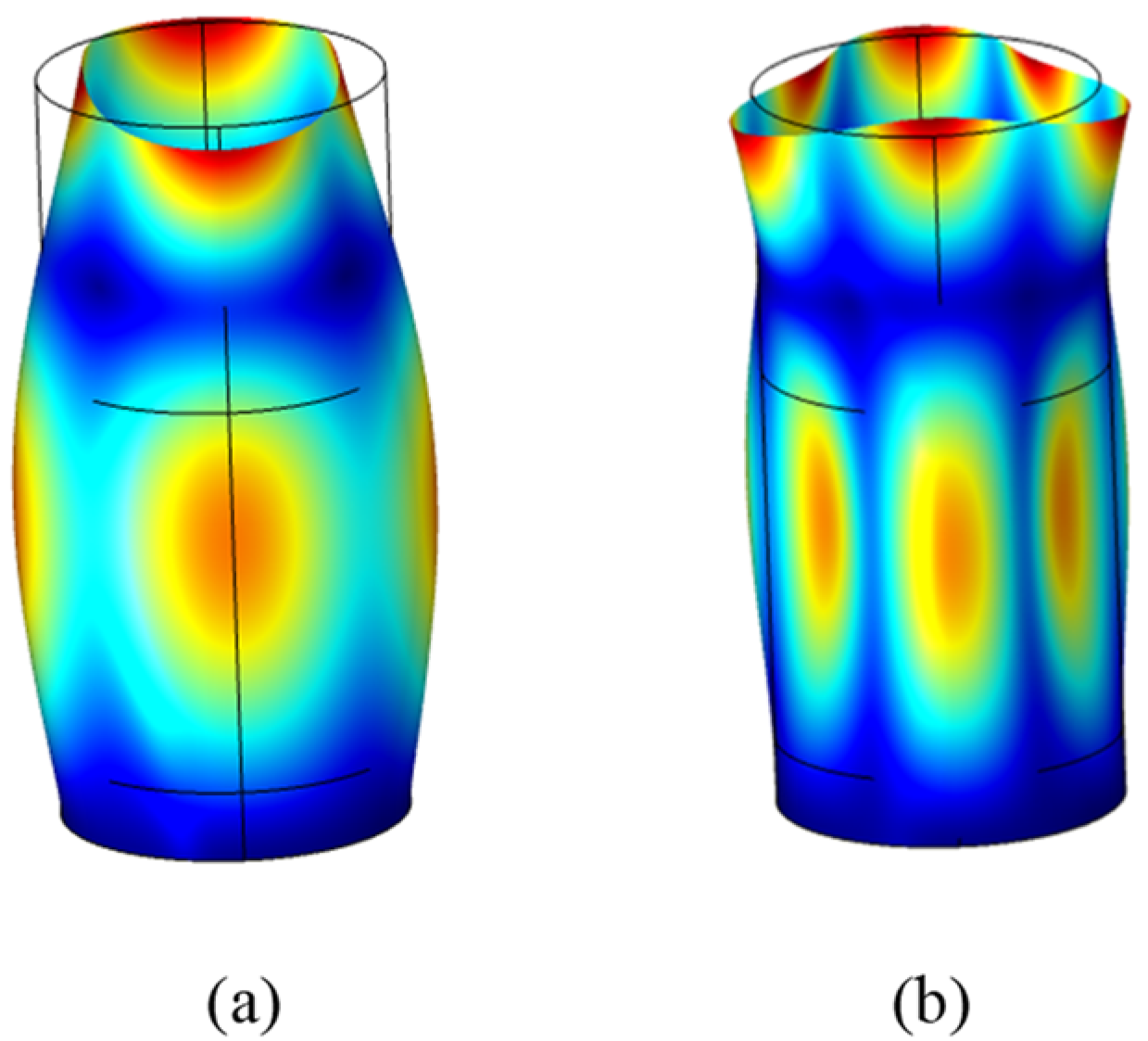
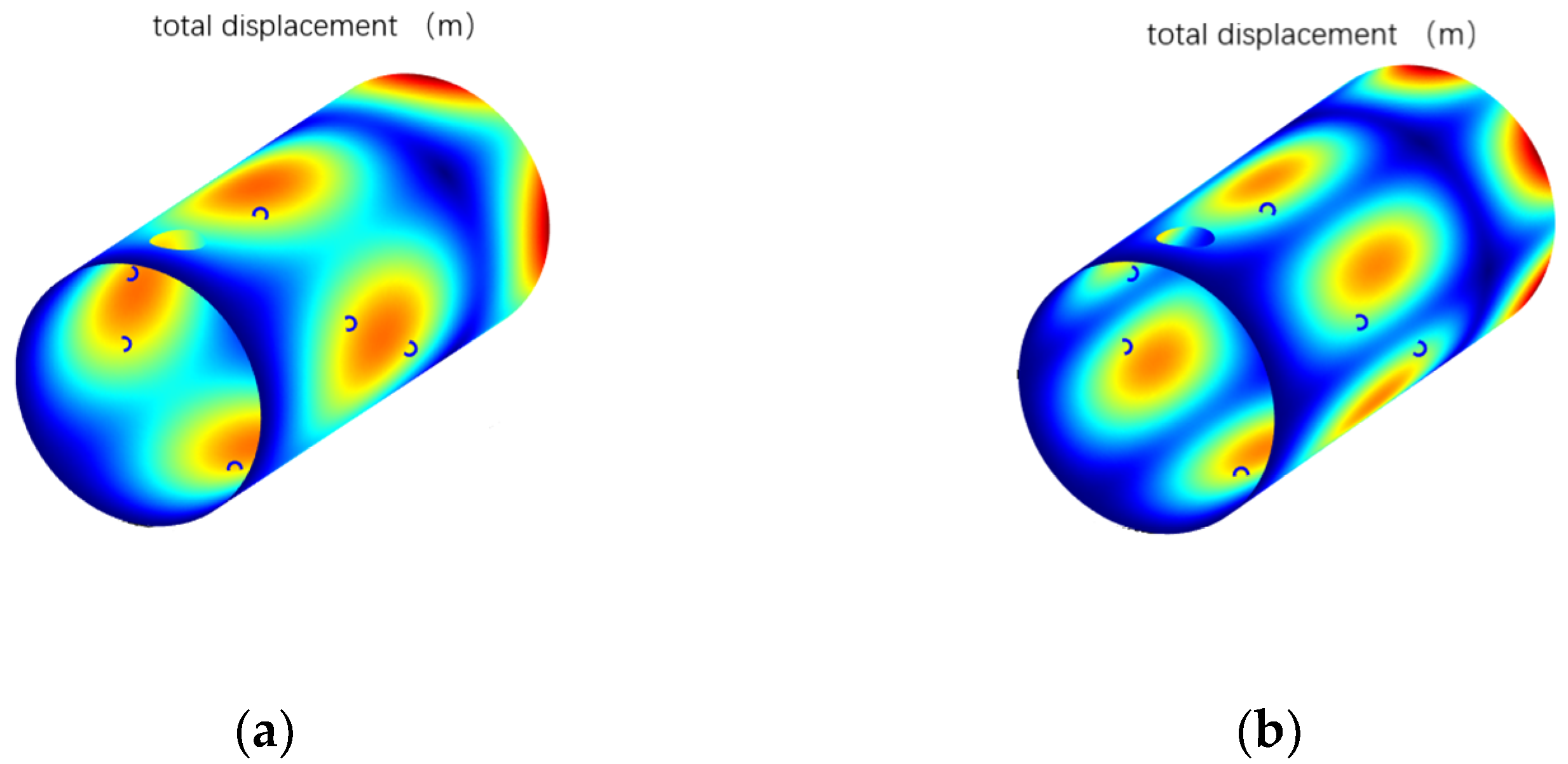
2. Modal Analysis of Vibration and Sound Radiation

Taking the undamped n-order degree of freedom system as an example, the differential equation of motion is as follows:

$$\left[m\right]\left\{\ddot{x}\left(t\right)\right\}+\left[k\right]\left\{x\left(t\right)\right\}=\left\{Q\left(t\right)\right\}$$

(1)

where $\left[m\right]$ and $\left[k\right]$ are the mass matrix and the stiffness matrix of each node respectively. $\left\{Q\left(t\right)\right\}$ is the excitation matrix. When the external force received by the system is a simple harmonic force, after decoupling and transformation of the equation, the steady-state response of the system can be calculated as follows:

$$\left\{x\left(t\right)\right\}={\displaystyle \sum }_{r=1}^n\left\{u^r\right\}\frac{N_{0r}/{\omega }_r^2}{\sqrt{1-{(\omega /{\omega }_r)}^2}}sin(\omega t)$$

(2)

among them, $\omega$ is the excitation frequency. ${\omega }_r$ is the r-th natural frequency, and $\left\{u^r\right\}$ is the r-th modal vector. It can be seen that when the excitation frequency is close to the r-th natural frequency, resonance occurs, and a large displacement response is generated. The vibration mode shape and energy frequency response of each mode can be obtained through model calculation to evaluate the active position and frequency band of vibration mode, respectively.

The acoustic radiation mode is generated during the derivation of acoustic radiation power. Taking the unit radiator method as an example, the following formula can be obtained:

$$W={(Q^{T}v)}^H\Lambda \left(Q^{T}v\right)=Y^H\Lambda Y={\displaystyle \sum }_{\mathrm{i}=1}{\lambda }_i{\left|y_i\right|}^2={\displaystyle \sum }_{\mathrm{i}=1}{W}_i$$

(3)

where $Q$ and $\Lambda$ are the characteristic matrix after eigenvalue decomposition of acoustic radiation resistance matrix and the diagonal matrix composed of eigenvalues, respectively. $v$ is the normal velocity vector of plane element. Formula (3) shows that the acoustic radiation on the structural surface is the superposition of each order of acoustic radiation modes [19], so the acoustic radiation of the structure can be reduced by suppressing the acoustic radiation modes.

According to the modal superposition principle, the radiated sound power of the structure can also be expressed as

$$\mathrm{W}= {\rho }_0{c}_{0}S{v}^2\sigma$$

(4)

where S is the area in the propagation direction, and v is the vibration velocity level of the structure, which can be calculated by the root mean square of the vibration velocity of the structure, and σ is the radiation efficiency. According to Equation (3) and the orthogonality of eigenvectors:

$${\sigma }_i=\frac{2{\lambda }_i}{({\rho }_0{c}_0)S}$$

(5)

among them, λ_i is the eigenvalue of the acoustic radiation resistance matrix. From Formula (5), σ_i is only related to the eigenvalue and radiation area of the acoustic radiation resistance matrix R. According to the physical meaning and transformation process of R, the radiation efficiency of the acoustic radiation mode is only determined by the geometric characteristics of the radiator and the excitation frequency [20].

The sound power of each order of the radiation mode is the product of radiation efficiency and modal amplitude. According to the radiation efficiency calculation formula, the modal radiation efficiency has no strong positive correlation with the amplitude of vibration mode, but the amplitude of the radiation mode is related to the vibration velocity. Through the analysis of the vibration mode, it is easy to know that the vibration velocity is the superposition of each order of vibration modes, so the relationship between them can be studied. The acoustic radiation mode is controlled by suppressing the vibration mode.

According to the analysis of the steady-state response of vibration, the velocity distribution of the vibrating part can be expressed as the superposition of the modes of each order, i.e.,

$$v={\displaystyle \sum }_{i=1}^N{A}_i{\Phi }_i$$

(6)

where N is the highest vibration mode order considered, A_i is the velocity amplitude of the i-th vibration mode, and Φ_i is the corresponding vibration mode distribution. Simultaneous Equations (3) and (6) can obtain

$$Y=Q^{T}v={\displaystyle \sum }_{i=1}^N{Q}^T{A}_i{\Phi }_i={\displaystyle \sum }_{j=1}^M{\displaystyle \sum }_{i=1}^N{q}_j^T{A}_i{\Phi }_i$$

(7)

In Formula (7), M is the highest acoustic radiation mode order considered, and q_j is the vibration mode of the j-th acoustic radiation mode, indicating that the vibration mode affects the amplitude of the acoustic radiation mode. According to the calculation formula of sound radiation power, the vibration mode can affect the sound power by affecting the amplitude of sound radiation mode. Therefore, after determining the control frequency band and excitation source, the vibration mode of the corresponding frequency band can be suppressed through active control to reduce the sound radiation power and achieve the effect of vibration and noise reduction.

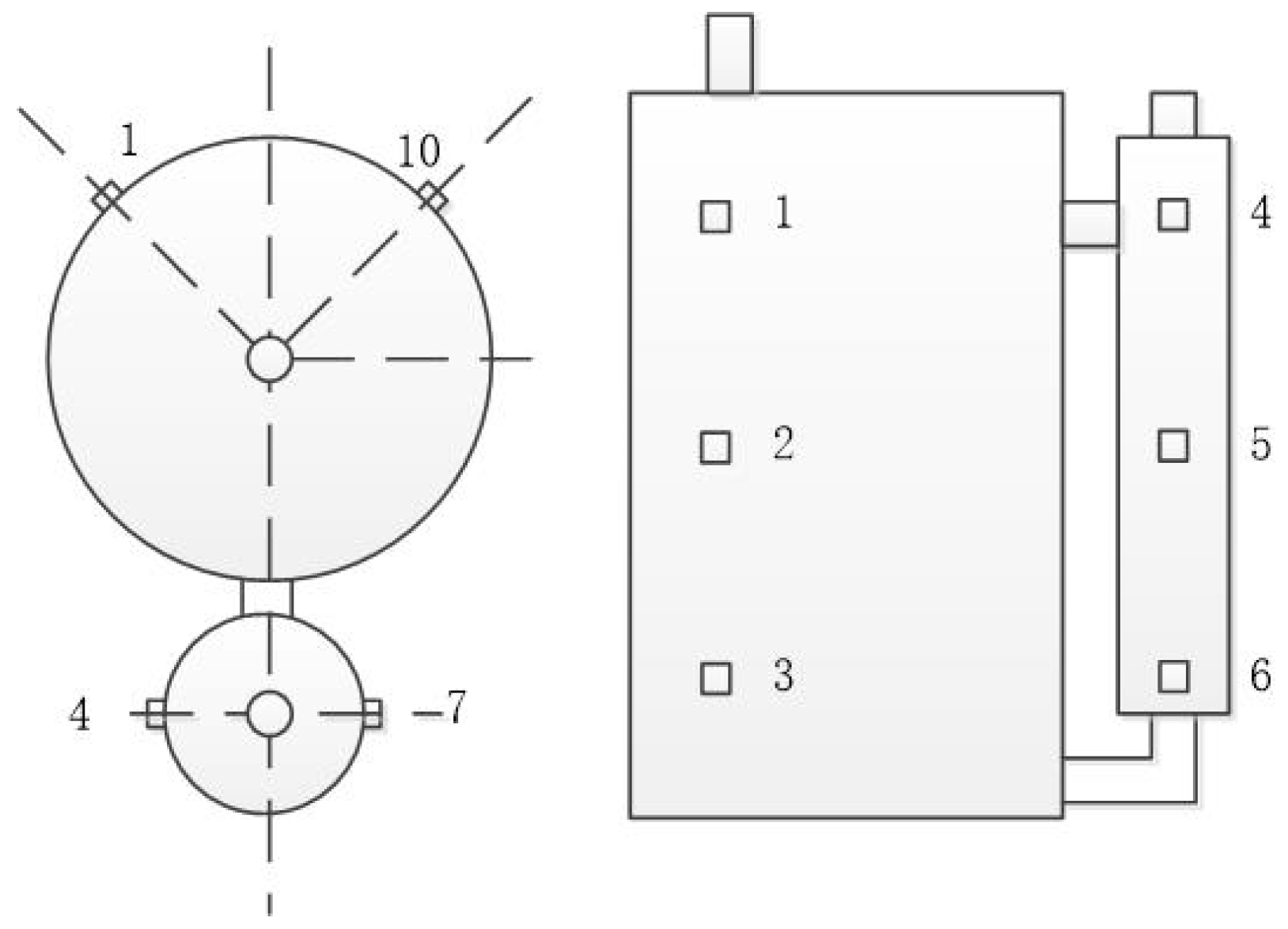
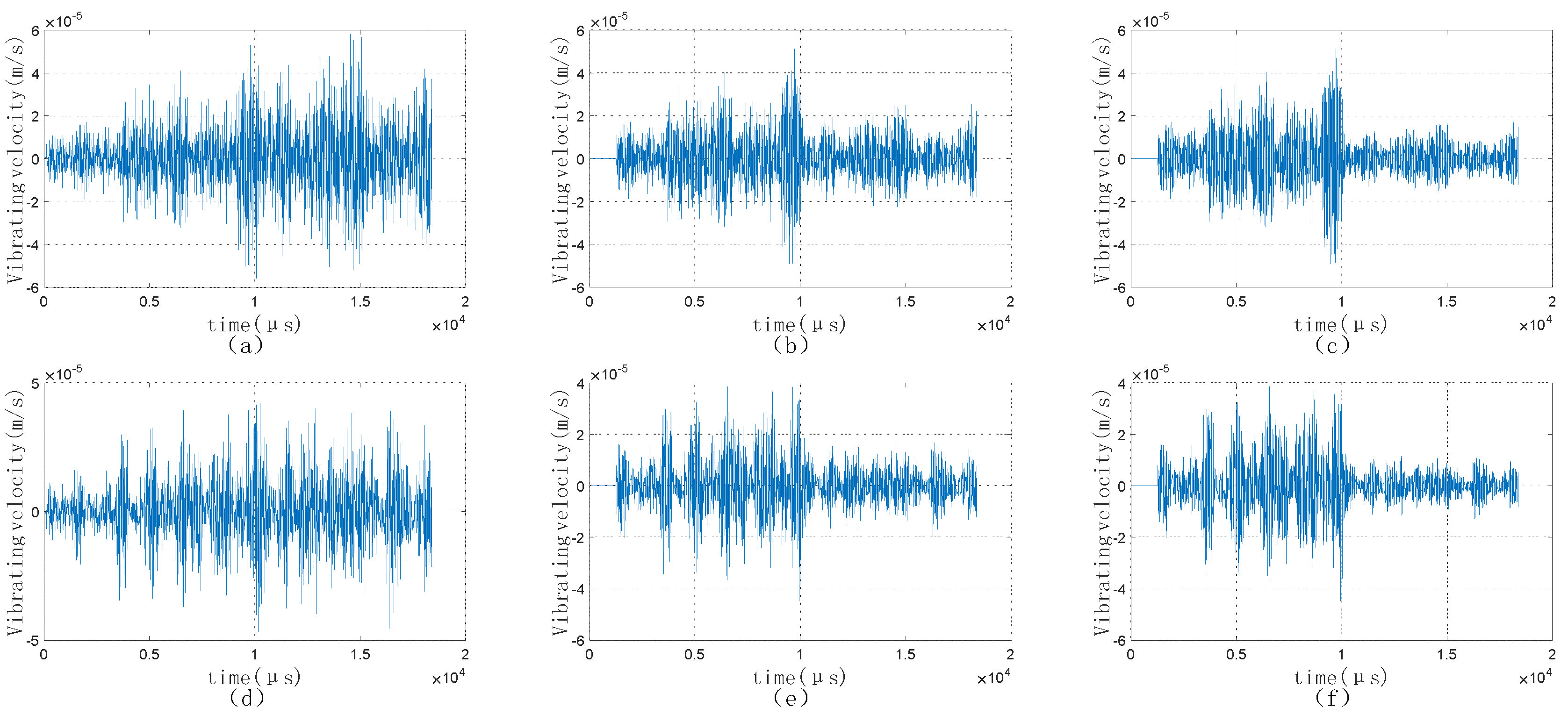
3. Test and Analysis of Compressor Excitation Signal

3.1. Full Band Noise Analysis

In the anechoic chamber, the near-field noise of the compressor under working conditions is tested. Take points at the center line of the main shell and liquid storage tank, respectively, arrange microphones, measure the sound pressure data, and then pass through

$$L_p=20\lg \left(\frac{p}{p_0}\right)$$

(8)

Realize the conversion of sound pressure level, where P₀ = 2 × 10⁻⁵ pa is the reference sound pressure. The location of the measuring points and the near-field sound pressure level of each measuring point are shown in Figure 1 and Figure 2, respectively.

According to Figure 2, the sound pressure level frequency response increases first and then decreases with the frequency. The sound pressure level is large in the range of low intermediate frequency (2000–5000 Hz). After 5000 Hz, the sound pressure level at each measuring point decreases significantly. Compared with the measuring point of the reservoir, the sound pressure level measured at the measuring point of the main shell is higher. In the low and intermediate frequency region, the peak difference of the two sound pressure levels is between 5–10 dB, which is particularly obvious. From the average sound energy density formula [21]:

$$\overline{\epsilon }=\frac{\Delta \overline{E}}{V_0}=\frac{p^2}{2{\rho }_0{c}_0^2}=\frac{p_e^2}{{\rho }_0{c}_0^2}$$

(9)

where p is the sound pressure at the measuring point, p_e = p/√2, is the effective sound pressure, and the sound power is directly proportional to the quadratic power of the sound pressure. Through the conversion of sound pressure and sound pressure level, the sound energy radiated per unit time at the measuring point of the main shell is calculated, which is about 3~9 times that of the corresponding measuring point of the liquid reservoir.

By comparing the noise analysis results, it can be seen that under working conditions, the compressor noise is mainly distributed in the low and medium frequency section, and the sound energy at the main shell is dense. That is, the main shell and its connectors are the main noise source, and the energy distribution of the accumulator shell is sparse and has little impact on the sound radiation of the whole machine. The main characteristics of each excitation source are the shell radiation caused by irregular excitation inside the compressor and the harmonic component of the electromagnetic force with the same modal frequency as the whole machine. Therefore, the active control method for low-frequency vibration and sound signal is used to suppress vibration and sound radiation, and the main frequency band of active control is 1000–5000 Hz. However, it is still necessary to analyze the characteristics of the excitation source and determine the main excitation source.

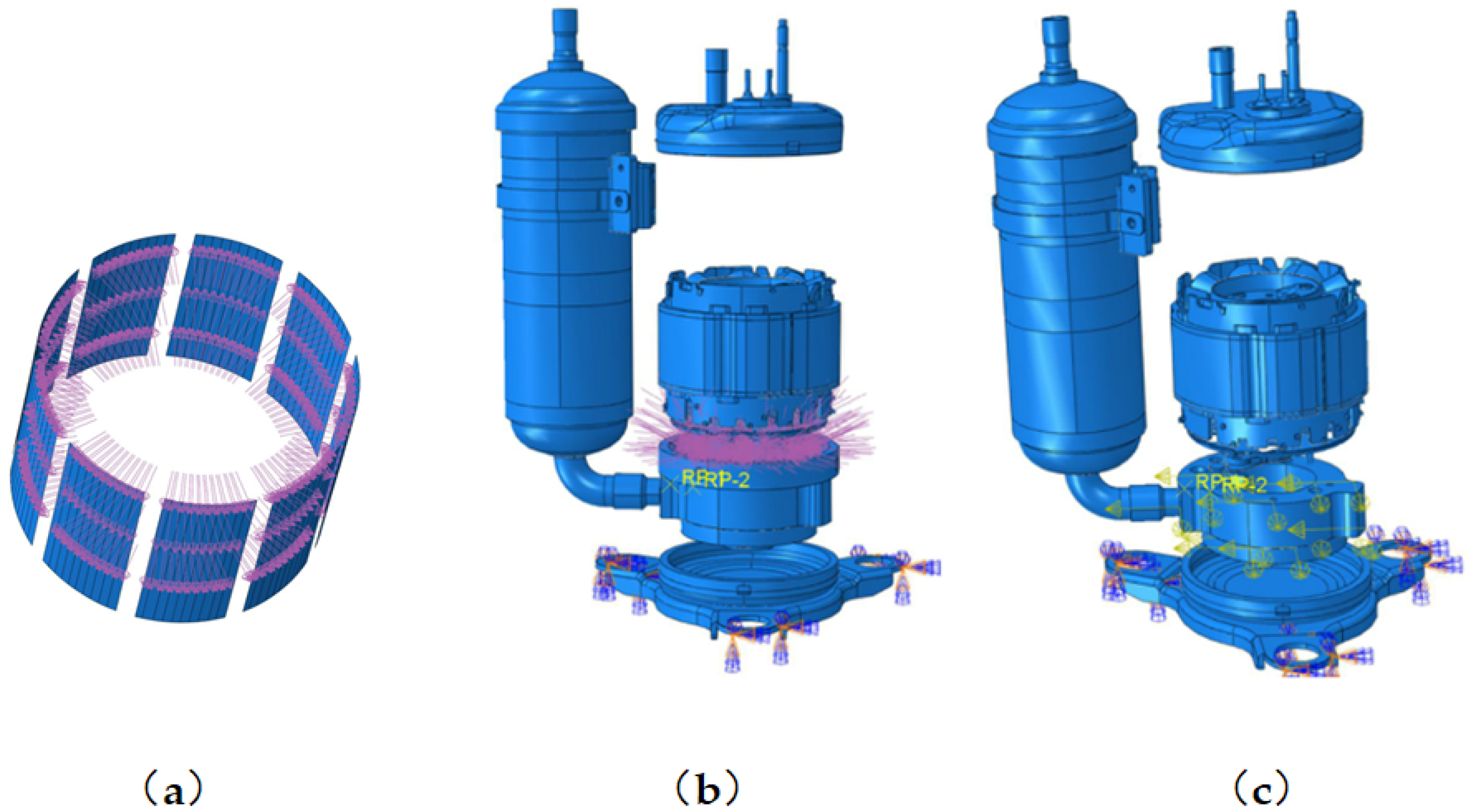
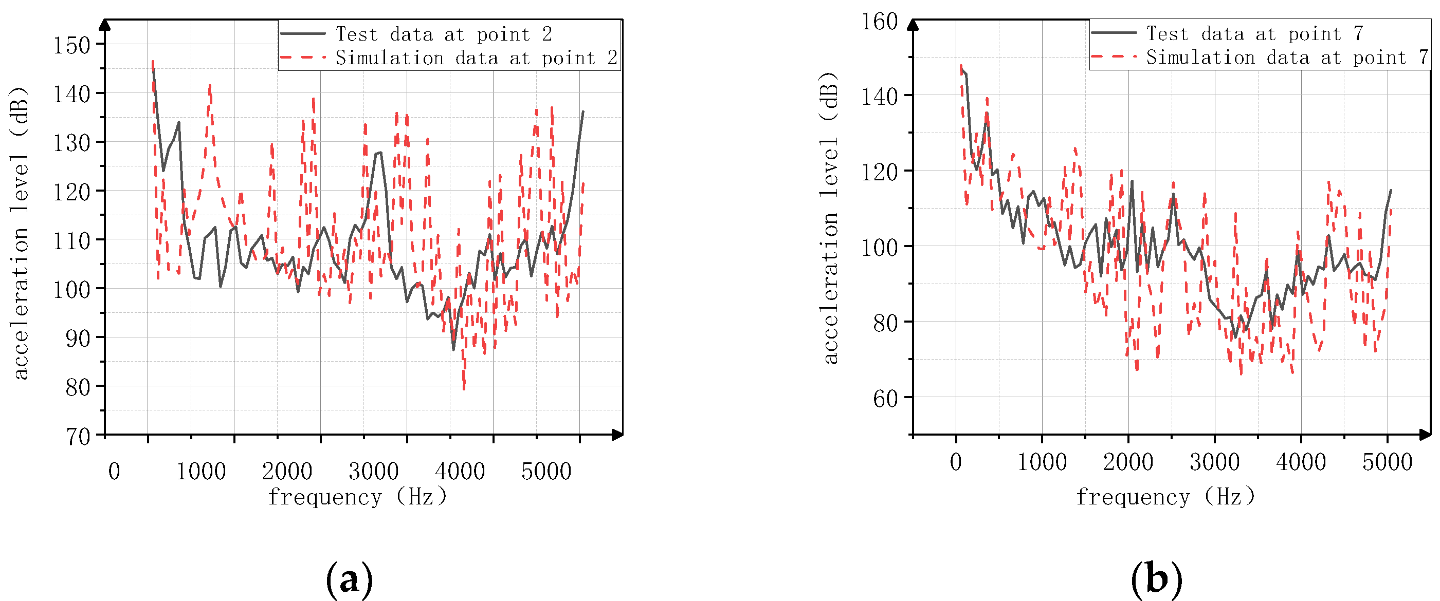
3.2. Simulation Analysis of Excitation Signal

According to the stress analysis of the compressor, the main vibration forces of the compressor are electromagnetic force and aerodynamic force generated by compressed gas, and there are mainly two aerodynamic forces: one is pulsating pressure, and the other is cylinder pressure.

The action mode of electromagnetic noise is generally as follows: electromagnetic force acts on the slot gap between stator and rotor, causing slot air pulsation and stator yoke vibration through tangential and radial electromagnetic force. The coupling relationship between stator and main shell is generally formed through rib connection or interference fit, so as to make the main shell vibrate and radiate noise outward. The main action positions of pulsating pressure include the upper surface of the bearing, the inner and outer surfaces of the outer muffler, the inner and outer surfaces of the inner muffler, the shaft diameter wall in the rotor area, and the shaft diameter wall in the lower cavity. However, its action energy is limited and has little effect on the sound radiation of the shell. For the cylinder pressure, due to the fast speed of the compressor rotor and the short compression cycle, a large pressure will be generated in the compression chamber and the suction chamber inside the cylinder. Finally, the vibration energy will be transmitted to the main shell through the “cylinder bearing main shell” path, resulting in radiated noise.

According to the action relationship of each force on the compressor, the relevant finite element model is established in ABAQUS, and the force at each position is measured by the real machine. According to the measured electromagnetic force data, the magnitude of electromagnetic force is not equal on different pins, and its magnitude is also different at different positions of the same pin. Therefore, each pin is divided into several parts, and each part has a corresponding electromagnetic force data. After converting its time domain data into the frequency domain, it is directly loaded at the corresponding position, as showed in Figure 3a. The figure only shows the loading of the pin and force. For the pulsating pressure, its active position has not changed, so its loading method is also relatively simple. Refer to the extraction of pulsating pressure and apply pulsating pressure at the corresponding position, as showed in Figure 3b. However, the cylinder pressure always changes with the rotation of the crankshaft, which increases the difficulty of loading. Here, firstly, COMSOL software is used to analyze the cylinder separately; the stress amplitude and direction of the whole cylinder at different time are calculated, and then the data is input into ABAQUS to load the cylinder volume force. The loading condition is shown in Figure 3c.

According to the action relationship of the main force, the finite element model of the compressor is loaded, and the acceleration of the compressor shell is simulated and calculated. The arrangement of measuring points is shown in Figure 1. Measuring points 1, 4, 7, and 10 are 50 mm away from the upper surface. Measuring points 3, 6, 9, and 12 are 50 mm away from the lower surface, and measuring points 2, 5, 8, and 11 are 140 mm away from the lower surface. Extract data and draw graphics. It is found that for measuring points 1–6, the acceleration comparison between simulation and test is similar to that of measuring point 2. For test points 7–12, the comparison between simulation and test data is similar to that of test point 7. Therefore, it is only necessary to draw the relationship curve between acceleration level and frequency at measuring point 2 and measuring point 7 to reflect the noise distribution of the compressor. The comparison between simulation and test data is shown in Figure 4.

It can be seen from the above figure that the change trend of simulation and test data is consistent, and there is only a certain gap in amplitude. This is because there are many internal parts of the compressor, and the relationship between different parts is different. In addition to the main excitation source, there are also forces between some small parts. Only the main excitation is considered during loading, and there are some other excitations, such as the knocking of the exhaust valve plate on the baffle and seat ring, the fluid noise caused by the change of channel area in the process of suction and exhaust, etc. Therefore, there are differences in the amplitude between the simulation and test data. However, the change trend is consistent, indicating that the main noise source of the compressor is the excitation source loaded during the simulation, and other noise sources will only affect the noise amplitude in a small range.

4. Improved FULMS Algorithm Active Control

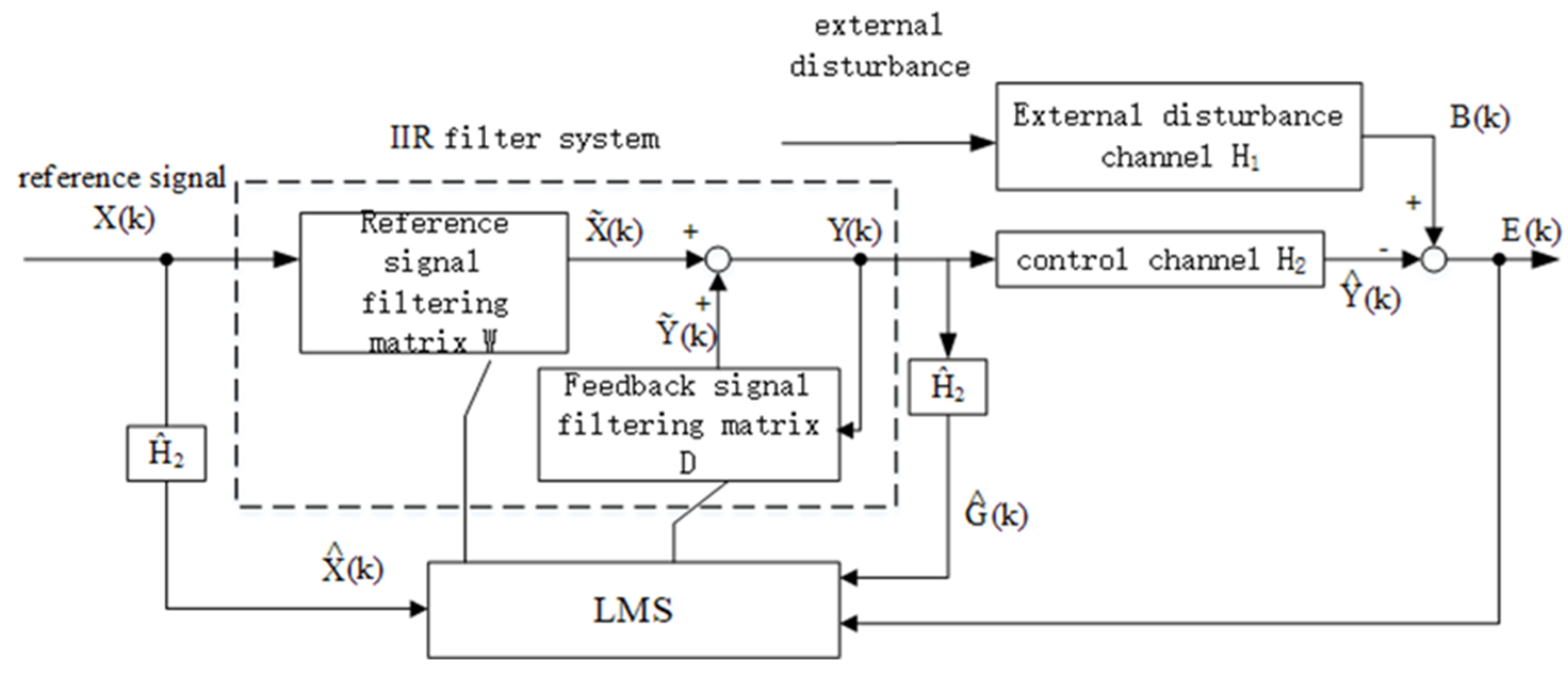
4.1. Improved FULMS Algorithm Based on Nadam

The active control algorithm generally adopts the adaptive filtering algorithm, while the classical algorithms are implemented based on FIR filter. Its transmission function is an all zero structure. In practical application, the feedback of the filtered output signal to the reference signal is not considered. However, this factor should be considered. The FULMS algorithm is a least mean square algorithm composed of IIR filter structure. This feedback has been considered in the actual operation process, which improves the classical algorithm to a certain extent. However, compared with NLMS algorithm, the convergence speed of this algorithm is basically the same. However, due to the acquisition and truncation of the feedback signal, the FUNLMS algorithm has a loss of control efficiency. Therefore, this paper optimizes the FUNLMS algorithm based on the Nadam method.

The structure of the FULMS algorithm is mentioned in many references [22,23], and the specific structure of the FULMS algorithm is shown in Figure 5.

The control system designed in this paper is a multi-channel system, and it includes n controllers and n sensors. The meaning of each signal in the figure is as follows:

(1)

Term B(k) is the n-dimensional response vector generated by the external disturbance signal through the external disturbance channel;

(2)

After the reference signal X(k) with a high degree of correlation with the external disturbance signal is adaptively filtered by the IIR filtering system, an n-dimensional control vector is generated, corresponding to the signal input of n actuators respectively, and then the control signal is generated through the control channel Ŷ(k);

(3)

Term E(k) is the difference between the two signals; when the system has not controlled, there is E(k) = B(k);

(4)

Terms H₁ and H₂ are the transfer functions of the primary channel and the secondary channel, respectively. Term $\hat{\mathrm{H}}$₂ is the modeling matrix of the secondary channel. In an ideal case, $\hat{\mathrm{H}}$₂ = H₂, and they are all n × n-dimensional arrays. Each array has n-dimensional vectors, corresponding to the filter length of each filter.

(5)

Terms $\hat{\mathrm{X}}$(k) and $\hat{\mathrm{G}}$(k)are, respectively, X(k) and Y(k) obtained after the secondary channel simulation, which are the control signals updated by the algorithm.

The FULMS algorithm generally adopts the gradient descent method for iteration, with a general calculation rate, while the classical momentum method [24] (CM) increases the feedback of gradient change to the iteration, reduces the oscillation of iteration during convergence, and speeds up the convergence process. The process can be expressed as follows:

$$\begin{array}{c}{m}_t=\delta m_{t-1}+{\nabla }_t\\ W_{t+1}=W_t-\eta m_t\end{array}\}$$

(10)

where ${\nabla }_t$ represents the gradient at time t, and η is a constant value. At the same time, in order to solve the adaptive problem of gradient in the iterative process, some scholars proposed the gradient adaptive method [25], and its form is as follows:

$$\begin{array}{c}{n}_t=n_{t-1}+{\nabla }_t^2\\ W_{t+1}=W_t-\eta \frac{{\nabla }_t}{\sqrt{n_t}+\epsilon }\end{array}\}$$

(11)

to prevent division error, set a small parameter ε. It has little effect on the calculation results. The algorithm is used in each iteration η. Compared with the L₂ norm of all previous gradients, it can reduce the learning step of significantly changing coefficients and increase the learning step of slightly changing coefficients, so as to stabilize and balance the change level of each coefficient.

Based on the above two gradient optimization algorithms, combined with their advantages and iterative properties, an adaptive momentum gradient descent algorithm (Adam) is proposed. Its structure is as follows [26]:

$$\begin{array}{c}{m}_t=\delta m_{t-1}+\left(1-\delta \right){\nabla }_t\\ {\widehat{m}}_t=\frac{m_t}{1-{\delta }^t}\\ n_t=\nu n_{t-1}+\left(1-\nu \right){\nabla }_t^2\\ {\widehat{n}}_t=\frac{n_t}{1-{\nu }^t}\\ W_{t+1}=W_t-\eta \frac{{\widehat{m}}_t}{\sqrt{{\widehat{n}}_t}+\epsilon }\end{array}\}$$

(12)

where δ, υ are constant values less than one. Aiming at the problems of more fluctuations and slow convergence speed in the convergence process of gradient descent method, Nesterov improved it and proposed Nesterov’s acceleration gradient algorithm (NAG), which is more convenient than gradient descent method and can be rewritten as an improved momentum algorithm. Its form is as follows [27]:

$$\begin{array}{c}{g}_t=df\left(W_t-\eta \delta m_t\right)\\ m_t=\delta m_{t-1}+g_t\\ W_{t+1}=W_t-\eta m_t\end{array}\}$$

(13)

Combining NAG algorithm with Adam, the Nadam algorithm for gradient descent method can be obtained, which can be expressed as [28]:

$$\begin{array}{c}{g}_t=df\left(W_t\right)\\ {\widehat{g}}_t=\frac{g_t}{1-{\delta }^t}\\ m_t=\delta m_{t-1}+\left(1-\delta \right)g_t\\ {\widehat{m}}_t=\frac{m_t}{1-{\delta }^t}\\ n_t=\nu n_{t-1}+\left(1-\nu \right)g_t^2\\ {\widehat{n}}_t=\frac{n_t}{1-{\nu }^t}\\ {\stackrel{-}{m}}_t=\left(1-\delta \right){\widehat{g}}_t+\delta {\widehat{m}}_t\\ W_{t+1}=W_t-\eta \frac{{\stackrel{-}{m}}_t}{\sqrt{{\widehat{n}}_t}+\epsilon }\end{array}\}$$

(14)

Combining the algorithm with FUNLMS can theoretically improve the convergence performance of the algorithm and obtain better control effect. For the FUNLMS algorithm, the gradient can be expressed as the vector product of the error signal and the reference signal through secondary filtering. Nadam optimization is added in the iterative process of filter coefficients. The structure of the control algorithm can be summarized as follows:

$$\begin{array}{ccc}& & \hfill Y_i\left(k\right)=W_i\left(k\right)X_i^T\left(k\right)+D_i\left(k\right)Y_i^T\left(k-1\right))\hfill \\ & & \hfill E_l\left(k\right)=B_l(B)-{\displaystyle \sum _{i=1}^I}{\hat{H}}_{2li}{Y}_i(K)\hfill \\ \hfill g{x}_k=\frac{2{\sum }_{i=1}^L{\hat{H}}_{2li}{X}_i(K)E_l(K)}{1-{\delta }^k}\hfill & ,& \hfill g{y}_k=\frac{2{\sum }_{i=1}^L{\hat{H}}_{2li}{Y}_i(K)E_l(K)}{1-{\delta }^k}\hfill \\ \hfill m{x}_k=\frac{\delta m{x}_{k-1}+\left(1-\delta \right)g{x}_k}{1-{\delta }^k}\hfill & ,& \hfill m{y}_k=\frac{\delta m{y}_{k-1}+\left(1-\delta \right)g{y}_k}{1-{\delta }^k} \hfill \\ \hfill n{x}_k=\frac{vn{x}_{k-1}+\left(1-v\right)g{x}_k^2}{1-v^k}\hfill & ,& \hfill n{y}_k=\frac{vn{y}_{k-1}+\left(1-v\right)g{y}_k^2}{1-v^k}\hfill \\ \hfill \stackrel{-}{m}{x}_k=\left(1-\delta \right)g{x}_k+\delta m{x}_k\hfill & ,& \hfill \stackrel{-}{m}{y}_k=\left(1-\delta \right)g{y}_k+\delta m{y}_k\hfill \\ W\left(k+1\right)=W\left(k\right)-{\mu }_x\frac{\stackrel{-}{m}{x}_k}{\sqrt{n{x}_k}+\epsilon }& ,& \hfill D\left(k+1\right)=D\left(k\right)-{\mu }_y\frac{\stackrel{-}{m}{y}_k}{\sqrt{n{y}_k}+\epsilon })\hfill \end{array}\}$$

(15)

4.2. Secondary Source Configurations

For the improved FULMS algorithm, its basic structure has not changed, and it is still a multi-channel mode, which needs multiple controllers and sensors to control. During the operation of the compressor, there are different modal shapes at different frequencies, and the number and location of secondary sources produces different results.

The number of secondary sources is selected according to certain criteria. Taking the flexible plate as an example, if the damping is ignored, its dynamic equation can be expressed as follows:

$$M_{n\times n}{\ddot{x}}_{n\times 1}+K_{n\times n}{x}_{n\times 1}=L_{n\times r}{u}_{r\times 1}$$

(16)

where M and K are structural mass and stiffness matrices; $\ddot{x}$ and x are acceleration and displacement vector, respectively; u is the input control force; L is the control force vector configuration matrix; n is the degree of freedom of the system; r is the number of actuators. After certain changes and calculations, the eigenvalue equation of energy correlation matrix G can be obtained:

$${\Lambda }_G=\left\{{\lambda }_1,{\lambda }_2,{\lambda }_3,\dots ,{\lambda }_m,0_{m+1},0_{m+2},0_{m+3},\dots ,0_{2m}\right\}$$

(17)

The number of non-zero eigenvalues in the Formula (17) represents the number of modal control forces required in active control, and its amplitude represents the energy generated by the secondary source. Because there are great differences in different eigenvalues in the frequency band that need to be controlled, the larger eigenvalue indicates that the structural vibration is more sensitive, and the required modal energy is larger.

Therefore, only n modes can be selected for control and monitoring by sorting eigenvalues. The modal eigenvalues are sorted from large to small, and the dimensionless ratio is selected δ (generally 90~95%) so that

$$\frac{{\sum }_{i=1}^n{\lambda }_i}{{\sum }_{i=1}^m{\lambda }_i}>\delta$$

(18)

obtains the minimum n value satisfying the Formula (18) and obtains the energy contribution to the system under the same excitation δ, the minimum number of modal forces, in other words, the minimum number of modes to be controlled. However, for the compressor housing, the value of λ_i is difficult to obtain in analytical form. Since the eigenvalue can represent the modal energy, it is transformed into the vibration energy of the compressor shell at each modal frequency. Therefore, the number of secondary sources shall meet the following formula:

$$\frac{{\sum }_{i=1}^n{E}_i}{{\sum }_{i=1}^m{E}_i}>\delta$$

(19)

in the Formula (19), E_i represents the total energy of the i-th mode and the sum of modal kinetic energy and modal strain energy.

Based on the previous modal analysis results, 20 Pa white noise is applied from the lower boundary of the stator to the lower boundary of the cylinder, and the modal energy data corresponding to all characteristic frequencies in the frequency band to be controlled are calculated, as shown in

Table 1. Energy proportion of each mode.

Characteristic Frequency	Corresponding Energy	Energy Proportion
3672	1.71 × 10−6	77.1171%
3469	5.06 × 10−7	22.8296%
1231	8.48 × 10−10	0.0383%
2884	1.58 × 10−10	0.0071%
3660	1.03 × 10−10	0.0046%
2885	5.98 × 10−11	0.0027%
1741	5.66 × 10−12	0.0003%
3376	2.86 × 10−12	0.0001%
3966	2.30 × 10−12	0.0001%
1242	9.76 × 10−13	0.0000%
1760	1.77 × 10−13	0.0000%

below.

It can be seen from the table that the energy is mainly concentrated at 3672 Hz and 3469 Hz. These two frequencies correspond to the ninth and seventh modes of the compressor shell, respectively. Therefore, it is mainly necessary to control these two modes during noise reduction. According to the COMSOL simulation results, the modal vibration modes are shown in Figure 6.

According to the modal shapes, it can be seen that the compressor shell has 4 and 6 peak areas, respectively, under these two modes. Therefore, in order to effectively control these two order vibration modes, six secondary sources are selected.

The location configuration of secondary sources needs to consider two problems: configuration criteria and optimization algorithm. In this paper, the controllability/observability criterion is mainly used to determine the actuator/sensor position. The optimization algorithm adopts the particle swarm optimization algorithm and uses the joint simulation of COMSOL and MATLAB to optimize the position configuration scheme and find the best secondary source position, so as to realize the active vibration control of the compressor main shell under the condition of optimal observability/controllability. The sensor position and vibration mode to be controlled are as follows:

The blue circle in the figure refers to the position of the active controller. According to the above figure, the position of the control point is basically located at the peak of the vibration mode, which has a strong correlation with the modal vibration mode, and the active vibration control based on the vibration mode can be realized. The generalized coordinates of each point are shown in

Table 2. Actuator/sensor position coordinates.

Point Serial Number	X (m)	Y (m)	Z (m)
1	0.0453	0.0650	0.0121
2	0.0118	0.0648	0.0453
3	−0.0461	0.0809	0.0086
4	−0.0447	0.0735	−0.0142
5	0.0036	0.0621	−0.0467
6	0.0455	0.1075	−0.0111

.

Therefore, using particle swarm optimization algorithm and joint simulation, the point combination with the strongest effect on vibration suppression and monitoring of the main shell is determined, the actuator/sensor position is configured, and 6 × 6 multi channel control model is used for the research of active vibration control of the research object.

4.3. Joint Simulation Analyses

Due to the irregular structure of the compressor, the current research on its vibration and sound radiation is insufficient, and the experimental conditions are incomplete, so it is difficult to simulate the real operating conditions. Therefore, this paper mainly adopts the joint simulation form, combined with finite element analysis and algorithm control to simulate the data exchange and excitation loading process in the actual test, effecting verification and control capability analysis of active control algorithm at low cost.

In the simulation of the active control effect, using programming software carries out data exchange and iterative calculation of control force amplitude and filter coefficient. Using software for finite element analysis, the control force amplitude is updated each time, finite element analysis of the mechanical field is carried out, and the vibration response of the corresponding measuring points is obtained each time. With the iteration, the data are continuously exchanged between the two to realize the simulation of the active control algorithm.

The data exchange process and iterative steps in actual operation are shown in Figure 7.

In Figure 8, the blue dotted line box indicates the model processing in software of finite element analysis, and the red solid line box indicates the iterative operation of data in programming software.

According to the above simulation methods, active control effects of the Nadam-FUNLMS and FUNLMS algorithms are simulated and compared. White noise excitation is defined in the corresponding shell section from the lower boundary of stator to the lower boundary of cylinder to simulate the irregular disturbance caused by fluid pulsation under working conditions and fix the lower boundary of main shell δ = 0.99, υ = 0.999, β = ε = 10⁻⁸, α = 0.0015; the total time step for analysis is 0~220,000 μs.

After the structure is excited for 0.2 s, add a secondary force source to perform active control, conduct simulation, obtain the time-domain response of vibration velocity at each measuring point under the control of Nadam-FUNLMS algorithm, and compare the corresponding data of FUNLMS algorithm and uncontrolled system. The vibration velocity of some measuring points can be obtained, as showed in Figure 9.

The following can be seen in Figure 9:

(1) After adding the FUNLMS algorithm control, the surface vibration velocity of measuring point 1 and measuring point 3 decreased significantly, and with the passage of time, the effect of active control became more and more obvious. When the time reaches 10,000 μs, the control effect is stable, and the peak vibration speed is reduced by more than half, which effectively reduces the vibration energy of the node.

(2) After the FUNLMS algorithm is optimized by Nadam, the convergence speed of the algorithm is accelerated; the peak vibration speed of measurement points 1 and 3 is further reduced, and the convergence speed and control effect are better than those of the unoptimized algorithm.

After the surface vibration velocity of the main shell is squared, the surface integral is taken. This value is positively correlated with the total kinetic energy of the structure, which can be used to evaluate the overall control of the structure by various algorithms. After 10,000 μs of control is added, the system response to steady state is evaluated, and the curve is smoothed. Results of the Nadam-FUNLMS, FUNLMS, and no control system are shown in Figure 9.

As can be seen in Figure 10:

(1) By suppressing the response of the selected optimal control point, the overall vibration response of the main casing is weakened, thereby reducing the sound radiation level of the structure and reducing the noise of the compressor.

(2) With the increase of action time, the kinetic energy suppression effect of the active control process on the system is gradually obvious and tends to be stable. After the active control is added, the steady-state response of the system will be reduced by 3~6 dB.

(3) The suppression of structural vibration by the Nadam-FUNLMS and FUNLMS algorithms is similar. Among them, the suppression effect of Nadam-FUNLMS on system kinetic energy is slightly better than that of the FUNLMS algorithm.

The numerical simulation shows that the Nadam-FUNLMS algorithm has a better convergence speed in the process of active control and can effectively realize vibration suppression in a short time to meet the rapidity requirements of its active control algorithm in the actual use situation.

5. Conclusions

Starting from the structure–sound radiation modal relationship, this paper studies the multi-modal active control of the compressor shell, designs a scheme, and tests the effect of the active control. The specific conclusions are as follows:

(1) The relationship between the vibration mode and the sound radiation mode is determined by theoretical calculation, and it is confirmed that the sound radiation can be controlled by controlling the vibration mode.

(2) Through the simulation analysis of the compressor excitation signal, the acceleration of the compressor shell is obtained. Compared with the experiment, it is determined that the main noise sources are electromagnetic force, pulsating pressure, and cylinder fluid pulsating pressure.

(3) Based on the Nadam and step normalization method, the multi-mode active vibration control FULMS algorithm is improved to improve its convergence. According to the modal energy distribution of the compressor shell, it is determined that the modal orders to be controlled in multi-mode active control are the 7th and 9th orders.

(4) The particle swarm optimization algorithm is used to determine the point combination with the strongest effect on vibration suppression and monitoring of the main shell and establish a 6 × 6 multi channel control model. Based on this, an active control simulation scheme is proposed, which is used to simulate the effect of active control and evaluate the performance of each algorithm. The improved FULMS algorithm converges faster and has better effect.

References

1. Ooi, K.; Wong, T. A computer simulation of a rotary compressor for household refrigerators. Appl. Therm. Eng. 1997, 17, 65–78. [Google Scholar] [CrossRef]
2. Ooi, K. Design optimization of a rolling piston compressor for refrigerators. Appl. Therm. Eng. 2005, 25, 813–829. [Google Scholar] [CrossRef]
3. Ferraris, G.; Andrianoely, M.A.; Berlioz, A.; Dufour, R. Influence of cylinder pressure on the balancing of a rotary compressor. J. Sound Vib. 2006, 292, 899–910. [Google Scholar] [CrossRef]
4. Kim, H.J. Transmission Loss and Back Pressure Characteristics for Compressor Mufflers. In Proceedings of the 1992 International Compressor Engineering Conference at Purdue, Purdue University, West Lafayette, IN, USA, 14–17 July 1992; pp. 1455–1462. [Google Scholar]
5. Dreiman, N.; Herrick, K. Vibration and control of a rotary compressor. In Proceedings of the 1998 International Compressor Engineering Conference at Purdue University, West Lafayette, IN, USA, 14–17 July 1998; pp. 685–690. [Google Scholar]
6. Widrow, B. A Review of Adaptive Antennas. In Proceedings of the IEEE International Conference on Acoustics, Washington, DC, USA, 2–4 April 1979; pp. 273–278. [Google Scholar]
7. Morgan, D. An analysis of multiple correlation cancellation loops with a filter in the auxiliary path. IEEE Trans. Acoust. Speech Signal Process. 1980, 28, 454–467. [Google Scholar] [CrossRef]
8. Burgess, J.C. Active adaptive sound control in a duct: A computer simulation. J. Acoust. Soc. Am. 1981, 70, 715–726. [Google Scholar] [CrossRef]
9. Saito, N.; Sone, T. Influence of modeling error on noise reduction performance of active noise control systems using filtered-X LMS algorithm. J. Acoust. Soc. Jpn. (E) 1996, 17, 195–202. [Google Scholar] [CrossRef] [Green Version]
10. Douglas, S. Fast implementations of the filtered-X LMS and LMS algorithms for multichannel active noise control. IEEE Trans. Speech Audio Process. 1999, 7, 454–465. [Google Scholar] [CrossRef] [Green Version]
11. Das, D.; Kuo, S.; Panda, G. New block filtered-X LMS algorithms for active noise control systems. IET Signal Process. 2007, 1, 73–81. [Google Scholar] [CrossRef]
12. Eriksson, L.J. The development of the filtered-U algorithm for active noise control. J. Acoust. Soc. Am. 1991, 89, 257–262. [Google Scholar] [CrossRef]
13. Kim, I.; Na, H. Constraint filtered-x and filtered-u least-mean-square algorithms for the active control of noise in ducts. J. Acoust. Soc. Am. 1994, 95, 3379–3389. [Google Scholar] [CrossRef]
14. Suman, T.; Venkatanarayana, M. Active Noise Control for PVC Duct Using Robust Feedback Neutralization F×LMS Approach. J. Control. Autom. Electr. Syst. 2021, 32, 1189–1203. [Google Scholar] [CrossRef]
15. Ospel, M.W.; Werner, P.; Wurm, F.H.; Witte, M. Simulation of active noise control using transform domain adaptive filter algorithms linked with the inhomogeneous Helmholtz equation. Appl. Acoust. 2021, 182, 108250. [Google Scholar] [CrossRef]
16. Ramos, L.P.; Martín, F.R.; Arranz, M.F.; Palacios, -N.G. An Alternative Approach to Obtain a New Gain in Step-Size of LMS Filters Dealing with Periodic Signals. Appl. Sci. 2021, 11, 5618. [Google Scholar] [CrossRef]
17. Gaiotto, S.; Laudani, A.; Lozito, G.M.; Riganti, F.F. A Computationally Efficient Algorithm for Feedforward Active Noise Control Systems. Electronics 2020, 9, 1504. [Google Scholar] [CrossRef]
18. Mondal, K.; Das, S.; Hamada, N.; Abu, A.B.; Das, S.; Faris, W.F.; Toh, H.T. Ahmad, A. An improved narrowband active noise control system without secondary path modelling based on the time domain. Int, J. Veh, Noise Vib. 2019, 15, 110–132. [Google Scholar] [CrossRef]
19. Elliott, S.J.; Johnson, M.E. Radiation modes and the active control of sound power. J. Acoust. Soc. Am. 1993, 94, 2194–2204. [Google Scholar] [CrossRef]
20. Currey, M.N.; Cunefare, K.A. The radiation modes of baffled finite plates. J. Acoust. Soc. Am. 1994, 98, 1570–1580. [Google Scholar] [CrossRef]
21. Blake, W.K. Mechanics of Flow-Induced Sound and Vibration; Inc. (London) Ltd.: London, UK; Academic Press: Cambridge, MA, USA, 1986. [Google Scholar]
22. Xie, L.; Qiu, Z.-C.; Zhang, X.-M. Vibration control of a flexible clamped-clamped plate based on an improved FULMS algorithm and laser displacement measurement. Mech. Syst. Signal Process. 2016, 75, 209–227. [Google Scholar] [CrossRef]
23. Huang, Q.; Luo, J.; Li, H.; Wang, X. Analysis and implementation of a structural vibration control algorithm based on an IIR adaptive filter. Smart Mater. Struct. 2013, 22, 85008. [Google Scholar] [CrossRef]
24. Polyak, B. Some methods of speeding up the convergence of iteration methods. USSR Comput. Math. Math. Phys. 1964, 4, 1–17. [Google Scholar] [CrossRef]
25. Duchi, J.; Hazan, E.; Singer, Y. Adaptive Subgradient Methods for Online Learning and Stochastic Optimization. In Proceedings of the COLT 2010—The 23rd Conference on Learning Theory, Haifa, Israel, 27–29 June 2010. [Google Scholar]
26. Kingma, D.; Ba, J. Adam: A Method for Stochastic Optimization. arXiv 2004, arXiv:1412.6980. Available online: https://arxiv.org/pdf/1412.6980.pdf (accessed on 16 February 2022).
27. Nesterov, Y.E. A method of solving a convex programming problem with convergence rate O (1/k2). Soviet Math. Doklady. 1983, 27, 372–376. [Google Scholar]
28. Dozat, T. Incorporating Nesterov Momentum into Adam. Workshop Track—ICLR 2016. Available online: https://openreview.net/forum?id=OM0jvwB8jIp57ZJjtNEZ (accessed on 16 February 2022).
Figure 1. Microphone arrangement. The numbers 1-12 indicate the positions of the 12 survey points. Measuring points 1, 4, 7, and 10 are 50 mm away from the upper surface. Measuring points 3, 6, 9, and 12 are 50 mm away from the lower surface, and measuring points 2, 5, 8, and 11 are 140 mm away from the lower surface.
Applsci 12 03941 g001
Figure 2. Sound pressure level frequency response of each measuring point: (a) measuring point of the main shell; (b) measuring point of the reservoir.
Applsci 12 03941 g002
Figure 3. Force loading position (a) electromagnetic force; (b) pulsating pressure; (c) cylinder pressure.
Applsci 12 03941 g003
Figure 4. Relationship between acceleration level and frequency (a) measuring point 2; (b) measuring point 7.
Applsci 12 03941 g004
Figure 5. The structure of the FULMS algorithm, LMS—The Least Mean Squares.
Applsci 12 03941 g005
Figure 6. Modal diagram: (a) 3469 Hz, (b) 3672 Hz.
Applsci 12 03941 g006
Figure 7. Correspondence between selecting point of secondary source and modal shape: (a) 3469 Hz, (b) 3672 Hz.
Applsci 12 03941 g007
Figure 8. Data exchange in joint simulation.
Applsci 12 03941 g008
Figure 9. Variation of vibration velocity at some sensor positions: (a) no control of measuring point 1; (b) FUNLMS control of measuring point 1; (c) Nadam-FUNLMS control of measuring point 1; (d) no control of measuring point 3; (e) FUNLMS control of measuring point 3; (f) Nadam-FUNLMS control of measuring point 3.
Applsci 12 03941 g009
Figure 10. Comparison of overall structural response.
Applsci 12 03941 g010