Abstract
Deep convolutional neural networks with strong expressive ability have achieved impressive performances in single-image super-resolution algorithms. However, excessive convolutions usually consume high computational cost, which limits the application of super-resolution technology in low computing power devices. Besides, super-resolution of arbitrary scale factor has been ignored for a long time. Most previous researchers have trained a specific network model separately for each factor, and taken the super-resolution of several integer scale factors into consideration. In this paper, we put forward a multi-scale factor network (MFN), which dynamically predicts the weights of the upscale filter by taking the scale factor as input, and generates HR images with corresponding scale factors from the weights. This method is suitable for arbitrary scale factors (integer or non-integer). In addition, we use an information distillation structure to gradually extract multi-scale spatial features. Extensive experiments suggest that the proposed method performs favorably against the state-of-the-art SR algorithms in term of visual quality, PSNR/SSIM evaluation indicators, and model parameters.
1. Introduction
In computer vision, single image super-resolution (SISR) is currently a hot research topic, which reconstructs a high-resolution (HR) image from a low-resolution (LR) image through image processing methods in the same scene [1]. SISR is widely used in the fields of medicine, transportation, and remote sensing. Since one LR image can generate several HR images, SISR has no unique solution [2]. To address this problem, numerous image SR methods based on deep neural network architectures have been proposed and have shown prominent performance.
Since deep learning shows strong advantages in various computer vision tasks, Dong et al. [3,4] achieved feature extraction, nonlinear matching, and image reconstruction by a three-layer network. VDSR [5] expanded dramatically the depth of the network to 20 by stacking multiple layers to enhance the receptive field. At the same time, Kim et al. [6] proposed DRCN for the first time to apply recursive learning to SR tasks. Tai et al. [7] first adopted a DRRN to reduce parameters. In addition, Tai et al. [8] used a persistent memory network (Mem-Net) that stacks with a densely connected structure to resolve the dependency problem. EDSR [9] removed the batch normalization (BN) layer and used the residual scaling to speed up the training. Zhang et al. [10] added densely connected blocks to the residual to form a residual dense network (RDN). The RDN makes full use of global and local features to enhance SR performance. GFSR [11] used a gradient-guided and multi-scale feature network for image super-resolution. HRFFN [12] designed an enhanced residual block (ERB) containing multiple mixed-attention blocks (MABs) to boost the representative ability of the network. The above algorithms all increased the network depth to upgrade the quality of images [13]. Kim Seonjae proposed two lightweight neural networks with a hybrid residual and dense connection structure to improve the super-resolution performance [14]. However, they usually ignore the problems such as memory consumption and the network is prone to overfitting.
As for the upsampling methods, most use post-upsampling, and need to train a single model for each magnification. Dong et al. first upscaled the resolution as the output size in SRCNN [3,4]. Then they proposed FSRCNN [15], which used a transposed convolution at the end of the network to finish the upsampling operation. Afterwards, Lai et al. [16,17] believed that when the scale factor is large (×8), it is difficult to restore image texture through a one-step operation. So, they proposed Lap-SRN [16,17], which progressively extracted image features and achieved image super-resolution. Shi et al. [18] first used the sub-pixel convolution to upscale the size of feature map for reducing computation. In recent years, many methods have used sub-pixel convolution, such as EDSR [1] and RCAN [19]. However, these SISR methods only consider certain integer scale factors (×2, ×4, ×8). We need to train a module for each scale factor. LESRCNN [20] can obtain a high-quality image by a model for different scales. Few previous works have discussed how to implement super-resolution of the arbitrary scale factor. Meta-SR [21] first proposed to use a single model to achieve multiple magnification.
To solve the above problems, we propose a multi-factor image super-resolution network based on information distillation (IDMF-SR) to realize arbitrary scale SR with the smallest parameters. IDMF-SR mainly includes two parts: a feature learning block and a multi-scale factor upsampling block. The feature learning block is a collection of several information distillation modules. In the information distillation structure, four 3 × 3 convolutions are used to extract image features. After each convolutional layer, a channel split operation divides the extracted features into two parts, and one part is sent to the next convolutional layer, while another part of the feature is retained. We adopted a channel attention mechanism based on contrast-aware. Then the retained feature maps are fused through concatenation at the end. The feature fusion is carried out according to the importance of the feature maps. In the upsampling steps, we adopted a multi-factor network, which includes position projection, weight prediction, and feature mapping. As shown in Figure 1, our IDMF-SR achieves better visual results compared with state-of-the-art methods.
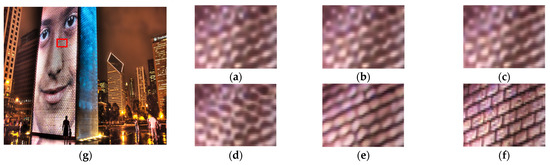
Figure 1.
Visual results under ×4 upscale factor. (a) VDSR; (b) Lap-SRN; (c) Meta-SR; (d) RCAN; (e) IDMF-SR; (f) HR; (g) Urban100 img_76 (3×).
The contribution of this paper can be summarized as the following four points:
- We propose the multi-scale factor image super-resolution network (IDMF-SR) based on information distillation for significantly reducing the number of parameters. Our IDMF-SR is an end-to-end network model, which can utilize hierarchical features more than previous CNN-based methods and balance performance against applicability;
- We put forward a new information distillation network to gradually extract and cascade features. IDN divides the feature map extracted from each layer into two parts. One of the parts flows into the next convolutional layer, and the retrained part is cascaded in the end;
- We propose a contrast-aware channel attention mechanism (CCAM) in the information distillation network. The traditional channel attention mechanism obtains the importance of the channel through the squeeze-and-excitation module, which is conducive to improving the PSNR value. Our CCAM can further enhance image details, such as edges, textures, and structures;
- IDMF-SR is inspired by meta-learning, and the network achieves image magnification by predicting filter weights by scale factors. Only training one network model can realize the image magnification at any multiple, which is conducive to application in the real scene.
2. Materials and Methods
2.1. Network Structure
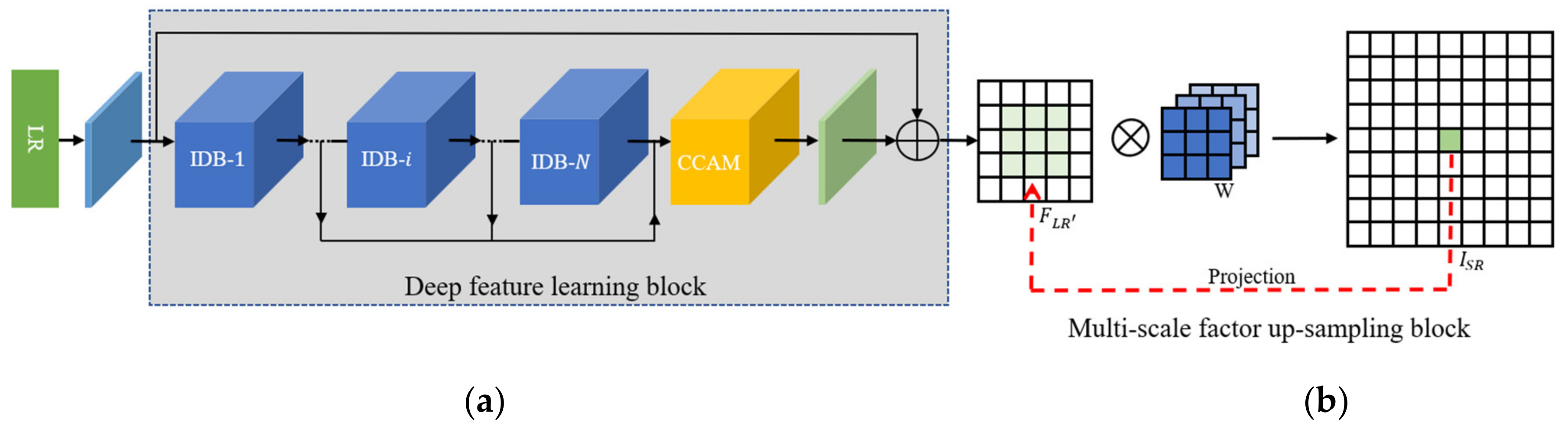
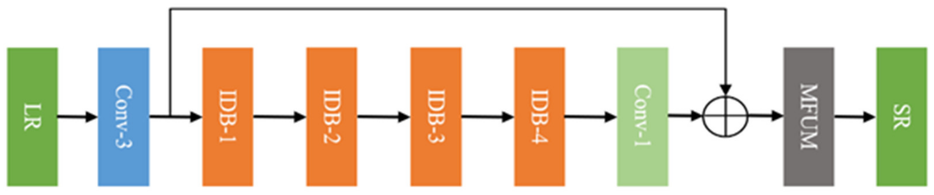
IDMF-SR mainly includes two parts: a deep feature learning block and a multi-scale factor up-sampling block, as shown in Figure 2. First, a Conv-3 is used to extract coarse image features. The key component of IDMF-SR utilizes multiple-stacked information distillation blocks (IDBs). After each information distillation block, the feature maps flow into the next IDB and flows on to the last IDB. When several convolution operations are completed, the retained multi-scale feature maps are fused through concatenation. The upsampling module mainly includes position projection, weight prediction, and feature mapping, as shown in Figure 2. Details are introduced in Section 2.3.
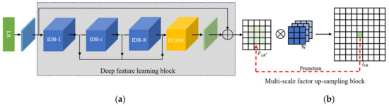
Figure 2.
Network architecture of multi-factor image super-resolution based on information dis-tillation (IDMF-SR). (a) The blue box represents Conv-3; (b) The green box represents Conv-1.
2.2. Information Distillation Module
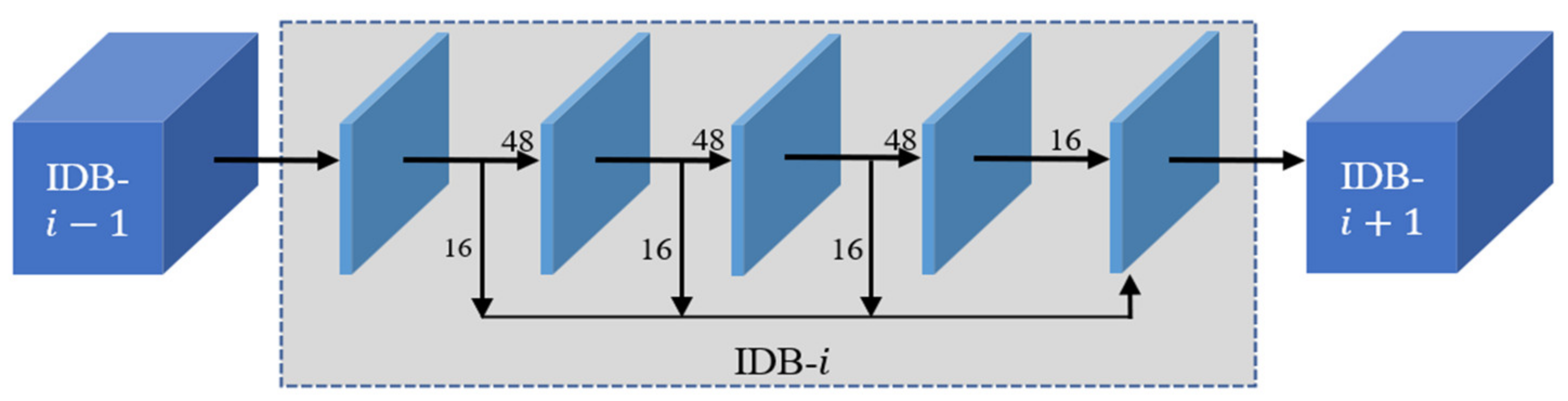
In Figure 3, the information distillation block firstly uses four 3 × 3 convolutions to progressively extract image features. After each convolution, a channel split operation is used to divide the feature maps into two parts. One of the parts flows into the next convolutional layer, and the other part is retained. Finally, the retained feature maps are concatenated to flow into the next IDB. Assuming that the input of the information distillation module is , the process can be expressed as Formulas (1)–(4).

Figure 3.
Information distillation module.
represents the first convolutional layer of the information distillation module, , , , and so on. represents the first channel split layer of the information distillation module. represents the first retained feature maps, and represents the first coarse feature, which is fed into the next calculation unit. After each level of convolutional layer, the feature maps are divided into two parts. Two-thirds flow into the next level, and one-third are retained. Table 1 shows the hyperparameter in the information distillation module. We set 3 × 3 as the kernel size in the convolutional layer. The output channels numbered 64, 48, and 16 are the convolutional layer. The number of the retained feature maps are 16, after four convolutional layers, the number of the output channels is also 64. The convolution kernel and stride follow the common operations in the SISR method.

Table 1.
Convolutional parameter setting in the information distillation module.
Next, we connect the previously retained feature maps , which can be expressed by Formula (5):
We discard the traditional channel attention mechanism and add contrast variables to the original channel attention. In low-level image tasks, such as image super-resolution reconstruction, the contrast-based channel attention mechanism can enhance image details, such as edges and textures. In Figure 4, the contrast is the sum of the standard deviation and the mean. Assuming that the input feature has C feature maps, the size of each feature map is H × W, and the input is expressed as , and the contrast is calculated as Formula (6):
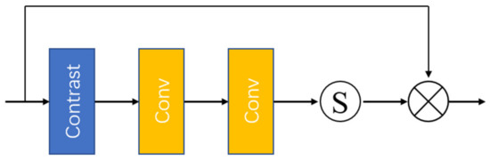
Figure 4.
Contrast-based channel attention mechanism (S is sigmoid function).
Among them, represents the global contrast information measurement function of the feature map, represents the standard deviation, and represents the mean. IDMF-SR can effectively enhance image texture and improve SISR performance by using the contrast-based channel attention mechanism.
2.3. Multi-Factor Upsampling Module
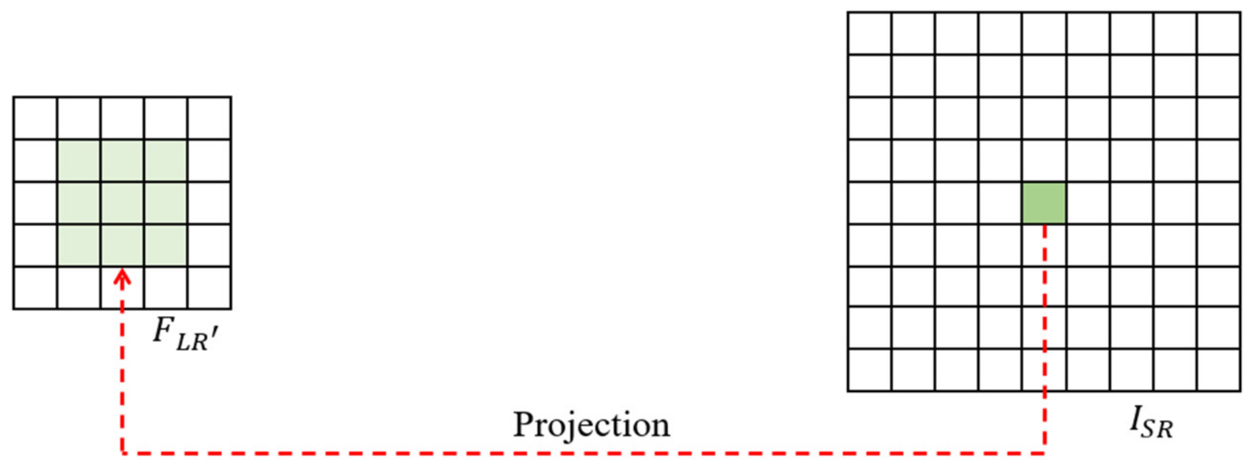
The upsampling module mainly includes position projection, weight prediction, and feature mapping. The Location Projection projects pixels onto the LR image. The Weight Prediction Module predicts the weights of the filter for each pixel on the SR image. Finally, the Feature Mapping function maps the feature on the LR image with the predicted weights back to the SR image to calculate the value of the pixel. After extracts image features through the information distillation module, the output feature map is , and the network finally outputs . According to the principle that a pixel on the HR image can be back-projected to the , pixel on the can be determined by a pixel on the LR image and the filter weight. Therefore, the upsampling module needs a specific filter to match and . The formula is shown in Formula (7). is the mapping function from to . represents the pixel on the , and represents the pixel on the .
- (1)
- Position projection
Position projection is to back-project onto , as shown in Figure 5. The value of pixel on is determined by the point on .the relationship between these two pixels is expressed by Formula (8).
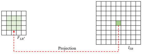
Figure 5.
Location projection schematic diagram.
Among them, is the conversion function, which converts the point into . is floor function, and is scale-factor. It can be seen that adding a scale factor to calculate the relationship between two pixels is suitable for SISR with any scale factor.
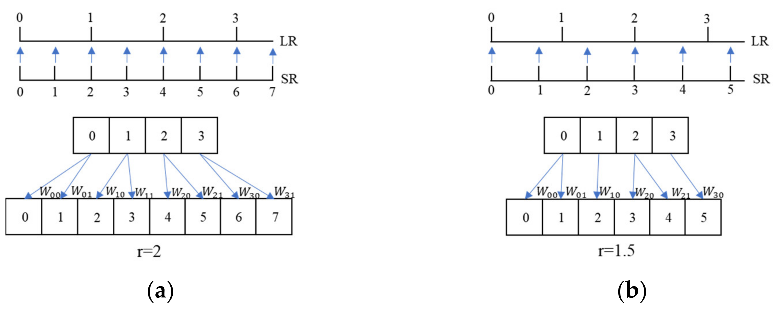
The Location Projection can upscale the feature maps with arbitrary scale factor. The scale factor is divided into two types: integer and non-integer. When is an integer, for example, when is 2, one pixel in the LR image can determine two pixels in the HR image, as shown in Figure 6a. When the scale factor is a non-integer, for example, is 1.5, one pixel in the LR image determines one or two pixels in the HR image, as shown in Figure 6b. No matter whether is an integer or a non-integer, there is always a unique point on the LR image corresponding to a point on the SR image, and these two pixels are called the most relevant pixel pair.
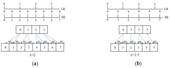
Figure 6.
Pixel mapping schematic diagram. (a) r = 2; (b) r = 1.5.
Different from the typical upscale module, we use a network to predict the filter weights. This process is called weight prediction, expressed by Formula (9):
represents the weight prediction process, is the input of the weight prediction network, is the parameter of the weight prediction network, and is the weight at the pixel . At the pixel , the input of can be expanded to the relative offset of , which is expressed as followed by Formula (10):
To train multiple scale factors for a network, we add scale factor to the expression of . Assuming that the image is upscaled by 2 and 4, then and are obtained. Arbitrary pixels on will have the same filter weights and position projection coordinates as pixels on . Therefore, we improve the expression to the Formula (11):
The weight prediction network is the key of IDMF-SR. Its input is the vector related to the pixel , and the weight matrix is generated through several fully connected layers and activation layers, as shown in Figure 7. Finally, the size of the weight matrix is , represents the number of , represents the number of channels of the predicted HR image, and is the size of kernel.

Figure 7.
Weight prediction network schematic diagram.
- (2)
- Feature mapping
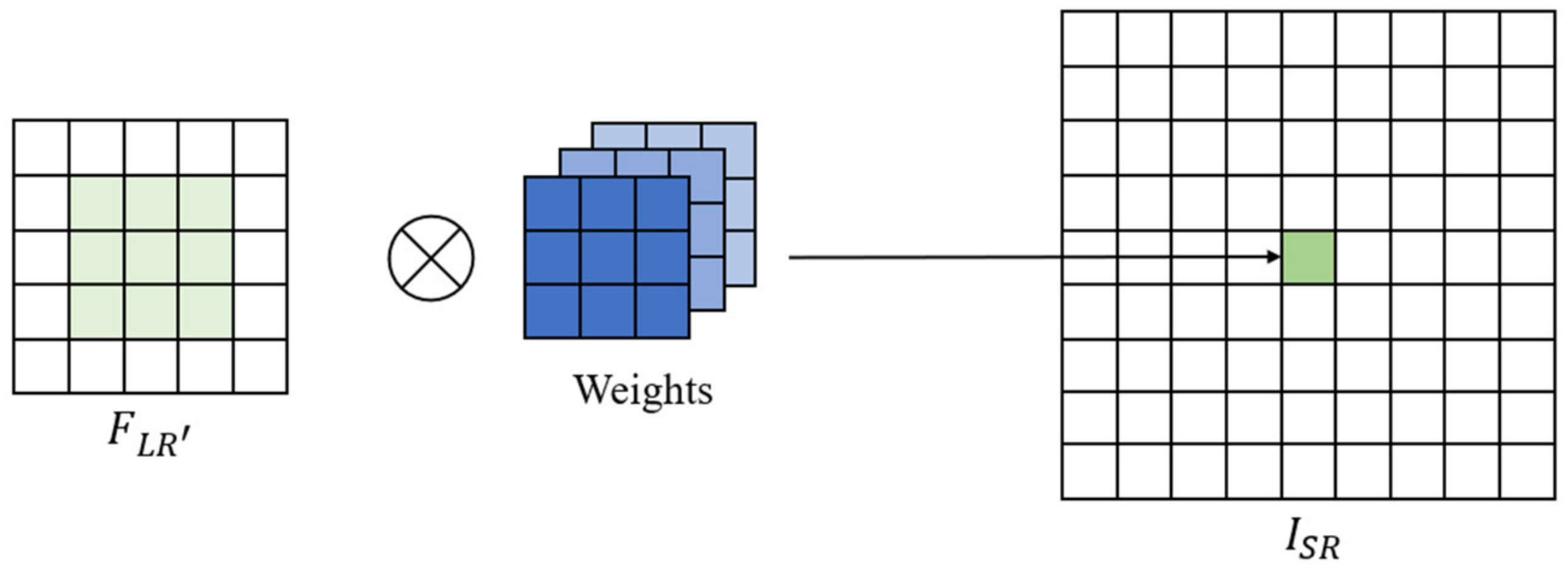
We got the feature of on the LR image from . We predict the filter weights with weight prediction network. The last step is feature mapping, that is, is mapped onto the SR image, as shown in Figure 8. We multiply and the weights to get , as expressed in Formula (12):

Figure 8.
Feature mapping schematic diagram.
2.4. Datasets and Evaluation Metrics
In our experiments, we train the network by DIV2K [22], which contains 800 high-quality images. We use Set5 [23], Set14 [24], BSD100 [25], and Manga109 [26] for evaluation. There are two metrics to evaluate the performance of the SR, such as peak signal-to-noise ratio (PSNR) and structure similarity (SSIM) [27]. We calculate the values on the Y channel transformed from YCbCr space. As for the degradation methods, we use bicubic downsampling on the Matlab platform, the original HR image is downscaled to obtain the LR image. We randomly cropped into image patches with size 192 × 192, which are used as input for network training.
2.5. Implementation Details
In the experiment, we set the optimizer as the Adam, where , , and . The initial learning rate is set to 2 × 10⁻⁴, and the learning rate is reduced by half for every 2 × 10⁵ steps. The loss function uses the and the kernel size is generally set to 3 × 3. The number of 3 × 3 convolutional layers of the information distillation module is set to 4. The IDMF-SR is implemented by the Pytorch framework. The code runs in the Windows 10 operating system, which is equipped with NVIDIA GeForce GTX1080Ti. We use CUDA9.0 and CuDNN7.1 to accelerate training.
3. Results
This section will analyze IDMF-SR from PSNR and SSIM evaluation indicators and visual effects.
3.1. Comparison of Objective Evaluation Indicators
In this experiment, SRCNN [3,4], VDSR [5], Lap-SRN [16,17], LESRCNN [20], and Meta-SR [21] are selected as reference methods for comparative experiments. BSD100 is selected as the test dataset, and the upscaling factor is 1.1–1.9. In Table 2, we compare the PSNR value between IDMF-SR and state-of-the-art SR methods. It can be seen that IDMF-SR is slightly better than the PSNR value of Meta-SR [21], but has a similar PSNR value to RCAN [19]. Compared with LESRCNN [20], IDMF-SR almost comprehensively outperforms LESRCNN. Under ×2, the performance is slightly different. It can be seen from the PSNR and SSIM that IDMF-SR has improved PSNR and SSIM performance indicators compared to Meta-SR [21] and RCAN [19] methods. As shown in Table 3, the PSNR index of IDMF-SR can reach 40.15 dB on the Manga109 test data set with factor of 2, which is 2.8 dB, 0.91 dB and 1.42 dB higher than Meta-SR [21], RCAN [19], and LESRCNN [20].
Table 2.
The PSNR value of IDMF-SR under non-integer upscale factors.
Table 3.
Average PSNR and SSIM values of different methods under ×2, ×4, and ×8 on datasets Set5, Set14, BSD100, Urban100, and Manga109.
Under ×4, on the Urban100, the PSNR value of IDMF-SR reaches 27.10 dB, which is 1.28 dB and 0.22 dB higher than Meta-SR [21] and RCAN [19]. When the scale factor is 8, on the Set14 dataset, the PSNR value of IDMF-SR reaches 25.50 dB, which is 1.18 dB and 0.07 dB higher than Meta-SR [21], RCAN [19], and LESRCNN [20], as shown in Table 3. It can be seen from the data that when the magnification factor is large and the image details are difficult to recover, the PSNR value of the IDMF-SR is slightly higher than the other algorithms. In summary, from the perspective of objective data, IDMF-SR can effectively restore image details. The objective evaluation index is higher than other algorithms, and the reconstruction effect is good.
3.2. Comparison of Subjective Visual Effects
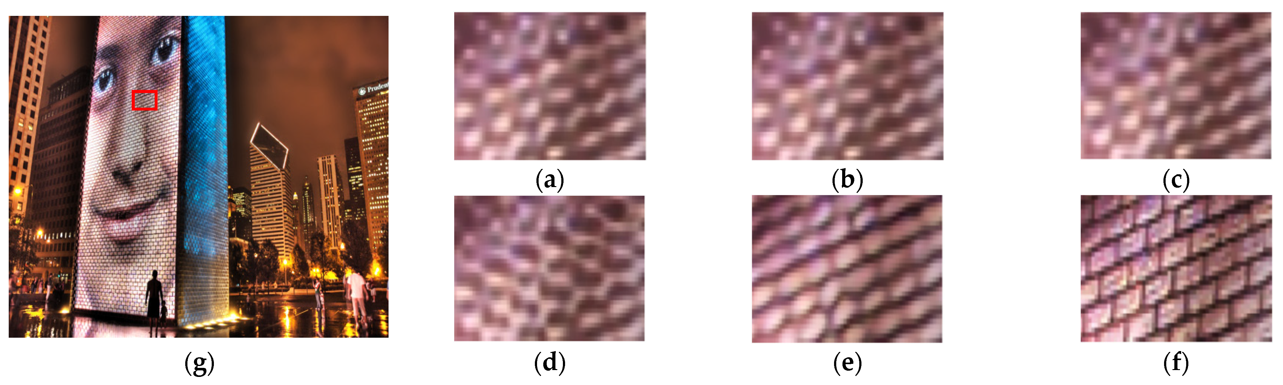
In Figure 9, VDSR [5], Lap-SRN [16,17], Meta-SR [21], and RCAN [19] all optimize details to reduce edge blur. From the overall picture, IDMF-SR and RCAN [19] have similar visual effects to the naked eye. In order to observe the pros and cons of each algorithm more clearly, we select some details of the image to upscale them, and observe the differences in image detail processing of each algorithm, as shown in Figure 9. There is a big difference in the restoration of the detail information of the image. The images (a)–(c) on Set14 img_005 are blurred. Compared with the previous methods, IDMF-SR has an improved reconstruction effect.
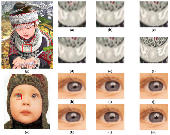
Figure 9.
The visual effect of each algorithm under ×2 upscale factor. (a) VDSR; (b) Lap-SRN; (c) Meta-SR; d) RCAN; (e) IDMF-SR (Ours); (f) HR (Original); (g) Set14 img_005 (2×); (h) VDSR; (i) Lap-SRN; (j) Meta-SR; (k) RCAN; (l) IDMF-SR (Ours); (m) HR (Original); (n) Set5 img_005 (2×).
3.3. Comparison of Model Parameters
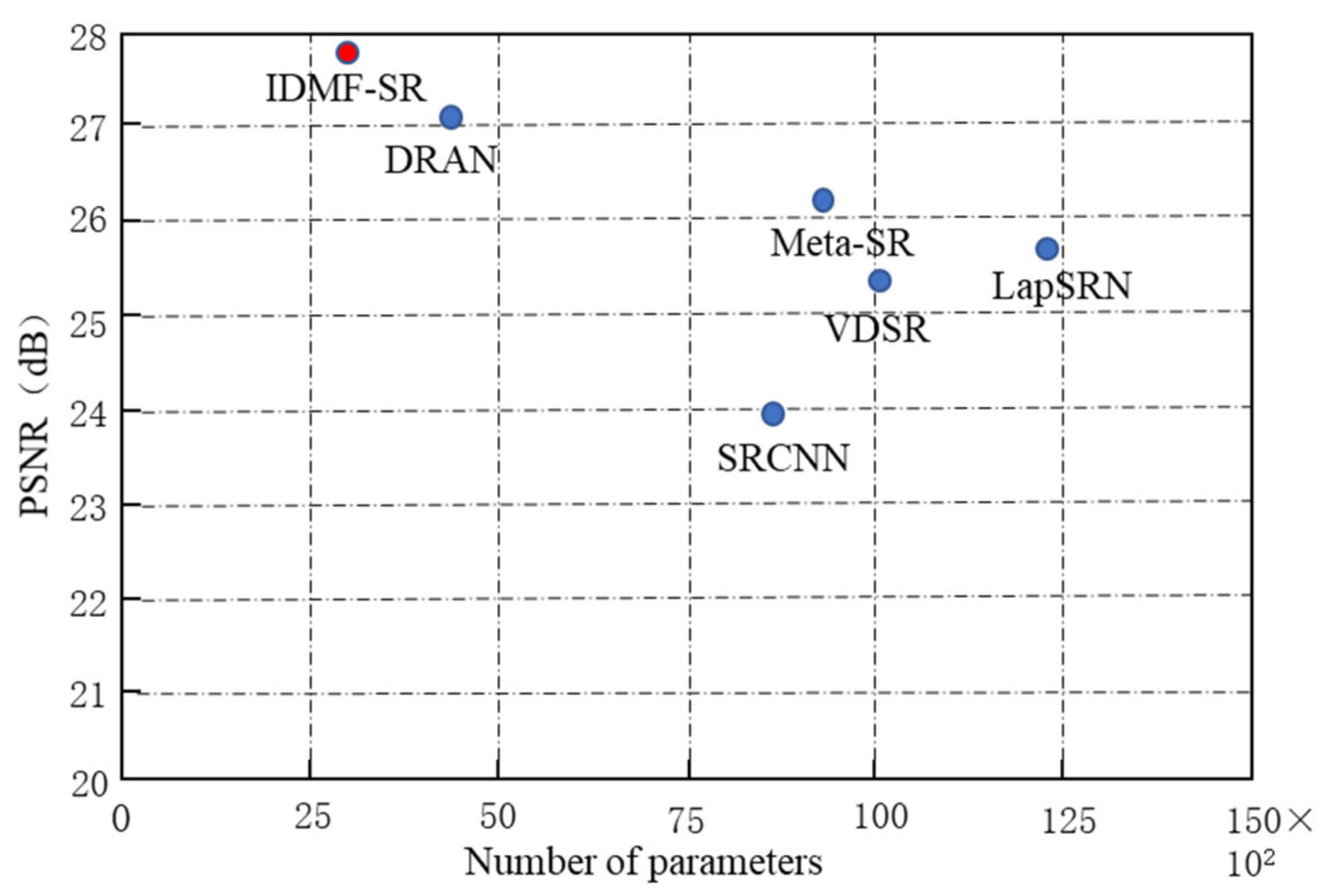
Compare the traditional algorithms and the IDMF-SR on the Urban100 test dataset Under ×4, the relationship between the average PSNR of the model and the parameter, as shown in Figure 10. The IDMF-SR proposed in this section changes the feature learning module based on Meta-SR [21], adopts an information distillation structure, progressively extracts image features, and cascades features. The feature does not fully participate in the next stage of the feature learning task. Therefore, only a few parameters can be used to achieve fast and accurate image super-resolution reconstruction, preventing parameter redundancy. It can be seen from Figure 10 that IDMF-SR has a 69.8% reduction in parameter quantity than Meta-SR [21] and a 2% increase in PSNR value. The algorithm in this section makes a trade-off between the number of model parameters and the PSNR value, which not only ensures the improvement of the SISR performance but also reduces the number of parameters.

Figure 10.
Multiple model PSNR value and parameter quantity relation diagram.
4. Discussion
Ablation Studies of IDM and CCAM
To quickly demonstrate the effect of the information distillation module (IDM) and contrast-based channel attention mechanism (CCAM), we remove the IDM between IDB and/or CCAM, so the IDMF-SR becomes the basis of a deep network, which we named IMDN-Basic, as described in Figure 11. Firstly, we use four IDB to certify the effect of IDM and CCAM. In Table 4, when both IDM and CCAM are removed, the PSNR on Set5 at the scale factor of 4 is 32.48 dB as the first column. When CCAM is added, the PSNR value reached 32.56 dB. This is because CCAM can improve the information about structures, textures, and edges that are propitious to enhance image details. The PSNR value reaches 32.62 dB with the contribution of IDM and CCAM. This indicates that IDM and CCAM are essential for improving SISR performance.
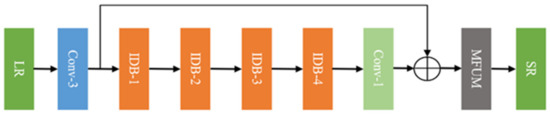
Figure 11.
IMDN-Basic. The grey box represents multi-factor upscaling module.
Table 4.
Investigations of CCA module and IIC scheme.
5. Conclusions
In this paper, we propose an information distillation structure to progressively extract multi-scale spatial features to achieve fast and accurate image super-resolution. The information distillation module divides the captured feature map into two parts. After each level of convolution, one third of the feature maps are retained and cascaded after the last convolutional layer. CCAM can further enhance image details, such as edges, textures, and structures. In addition, we propose a multi-factor upsampling module, which uses scale factors to predict filter weights. IDMF-SR can train a single model for super-resolution of arbitrary scale factor to achieve image super-resolution. Extensive experiments illustrate that the proposed IDMF-SR outperforms state-of-the-art versus SISR in terms of qualitative and quantitative evaluation.
Author Contributions
Project administration, S.C.; Validation, Z.L. and Y.C.; Visualization, N.Z. and Y.C.; Writing—original draft, Y.C.; Writing—review & editing, Y.C. and S.C. All authors have read and agreed to the published version of the manuscript.
Funding
This research received no external funding.
Institutional Review Board Statement
Not applicable.
Informed Consent Statement
Not applicable.
Data Availability Statement
Not applicable.
Conflicts of Interest
The authors declare no conflict of interest.
References
- Morin, R.; Basarab, A.; Kouamé, D. Alternating direction method of multipliers framework for super-resolution in ultrasound imaging. In Proceedings of the 2012 9th IEEE International Symposium on Biomedical Imaging (ISBI), Barcelona, Spain, 2–5 May 2012; pp. 1595–1598. [Google Scholar]
- LeCun, Y.; Bengio, Y.; Hinton, G. Deep Learning. Nature 2015, 521, 436–444. [Google Scholar] [CrossRef] [PubMed]
- Dong, C.; Loy, C.C.; He, K.; Tang, X. Learning a deep convolutional network for image super-resolution. In Proceedings of the European Conference on Computer Vision (ECCV), Zurich, Switzerland, 6–12 September 2014; pp. 184–199. [Google Scholar]
- Dong, C.; Loy, C.C.; He, K.; Tang, X. Image super-resolution using deep convolutional networks. IEEE Trans. Pattern Anal. Mach. Intell. 2016, 38, 295–307. [Google Scholar] [CrossRef] [PubMed] [Green Version]
- Kim, J.; Lee, J.K.; Lee, K.M. Accurate image super-resolution using very deep convolutional networks. In Proceedings of the IEEE Conference on Computer Vision and Pattern Recognition (CVPR), Las Vegas, NV, USA, 27–30 June 2016; pp. 1646–1654. [Google Scholar]
- Kim, J.; Lee, J.K.; Lee, K.M. Deeply-recursive convolutional network for image super-resolution. In Proceedings of the IEEE Conference on Computer Vision and Pattern Recognition (CVPR), Las Vegas, NV, USA, 20–30 June 2016; pp. 1637–1645. [Google Scholar]
- Tai, Y.; Yang, J.; Liu, X. Image super-resolution via deep recursive residual network. In Proceedings of the IEEE Conference on Computer Vision and Pattern Recognition (CVPR), Honolulu, HI, USA, 21–26 July 2017; pp. 2790–2798. [Google Scholar]
- Tai, Y.; Yang, J.; Liu, X.; Xu, C. MemNet: A Persistent Memory Network for Image Restoration. In Proceedings of the IEEE International Conference on Computer Vision (ICCV), Venice, Italy, 22–29 October 2017; Volume 43, pp. 2480–2495. [Google Scholar]
- Lim, B.; Son, S.; Kim, H.; Nah, S.; Mu Lee, K. Enhanced Deep Residual Networks for Single Image Super-Resolution. In Proceedings of the IEEE Conference on Computer Vision and Pattern Recognition Workshop (CVPRW), Honolulu, HI, USA, 22–25 July 2017; pp. 1132–1140. [Google Scholar]
- Zhang, Y.; Tian, Y.; Kong, Y.; Zhong, B.; Fu, Y. Residual Dense Network for Image Super-Resolution. In Proceedings of the IEEE Conference on Computer Vision and Pattern Recognition (CVPR), Nashville, TN, USA, 20–25 June 2021; Volume 43, pp. 2480–2495. [Google Scholar]
- Chen, J.; Huang, D.; Zhu, X.; Chen, F. Gradient-Guided and Multi-Scale Feature Network for Image Super-Resolution. Appl. Sci. 2022, 12, 62935. [Google Scholar] [CrossRef]
- Qin, J.; Liu, F.; Liu, K.; Jeon, G.; Yang, X. Lightweight hierarchical residual feature fusion network for single-image super-resolution. Neurocomputing 2022, 478, 104–123. [Google Scholar] [CrossRef]
- Wang, Z.; Chen, J.; Hoi, S.C. Deep Learning for Image Super-resolution: A Survey. IEEE Trans. Pattern Anal. Mach. Intell. 2021, 43, 3365–3387. [Google Scholar] [CrossRef] [PubMed] [Green Version]
- Kim, S.; Jun, D.; Kim, B.G.; Lee, H.; Rhee, E. Single Image Super-Resolution Method Using CNN-Based Lightweight Neural Networks. Appl. Sci. 2021, 11, 31092. [Google Scholar] [CrossRef]
- Dong, C.; Loy, C.C.; Tang, X. Accelerating the super-resolution convolutional neural network. In Proceedings of the European Conference on Computer Vision (ECCV), Amsterdam, The Netherlands, 8–16 October 2016; pp. 391–407. [Google Scholar]
- Lai, W.S.; Huang, J.B.; Ahuja, N.; Yang, M.H. Deep laplacian pyramid networks for fast and accurate super-resolution. In Proceedings of the IEEE Conference on Computer Vision and Pattern Recognition (CVPR), Honolulu, HI, USA, 21–26 July 2017; pp. 5835–5843. [Google Scholar]
- Lai, W.S.; Huang, J.B.; Ahuja, N.; Yang, M.H. Fast and Accurate Image Super-Resolution with Deep Laplacian Pyramid Networks. IEEE Trans. Pattern Anal. Mach. Intell. 2019, 41, 2599–2613. [Google Scholar] [CrossRef] [PubMed] [Green Version]
- Shi, W.; Caballero, J.; Huszár, F.; Totz, J.; Aitken, A.P.; Bishop, R.; Rueckert, D.; Wang, Z. Real-time single image and video super-resolution using an efficient sub-pixel convolutional neural network. In Proceedings of the IEEE Conference on Computer Vision and Pattern Recognition, Las Vegas, NV, USA, 27–30 June 2016; pp. 1874–1883. [Google Scholar]
- Zhang, Y.; Li, K.; Li, K.; Wang, L.; Zhong, B.; Fu, Y. Image Super-resolution Using Very Deep Residual Channel Attention Networks. In Proceedings of the European Conference on Computer Vision (ECCV), Munich, Germany, 8–14 September 2018; pp. 1328–1344. [Google Scholar]
- Tian, C.; Zhuge, R.; Wu, Z.; Xu, Y.; Zuo, W.; Chen, C.; Lin, C.W. Lightweight Image Super-Resolution with Enhanced CNN. Neurocomputing 2020, 205, 106235. [Google Scholar] [CrossRef]
- Hu, X.; Mu, H.; Zhang, X.; Wang, Z.; Tan, T.; Sun, J. Meta-SR: A Magnification-Arbitrary Network for Super-Resolution. In Proceedings of the 2019 IEEE/CVF Conference on Computer Vision and Pattern Recognition (CVPR), Long Beach, CA, USA, 15–20 June 2019; pp. 1575–1584. [Google Scholar]
- Bevilacqua, M.; Roumy, A.; Guillemot, C.; Alberi-Morel, M.L. Low-complexity single-image super-resolution based on nonnegative neighbor embedding. In Proceedings of the British Machine Vision Conference (BMVC), Surrey, UK, 3–7 September 2012. [Google Scholar]
- Zeyde, R.; Elad, M.; Protter, M. On single image scale-up using sparse representations. In Proceedings of the International Conference on Curves and Surfaces (ICCS), Avignon, France, 24–30 June 2010; pp. 711–730. [Google Scholar]
- Martin, D.; Fowlkes, C.; Tal, D.; Malik, J. A database of human segmented natural images and its application to evaluating segmentation algorithms and measuring ecological statistics. In Proceedings of the International Conference on Computer Vision (ICCV), Vancouver, BC, Canada, 7–14 July 2001; pp. 416–423. [Google Scholar]
- Matsui, Y.; Ito, K.; Aramaki, Y.; Fujimoto, A.; Ogawa, T.; Yamasaki, T.; Aizawa, K. Sketch-based manga retrieval using manga109 dataset. Multimed. Tools Appl. 2017, 76, 21811–21838. [Google Scholar] [CrossRef] [Green Version]
- Kim, J.; Shin, M.; Kim, D.; Park, S.; Kang, Y.; Kim, J.; Lee, H.; Yun, W.J.; Choi, J.; Park, S.; et al. Performance Comparison of SRCNN, VDSR, and SRDenseNet Deep Learning Models in Embedded Autonomous Driving Platforms. In Proceedings of the 2021 International Conference on Information Networking (ICOIN), Jeju Island, Korea, 13–16 January 2021; pp. 56–58. [Google Scholar]
- Wang, Z.; Bovik, A.C.; Sheikh, H.R.; Simoncelli, E.P. Image quality assessment: From error visibility to structural similarity. IEEE Trans. Image Process. 2004, 13, 600–612. [Google Scholar] [CrossRef] [PubMed] [Green Version]


Publisher’s Note: MDPI stays neutral with regard to jurisdictional claims in published maps and institutional affiliations. |
© 2022 by the authors. Licensee MDPI, Basel, Switzerland. This article is an open access article distributed under the terms and conditions of the Creative Commons Attribution (CC BY) license (https://creativecommons.org/licenses/by/4.0/).