
Multilayer Dielectric Periodic Antenna Structure in a Cascade View

Faculty Electronics, Military University of Technology, 00-908 Warsaw, Poland
Appl. Sci. 2022, 12(9), 4185; https://doi.org/10.3390/app12094185
Submission received: 23 March 2022
/
Revised: 16 April 2022
/
Accepted: 18 April 2022
/
Published: 21 April 2022
(This article belongs to the Special Issue Advances in Analytical-Numerical Techniques for Planar Microwave Circuits and Microstrip Antennas)
Abstract
:The spectral response of the periodic antenna structure placed in a dielectric homogeneous medium depends on the antenna geometry, the parameters of the medium, the angle of incidence, polarization, and the geometry of the excitation field. Increasing the number of antenna structure parameters can be achieved by introducing a multilayer dielectric medium with a certain number of metallized periodic surfaces located on flat boundaries between the dielectric layers. There are two complementary approaches to the analysis of such structures. In the first, the composite antenna system is analysed by constructing supermodes of the entire structure. In the second, the system is considered as a cascade assembly of flat discrete elements, i.e., the boundaries between two dielectrics, periodic metallized planes, and dielectric layers. The latter approach leads to the definition of the scattering, transmission, or impedance matrix of the entire structure by cascading the corresponding matrices associated with the individual discrete elements of the antenna structure. It is particularly useful in modelling dielectric multilayer antenna walls, where the stored data on one planar antenna element can be used many times in the analysis of various antenna systems with modified parameters of other discrete structure elements. Microstrip antennas combine field and peripheral problems and require the use of analytical methods of a high degree of complexity. Therefore, at present, there are no standard methods that can be used in engineering practice. This work is a step towards filling these gaps.
1. Introduction
The spectral response of the periodic antenna structure placed in a dielectric homogeneous medium depends on the antenna geometry, the parameters of the medium, the angle of incidence, polarization, and the geometry of the excitation field. However, in many applications, the above number of parameters determining the operation of the antenna is not sufficient to be able to model its desired directional characteristics. Increasing the number of antenna structure parameters can be achieved by introducing a multilayer dielectric medium with a certain number of metallized periodic surfaces located on flat boundaries between the dielectric layers [1,2]. The analysis of such a multilayer planar antenna system is the subject of this work. There are two complementary approaches to the analysis of such structures. In the first, the composite antenna system is analysed by constructing supermodes of the entire structure. In the second, the system is considered as a cascade assembly of flat discrete elements, i.e., the boundaries between two dielectrics, periodic metallized planes, and dielectric layers [3]. The latter approach leads to the definition of the scattering, transmission, or impedance matrix of the entire structure by cascading the corresponding matrices associated with the individual discrete elements of the antenna structure. It is particularly useful in modelling dielectric multilayer antenna walls, where the stored data on one planar antenna element can be used many times in the analysis of various antenna systems with modified parameters of other discrete structure elements.
In practice, antenna arrays most often consist of periodic metal structures placed on or immersed in a dielectric multilayer medium. Changes in the size and shape of individual antenna elements enable efficient modeling of its spectral parameters. These changes can be additionally modeled by selecting the geometrical and physical parameters of the dielectric layered substrate and coating. In the case of large transverse dimensions, the antenna is in the order of 100 wavelengths and several dozen or more individual metal radiation elements. The radiation properties of the antenna approximately correspond to those of the unlimited antenna structure. Under the condition of periodicity of such an antenna and its excitation with linear, homogeneous phase modulation, the problem of scattering on such a structure comes down to the analysis of one basic antenna cell, usually in a spectral space spanned by a complete array of corresponding Floquet harmonics. For structures of smaller sizes and fewer elements, the effects related to their limitations, especially the edge effects occurring on their outer cells, may affect the antenna performance characteristics and should be considered in their modeling. So far, there is no known exact effective method for solving the scattering problem on such periodic constrained structures. Attempts to solve this problem by directly applying the spectral method of moments are only formally strict. This is because their accuracy is limited by the constraints imposed on the size of the matrices used in the procedures for solving them. Nevertheless, for antenna walls composed of a few or a dozen regular-shaped basic cells, this method gives good results. Other known methods of solving the scattering problem on larger periodic structures, such as modifications of the above-mentioned direct method by limiting the number of base functions and appropriate selection of their waveforms, or the iterative method imposed on the solution by successive application of the Fast Fourier transform, are approximate, slow convergent, and can only be used in some simple, easy-to-analyze cases. Currently, a computer program is being developed that will allow verification of the adopted assumptions.
The generalized scattering matrix method was originally used in the analysis of waveguide problems, considering both propagating and vanishing [4]. Treating the composite antenna array as a waveguide with many planar discontinuities, a similar analysis can also be applied to antenna theory. This method is applied in this work to multilayer periodic systems in one or two directions.
2. Statement of the Problem
We consider the composite periodic antenna structure shown in Figure 1. The system consists of many-layered elements bounded at the top and bottom by half-spaces (upper and lower) of homogeneous dielectric media. The third axis (y) of the orthogonal coordinate system (x,y,z) is perpendicular to the drawing plane. The basic components of the structure are: metallized, infinitely periodic in the plane (x,y) antenna surface, the boundary between two dielectrics, and a homogeneous dielectric layer [5,6].
The periodic flat antenna structure is shown in Figure 1. The geometry of a single antenna element remains arbitrary. The distance between the individual antenna elements in the x and y directions is dx and dy, respectively. The inclination angles of the symmetry axis of the antenna structure with respect to the x axis are respectively 0 and . Let us assume that the designations of the multi-layer antenna system are shown in Figure 2.
The matrix S(j) or T(j) represents the planar discrete element of the antenna in the form of a flat metallized grid, a boundary between two dielectric media or a dielectric layer [7]. It was assumed that .
Vectors, , are the complex amplitudes of the normalized incoming and outgoing discrete modes of a single structure, represented by a scattering matrix S(j), or a transmission matrix T(j). The matrix S(j), binds the outgoing modes with falling modes
and matrix T connects the field on the “right ”, lower side of the structure with the field on the “left”, upper side of the structure:
Both types of matrices lead to a global description of the operation of the entire antenna structure [8]. Global transmission matrix T
has the form of a cascade assembly of individual elements of the antenna structure, which corresponds to the product of the transmission matrix of individual structure elements:
Knowing the matrices T(j) and T, it is possible to determine the matrices S(j) and S according to the formula:
Then we determine the global transmission matrix by the product of successive partial transmission matrices. Thus, for the determination of the scattering matrices it is practically necessary also to determine the partial and global transmission matrices. Similarly, knowing the form of the scattering matrices S(j) of individual elements of the structure, the matrices T(j) can be determined according to the formula:
and hence we also obtain the global transmission matrix T as a product of the matrix T(j) [7].
In general, the cut-off numbers Kj of an infinite countable number of modes of a structure may change from one subsystem of the structure to another, i.e., they may depend on the number j. For the simplicity of notation and further numerical implementation, however, assume that Kj = const. for any subsystem j = 1, 2,… J, which is also commonly used in numerical calculations. So we assume that the matrices S(j) and T(j) are square of the order 2K and the matrices S(j)kl, T(j)kl, k, l = 1, 2 are of the order K [9]. Particular antenna subsystems, as well as the entire antenna system, can also be expressed by impedance matrices Z(j) or admittance matrices Y(j) according to the following formulas [4,5] ([S] ≡ S):
where: [ς0] diagonal matrix of characteristic impedances.
The form of the matrix S, T, Z, or Y depends on the geometry and parameters of the antenna structure medium, as well as on the adopted complete base of eigenvectors of the appropriate boundary problem. The electromagnetic field at any point in the structure is presented in the form of Fourier integrals or series with appropriate, generally complex, coefficients (amplitudes) of the distribution [10,11]. For infinite periodic structures, the equivalent of Fourier transforms is the field distributions to Floquet’s harmonics. As a result, the transverse electric field Et is presented in the form of a series:
where denote the coefficients of the field distribution propagating in a positive (+) or negative (−) direction with a phase factor . The vectorial normalized to the unit power of Floquet’s harmonics Ψk, defined in the next subsection, have a phase factor ek(x,y) and vector amplitudes ψk. The index k follows TE or TM polarization and the generally infinite Floquet harmonics indices in the x(m) and y(n) directions [12]. Similarly, for the transverse magnetic field we get:
where: ηq denotes the harmonic modal impedance with index q. With the normalization of the power of individual harmonics adopted below, the total field power flux in the z direction is expressed by the amplitude modulus vk:
where the summation along the index k runs both the propagating modes (Im(kzk) = 0) and vanishing modes (Im(kzk) ≠ 0) [13].
3. Modes of the Planar Endless Bidinary Periodic Structure Scalar Harmonics of Floquet
Let us consider the function f(x,y) periodically depending on x and y with the accuracy to the linear phase factor φx + φy:
where dx and dy are lattice constants in the plane (x,y) and the function f(x,y) satisfies the Helmholtz equation in space (x,y) [2]:
Moreover, the longitudinal components kz and the transverse components kx and ky of the propagation vector satisfy the dispersion equation: .
The above definition of the function f(x,y) shows that the function F(x,y) = f(x,y) exp[i(φxx/dx + φyy/dy)] is periodic, i.e., it satisfies the condition F(x + dx,y + dy) = F(x,y) and as such can be represented as a typical Fourier series:
Hence the pseudo-periodic function f(x,y) is represented in the form of a distribution [14]
for Floquet harmonics:
with the coefficients of the Amn. distribution. The form of the components of the propagation vector k reflects the periodic symmetry of the problem under consideration along the x and z axes:
Note that the transverse component (in the x,y plane) of the wave vector is:
The above distribution is a generalization of the Fourier series of the pseudo-periodic function f(x,y) with linear phase increment (mφx + nφy) for translation (mx + ny) in the transverse plane (x,y) [15] For a two-dimensional periodic structure with the inclination angle Ω of the second symmetry axis with respect to the x axis (the remaining symmetry axis coincides with the x axis), we get:
In the general case, for any position of the axis of symmetry with respect to the axis of orthogonal coordinates x and y, all three components of the propagation vector kxmn, kymn, kzmn depend on both m and n. We then make these components dependent on the wave vector of the zero (m = n = 0) harmonics Floquet of the incident field
where θinc and φinc. denote the angles of incidence in the planes (z,y) and (x,y), respectively. Then the phase shifts φx, φy for the translation of dx, dy by one periodic cell are respectively:
Without losing the generality of considerations, let us then assume that all individual components (j) of the layered antenna structure are defined with respect to the upper outer center, i.e., the incidence center. Then, for any j, from the continuity of the tangent components Et = (Ex,Ey), Ht = (Hx,Hy) in the planes of discontinuity z = zj = const. it follows that the transverse and correspond to the transverse components of the wave vector in the following form:
kx00, ky00 components of the Floquet harmonic wave vector of the zero spectral cell (m = 0, n = 0) remain equal to the corresponding component in the incidence center:
The above property holds true for any j, i.e., for each individual element of the composite antenna structure. In other words, the components kx00, ky00 remain independent of z. Similarly, for any values of m and n, i.e., for harmonics of any order, we get:
Let us then proceed to deriving the representation for the transverse components of the electromagnetic field in the form of the distribution into Floquet vector harmonics.
4. Vector Harmonics of Floquet—Electromagnetic Field Representation in the Plane (x,y)
The electromagnetic field at any point of the previously defined multi-layer antenna structure can be decomposed into two independent field components distinguished by their polarization with respect to the antenna plane normal, i.e., TE field with an electric field vector perpendicular to the z direction: E(x,y,z) = (Et,Ez) and the TM field with the magnetic field vector perpendicular to the z direction: H(x,y,z) = (Ht,Hz). As part of this division, we will define the distributions of the transverse electric field into vector Floquet harmonics, characterizing the mode structure of the electromagnetic field of an unlimited, multi-layer periodic structure. It should be noted that with the assumed losslessness of the upper (incident) medium, the above-analyzed tangents (to the (x,y) plane) coordinates of the propagation vector corresponding to the incident field harmonics remain real in every element of the antenna structure, both lossy and lossless.
4.1. TE Polarization
For the TE field, let us assume that the longitudinal component of the magnetic field HzTEmn as a pseudo-periodic function f(x,y) with the appropriate phase factor depending on z:
From Maxwell’s equations, the electric transverse field EtTEmn = (ExTEmn, EyTEmn) is expressed through the field HzTEmn [16] as follows:
where: nx, ny, nz denote the unit vectors along the respective x, y, and z axes. In further considerations, we will also denote the sequence of TEmn or TMmn pointers with one symbol from the set {q,p}. Let us introduce the orthogonal and normalized Floquet vector harmonics Ψq (q = Ψq (q = TEmn)), i.e., satisfying the condition:
where integration takes place over a single elementary cell of a periodic structure with the surface of S. The normalized Floquet harmonics contain, in addition to the phase factor
also normalizing vector amplitude coefficient:
Thus, Floquet’s vector harmonics take the following form:
with coordinates in the x and y directions, respectively:
Finally, the transverse electric field with a polarization TE Etq (q = TEmn) is defined as proportional to the transverse vector harmonic Ψtq:
and the longitudinal component Htq of the magnetic field with a polarization TE is determined from the knowledge of the transverse electric field Etq
and using the mode impedance ηq of a harmonic with a polarization TE.
The factor (ηq*)1/2 standing at the normalized vector harmonic Ψq provides the normalization of the power of the harmonic field, which corresponds to the unit power flow conducted through this harmonic in the direction of the z axis:
4.2. TM Polarization
For the TM field, let us take the longitudinal component of the electric field EzTMmn as the functions f(x,y) with the appropriate phase factor depending on z:
Transverse fields: magnetic HtTMmn = (HxTMmn, HyTMmn) and electric EtTMmn = (ExTMmn, EyTMmn) are expressed through the EzTMmn field as follows [6,17]:
Let us introduce the orthonormal vector harmonics of Floquet [18]: ΨTMmn ≡ Ψp (p = TMmn) about TM polarization
that is
Then, analogically to the case of TE polarization, the orthogonality relationship takes place:
Additionally, TE modes remain orthogonal to TM modes:
which leads to the relationship of orthogonality in the general form (p, q run for any values from the sets {TE, TM}, {m}, {n}):
Then, considering the mode impedance for the polarization we finally obtain the form of the transverse components [19] of the electric field Etp and magnetic Htp with TM polarity (p = TMmn):
Hence the transverse magnetic field Htp is expressed by vector harmonics Htp in the following way:
The coefficient (ηp)−1/2 at the normalized vector harmonic nz × Ψp ensures the normalization of the harmonic field power with the polarization TM:
5. General Dispersion Material for Individual Composite Antenna Structure
Based on the mode structure defined in the previous section, the electromagnetic field of the composite antenna can, for any of the following, be presented in the form of a series:
with the known vector Floquet harmonics Ψk and the distribution coefficients remaining to be determined [20,21]. Given the known field incident on the antenna, determining the total field requires deriving the scattering matrix of the entire system. The solution is obtained by determining the scattering matrix of individual planar system elements, such as the dielectric boundary, metallized periodic plane, and a layer of a homogeneous dielectric medium. In each of these cases, the distribution coefficients correspond to the field amplitudes defined in Figure 2.
Let us consider any single element of a composite antenna denoted by the index j. Let us create a vector Vj(in) of field amplitudes entering (in) into the system (j), which in turn consists of a vector Vj(inup) of amplitudes of type in on the upper (upper) side of the system (j) and the vector Vj(inlow) of amplitudes of type in from the lower side of the system (j):
Similarly, we define the vector Vj(ou) of field amplitudes coming from the system (j):
The definition of the relationship between these two vectors is determined by the scattering matrix S(j):
So the vector Vj(in) consists of an infinite sequence of amplitudes from the top of the element (j), vk—from the bottom of the element (j), and the vector Vj(ou)—from the sequences of the respective amplitudes and
Inequalities mean, conventionally, the top and bottom side of a single antenna element. For example, for the dielectric boundary and the periodic plane, this means limδ→0 (zj ± δ), respectively. In numerical calculations, the vectors Vj(in), Vj(ou) with an infinite number of parameters are usually cut to 2 (M + N) elements, where the number 2 corresponds to the two polarizations TE and TM, M—the number of harmonics in the x direction, and N—the number of harmonics in the y direction. It follows that S (j) kl, k, l = 1.2 are of the order of 2MN. In order to determine the global matrix S, it is necessary to know the scattering matrix of individual system elements. These include the metallized periodic plane, the dielectric boundary, and the homogeneous dielectric layer.
6. Plane with Endlessly Metal Periodic Mesh
The geometry of the periodic plane is presented in Figure 1. The geometry of a single periodic cell is arbitrary. As a result of the scattering analysis on such a structure (using the spectral variant of the Galerkin method) [22], we obtain an equation linking the vector of the scattered field amplitudes Vjs with the field amplitude vector incident on the periodic structure Vj(inup):
where Vji ≡ Vj (inup), matrix I denotes the identity matrix, Γ—the reflection matrix from the periodic surface, M—the matrix of conjugate coefficients of the distribution of base functions into Floquet harmonics, and the W and U matrices are determined by the Fourier transform of the Green function of the surrounding medium and the base functions used in the Galerkin method.
For the incident field Vji then we get:
What from the asymmetry of the reflection coefficient on the dielectric boundary and the continuity of the field tangent components on the boundary of two dielectrics gives the following matrix form S(j):
6.1. Dielectric Limit
The scattering matrix of the dielectric boundary meets the conditions of anti-reciprocity:
and it is symmetrical
and the individual sub-matrices of the scattering matrices correspond to the reflection matrices R(j) and transmission T(j).
The R(j) and T(j) reflection matrices have zero elements outside the diagonals, which means that there is no coupling between the different field harmonics (in the isotropic case considered here). The diagonal elements of these matrices are expressed by the mode impedances ηk(up) and ηk(low) of the harmonics Ψk propagating in the upper and lower centers, respectively:
6.2. Dielectric Layer
The remaining element of the structure (the dielectric layer) corresponds to the propagation of individual harmonics in the dielectric medium (let’s assume bj) without coupling between the harmonics. The scattering matrix of such a (homogeneous, isotropic) dielectric layer also has only non-zero elements on the diagonal and they are expressed by the appropriate field phase change for propagating harmonics or a field amplitude change for disappearing harmonics:
7. Cascade Assembly of the Individual Elements of the Composite Antenna
Knowing the scattering matrices S(j) of individual elements of the system, the global matrix S is determined according to the scheme presented in point 2. So for each element of the antenna structure, we determine the transmission matrix corresponding to this element.
Then we determine the global transmission matrix by the product of successive partial transmission matrices:
and then we calculate the global scattering matrix according to the formula:
8. Conclusions
According to the procedure given above, it is practically necessary to determine the partial and global transmission matrices for the determination of the scattering matrices. In the case of specific antenna structures, various modifications of the above analysis are applied in order to obtain faster convergence of the applied numerical procedure and limitations on the memory capacity requirements used by the numeric program. Extremely important from the point of view of the effectiveness and accuracy of the procedure is the selection of the number of truncation K of harmonics included in the numerical calculations and their order in the series of the field distribution. Usually, the order of harmonics is determined by the increase in the value of their propagation constants. The value of the number K depends on the characteristic transverse and longitudinal distances that are normalized to the refractive index of the medium. The rule is that the smaller the distances between the individual cells of the periodic plane, the higher the harmonics should be considered in the field distribution, including also the decaying modes, especially important at small distances between individual planar antenna elements. The proposed solution enables the analysis of antenna arrays located on a multilayer dielectric. The presented procedure for the solution of electromagnetic field scattering on the antenna array is the original solution. Based on the derived dependencies, a computer program will be developed to analyze the parameters and characteristics of this type of antenna.
Funding
This research was funded by Military University of Technology, Faculty of Electronics, grant number 22-738.
Informed Consent Statement
Not applicable.
Data Availability Statement
Not applicable.
Conflicts of Interest
The author declares no conflict of interest.
References
- Kong, J.A. Electromagnetic Wave Theory; EMW Publishing: Cambridge, MA, USA, 2008. [Google Scholar]
- Sadiku, M.N. Elements of Electromagnetics; Oxford University Press: Oxford, UK, 2014. [Google Scholar]
- Lancaster, T.; Blundell, S.J. Quantum Field Theory for the Gifted Amateur; OUP Oxford: Oxford, UK, 2014. [Google Scholar]
- Bender, C.M.; Orszag, S.A. Advanced Methods for Scientists and Engineers I: Asymptotic Methods and Perturbation Theory; Springer Science & Business Media: Berlin/Heidelberg, Germany, 2013. [Google Scholar]
- Balanis, C. Advanced Engineering Electromagnetics; Wiley: Hoboken, NJ, USA, 2012. [Google Scholar]
- Balanis, C.A. Antenna Theory: Analysis and Design; John Wiley & Sons: Hoboken, NJ, USA, 2016. [Google Scholar]
- Oppenheim, A.V.; Schafer, R.W. Electromagnetic Field Theory Discrete-Time Signal Processing; Pearson Education: London, UK, 2014. [Google Scholar]
- Chuang, S.L. Physics of Photonic Devices; John Wiley & Sons: Hoboken, NJ, USA, 2012; Volume 80. [Google Scholar]
- Born, M.; Wolf, E. Principles of Optics: Electromagnetic Theory of Propagation, Interference and Diffraction of Light; Elsevier: Amsterdam, The Netherlands, 2013. [Google Scholar]
- Chew, W.C. Quantum Mechanics Made Simple: Lecture Notes for ECE 487 at UIUC. Available online: http://wcchew.ece.illinois.edu/chew/course/QMAll20161206.pdf (accessed on 6 December 2016).
- Imbriale, W.A.; Gao, S.S.; Boccia, L. Space Antenna Handbook; John Wiley & Sons: Hoboken, NJ, USA, 2012. [Google Scholar]
- Smithsonian. This 1600-Year-Old Goblet Shows that the Romans Were Nanotechnology Pioneers. Available online: https://www.smithsonianmag.com/history/this-1600-year-old-goblet-shows-that-the-romans-were-nanotechnology-pioneers-787224/ (accessed on 6 September 2019).
- Chew, W.C. Lectures on Theory of Microwave and Optical Waveguides. For ECE 531 at UIUC. Available online: https://engineering.purdue.edu/wcchew/course/tgwAll20160215.pdf (accessed on 24 July 2021).
- Liu, Q.S.; Sun, S.; Chew, W.C. A potential-based integral equation method for low-frequency electromagnetic problems. IEEE Trans. Antennas Propag. 2018, 66, 1413–1426. [Google Scholar] [CrossRef]
- Glytsis, E. Slab Waveguide Fundamentals. Available online: http://users.ntua.gr/eglytsis/IO/users.ntua.gr/eglytsis/IO/Slab_Waveguides_Chapter.pdf (accessed on 19 November 2020).
- Chew, W.C.; Sha, W.; Dai, Q.I. Green’s Dyadic, Spectral Function, Local Density of States, and Fluctuation Dissipation Theorem. arXiv 2015, arXiv:1505.01586. [Google Scholar] [CrossRef] [Green Version]
- Yaghjian, A.D. Reflections on Maxwell’s treatise. Prog. Electromagn. Res. 2014, 149, 217–249. [Google Scholar] [CrossRef] [Green Version]
- Minatti, G.; Faenzi, M.; Martini, E.; Caminita, F.; de Vita, P.; Gonz’alez-Ovejero, D.; Sabbadini, M.; Maci, S. Modulated metasurface antennas for space: Synthesis, analysis and realizations. IEEE Trans. Antennas Propag. 2014, 63, 1288–1300. [Google Scholar] [CrossRef]
- Gao, X.; Han, X.; Cao, W.-P.; Li, H.O.; Ma, H.F.; Cui, T.J. Ultrawideband and high-efficiency linear polarization converter based on double v-shaped metasurface. IEEE Trans. Antennas Propag. 2015, 63, 3522–3530. [Google Scholar] [CrossRef]
- Zhan, Q. Cylindrical vector beams: From mathematical concepts to applications. Adv. Opt. Photonics 2009, 1, 1–57. [Google Scholar] [CrossRef]
- Saleh, B.E.; Teich, M.C. Fundamentals of Photonics; John Wiley & Sons: Hoboken, NJ, USA, 2019. [Google Scholar]
- Courant, R.; Hilbert, D. Methods of Mathematical Physics: Partial Differential Equations; John Wiley & Sons: Hoboken, NJ, USA, 2008. [Google Scholar]
Figure 1.
Flat periodic antenna structure infinite in the (x,y) plane, multilayer structure.
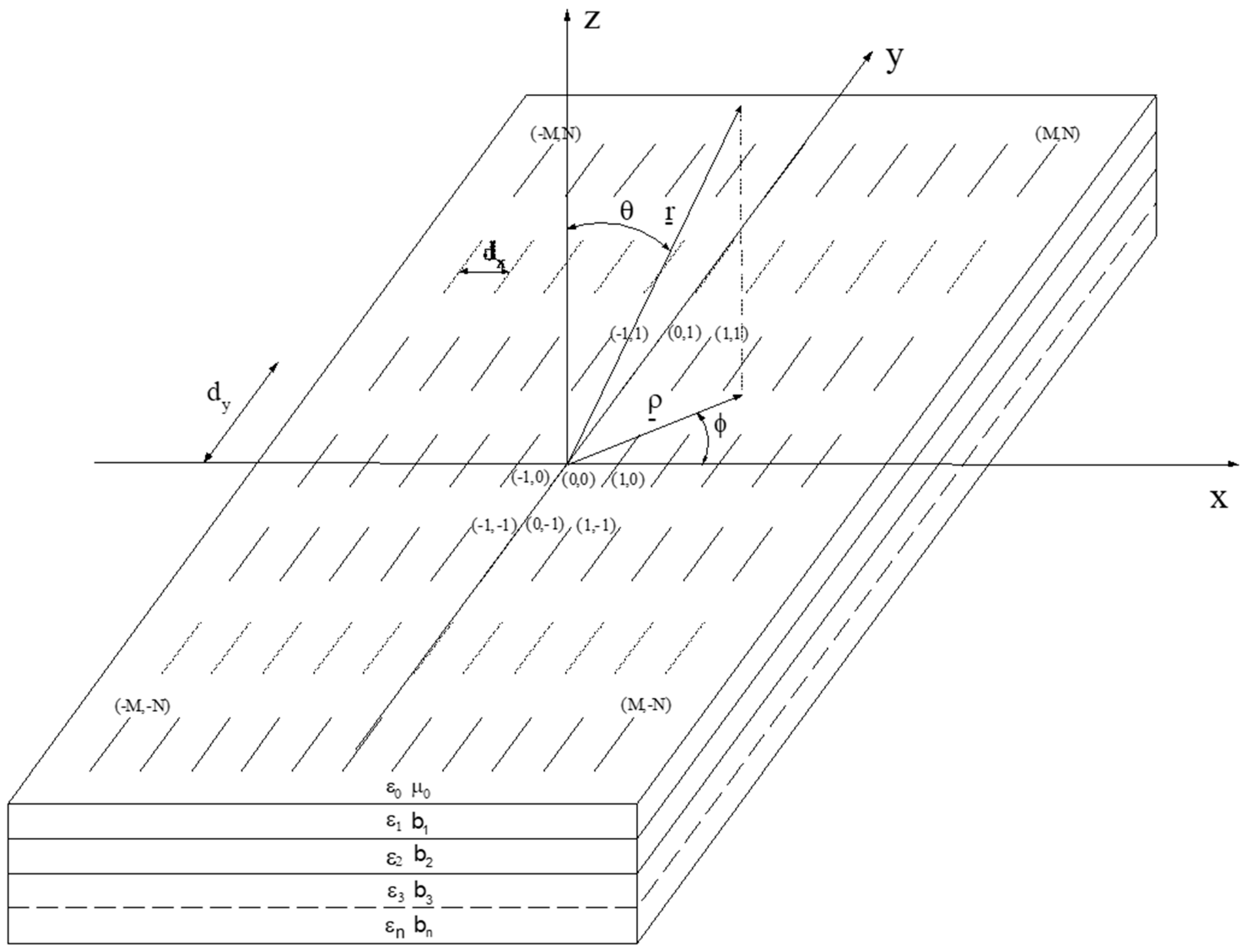
Figure 2.
Block diagram of a multi-layer antenna.

Publisher’s Note: MDPI stays neutral with regard to jurisdictional claims in published maps and institutional affiliations. |
© 2022 by the author. Licensee MDPI, Basel, Switzerland. This article is an open access article distributed under the terms and conditions of the Creative Commons Attribution (CC BY) license (https://creativecommons.org/licenses/by/4.0/).
Share and Cite
MDPI and ACS Style
Wnuk, M. Multilayer Dielectric Periodic Antenna Structure in a Cascade View. Appl. Sci. 2022, 12, 4185. https://doi.org/10.3390/app12094185
AMA Style
Wnuk M. Multilayer Dielectric Periodic Antenna Structure in a Cascade View. Applied Sciences. 2022; 12(9):4185. https://doi.org/10.3390/app12094185
Chicago/Turabian StyleWnuk, Marian. 2022. "Multilayer Dielectric Periodic Antenna Structure in a Cascade View" Applied Sciences 12, no. 9: 4185. https://doi.org/10.3390/app12094185
Note that from the first issue of 2016, this journal uses article numbers instead of page numbers. See further details here.