Tire Contact Force Equations for Vision-Based Vehicle Weight Identification

Abstract

Overloaded vehicles have a variety of adverse effects; they not only damage pavements, bridges, and other infrastructure but also threaten the safety of human life. Therefore, it is necessary to address the problem of overloading, and this requires the accurate identification of the vehicle weight. Many methods have been used to identify vehicle weights. Most of them use contact methods that require sensors attached to or embedded in the road or bridge, which have disadvantages such as high cost, low accuracy, and poor durability. The authors have developed a vehicle weight identification method based on computer vision. The methodology identifies the tire–road contact force by establishing the relationship using the tire vertical deflection, which is extracted using computer vision techniques from the tire image. The focus of the present paper is to study the tire–road contact mechanism and develop tire contact force equations. Theoretical derivations and numerical simulations were conducted first to establish the tire force–deformation equations. The proposed vision-based vehicle weight identification method was then validated with field experiments using two passenger cars and two trucks. The effects of different tire specifications, loads, and inflation pressures were studied as well. The experiment showed that the results predicted by the proposed method agreed well with the measured results. Compared with the traditional method, the developed method based on tire mechanics and computer vision has the advantages of high accuracy and efficiency, easy operation, low cost, and there is no need to lay out sensors; thus, it provides a new approach to vehicle weighing.

1. Introduction

The development of the transportation industry has led to an increase in overloaded vehicles. Overloaded vehicles can easily cause damage and the failure of bridges and pavements [1,2,3]. Although research to identify overloaded vehicles has been ongoing for many years, there is still no convenient and effective method to identify the vehicle weight accurately.

Existing methods to estimate the vehicle weight include the static weighing method and the weigh-in-motion (WIM) method. The static weighing method, which uses a load meter to measure the weight of stationary vehicles, is a standard method at present with obvious drawbacks: high cost and it causes traffic congestion [4,5]. WIM methods mainly include the pavement-based weigh-in-motion (PWIM) method and the bridge weigh-in-motion (BWIM) method. The PWIM method needs the sensors to be embedded in the road to identify the speed, axle spacing, and weight of moving vehicles. However, the vehicle load acts on sensors directly and constantly, resulting in the poor durability, short service life, and high maintenance cost of the system [6,7]. The BWIM method proposed by Moses in 1979, aims to calculate the vehicle weight by measuring the dynamic response of the bridge under the action of moving vehicles [8]. Yu et al. [9] and Lydon et al. [10] discussed the standard algorithms of BWIM in detail, and summarized its current progress and critical challenges. Compared with the static weighing and the PWIM methods, the BWIM method has the advantages of lower loss to sensors, longer service life, and no traffic interruption. However, the BWIM method requires the measurement of bridge response by installing sensors at the bridge bottom, which is difficult or inconvenient for cases such as an overpass or river-crossing bridges. Besides, the accuracy of the BWIM method is susceptible to the environment, and only applicable to short- and medium-span bridges.

In the past few years, computer vision become a popular technology that has been widely used in various research fields. It has the advantages of low cost, non-contact, ease of setup and operation, and the flexibility of multipoint detection, which is very useful for the temporal and spatial identification of moving vehicles; thus it also provides a new method for vehicle weight identification. Chen et al. [11] proposed an approach to identify the spatio-temporal distribution of traffic loads on bridges, in which the real-time motion trajectory was tracked by the particle filter method and background subtraction. Ojio et al. [12] used two digital cameras to measure the deflection of bridge bottom and the vehicle axle information, respectively, and calculate the vehicle weight based on the BWIM algorithm. Dan et al. [13] and Ge et al. [14] identified the moving loads on bridges based on the information fusion of the WIM system and multiple cameras, where the cameras were installed along the bridge to record the real-time positions of the vehicles, and the vehicle weights were identified by the PWIM system at the bridge entrance. As mentioned above, most existing research has only used computer vision for the identification of vehicle temporal-spatial information, whereas the vehicle weight is still based on the PWIM or BWIM methods. Very recently, Feng et al. [15,16] proposed a method to estimate the contact force of each tire and summed the force of all the tires for the vehicle weight. The tire contact force was calculated by multiplying the tire inflation pressure with the tire footprint area, obtained using computer vision techniques. However, the method was based on a few unreasonable assumptions, in which the tire footprint was assumed to be simple shapes, such as rectangular and oval. It is necessary to thoroughly study the relationship between the tire contact force and tire deformation for accurate prediction.

Researchers have proposed various theoretical tire models, including but not limited to the Magic Formula [17,18], Kamm circle [19], Nicolas-Comstock [20], average lumped LuGre [21,22], UniTire [23], and Dugoff [24]. Meanwhile, finite element (FE) tire–pavement interaction models were also created to study the tire mechanics. Wang et al. [25] simulated the changes of the tire–road contact stress at static and rolling conditions. Peng et al. [26] developed a three-dimensional (3D) FE tire model validated by the static test data to analyze the tire–pavement interaction. He et al. [27] developed a 3D tire-road interaction model to simulate the contact stress at various conditions (i.e., static, free-rolling, acceleration, and braking) considering the unique pattern and materials of the tire. However, the abovementioned theoretical models are relatively complicated and some parameters are difficult to measure in reality, which means they are not practical, while the FE models are mostly used on a specific tire. There is still a lack of in-depth research on the deformation performance of tires under loading conditions, and a practical force–deformation model for different tire types.

In this study, the authors have developed a vision-based vehicle weight identification method based on computer vision [28]. The methodology identifies the tire–road contact force by establishing the relationship using the tire vertical deflection, which is extracted from the tire image using computer vision techniques. The objective of the present paper was to study the tire–road contact mechanism and develop the tire contact force equations. Theoretical derivations and numerical simulations were conducted to establish the tire force–deformation equation. Finally, the proposed method was verified by field tests, including two passenger cars and two trucks under different conditions.

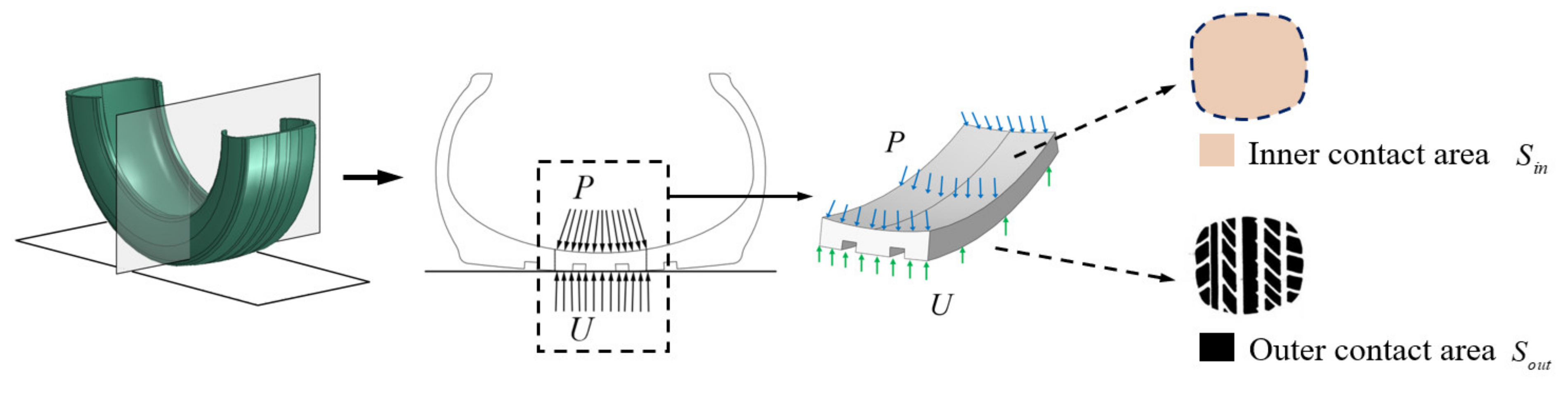
2. Theoretical Analysis of Tire–Road Contact Mechanism

The tire is the only part of the vehicle that contacts the road and the tire–-road interaction is the main source of force generation. Figure 1 shows a model of contact between the tire and the road.

The free-body diagram of the isolated part and the surrounding area of the contact part is shown in Figure 1. Since the deformation of the isolated body is small, the forces on the sides can be ignored. Thus, the equilibrium equation of the isolated body can be expressed as

$$P{S}_{in}=U{S}_{out}$$

(1)

where $S_{in}$ is the inner contact area; $S_{out}$ is the outer contact area; $P$ is the tire inflation pressure; $U$ is the average tire–road contact pressure. The inner contact area is very difficult to measure. Herein, it is assumed that the inner contact area and the outer contact area have the same shape. However, due to the longitudinal and lateral grooves in the tire tread, the value of $S_{out}$ is not equal to $S_{in}$. In terms of Equation (1), the tire–road contact force can be acquired in two ways, that is, by multiplying the inner contact area with the tire inflation pressure, or multiplying the outer contact area with the average contact pressure. This study focuses on the former method as elaborated below and the inner contact area is simply referred to as the contact area.

In most cases, researchers assume that the contact area is a circular or elliptical shape with contact length $a$ and contact width $b$ [29]. The tire geometry is shown in Figure 2.

In terms of the geometric relationship, the contact length $a$ and width $b$ can be expressed by the tire radius $r$ and tire tread radius $R_n$, respectively,

$$\left\{\begin{array}{l}a=2\sqrt{2r\delta -{\delta }^2}\\ b=2\sqrt{2R_n\delta -{\delta }^2}\end{array}\right.$$

(2)

where $\delta$ is the tire vertical deflection. From the tire cross-section in Figure 2b, the tire radius $r$ and the tread radius $R_n$ can be expressed as [30],

$$\left\{\begin{array}{l}r=0.5D+H\\ R_n=0.5h+0.125\frac{B^{\prime }{}^2}{h}\end{array}\right.$$

(3)

where $h$ and $B^{\prime }$ are the height and width of the tread cap, respectively; $H$ is the height of the carcass section, $B$ is the section width; $D$ is the rim diameter. For a specific tire type, the tire section parameters including $B$, $H$, and $D$ can be obtained by referring to the tire design standards [31]. The height $h$ and width $B^{\prime }$ of the tread cap are the main parameters determining the shape of the tire section. Typical design criteria suggest that the ratios of $h/H$ and $B^{\prime }/B$ should be set within a specific range to achieve the best performance of the tire. For example, the ratio $B^{\prime }/B$ is usually set in the range of 0.6–0.9 to avoid an excessive tire-road contact area that affects the service life of the tire. The mean value of 0.75 was assumed for the ratio $B^{\prime }/B$ and the corresponding ratio $h/H$ was taken as 0.03 for the present study in the later sections [30,32,33]. By substituting Equation (3) into Equation (2), the contact length $a$ and width $b$ can be expressed as

$$\left\{\begin{array}{l}a=2\sqrt{(D+2H)\delta -{\delta }^2}\\ b=2\sqrt{(h+0.25\frac{B^{\prime }{}^2}{h})\delta -{\delta }^2}\end{array}\right.$$

(4)

As the actual tire contact area is difficult to estimate, it is usually assumed to be a simple geometry, and the contact length $a$ and width $b$ are important parameters to calculate the contact area. For different tire types, different shapes are assumed for the contact area. The contact area of passenger car tires is usually assumed to be an oval shape [34]. Accordingly, the contact area $S_{Oval}^{}$ is expressed as

$$S_{Oval}^{}=0.25\pi ab$$

(5)

For heavy trucks, the contact area is approximated as a rectangular shape rather than a circular shape and the contact area $S_{Rec}$ is expressed as

$$S_{Rec}=ab$$

(6)

Huang et al. [29] assumed that the contact area of truck tires is a combination of a rectangle with two half circles on each side, and the contact width $b$ is assumed to be $0.6a$, as shown in Figure 3. Thus, the contact area $S_{Com}^{}$ is approximated using the following equation:

$$S_{Com}^{}=\pi {(0.3a)}^2+(0.4a)(0.6a)=0.5227a^2$$

(7)

However, due to the complicated structural composition and material properties of tires, the assumptions of simple geometry are not able to predict the actual contact area during the deformation process. Therefore, a more realistic tire model will be established based on the numerical analysis as follows.

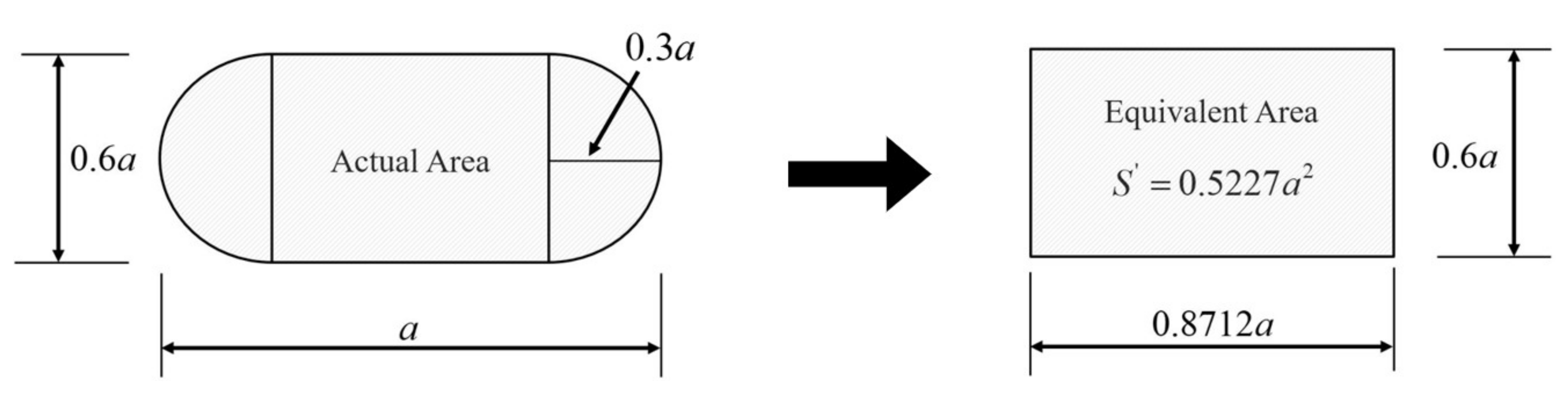
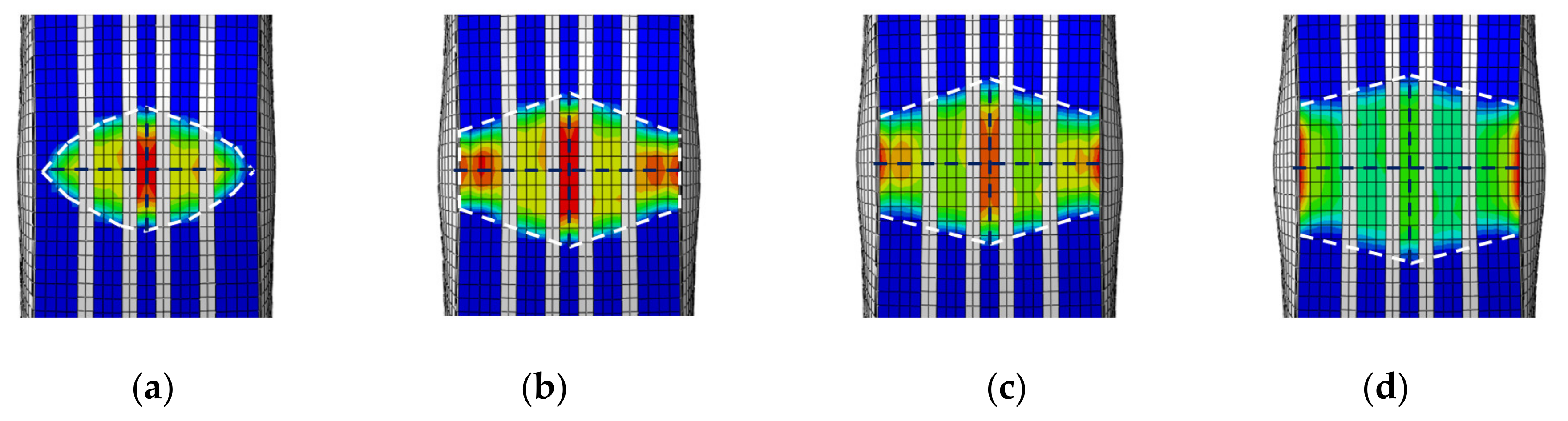
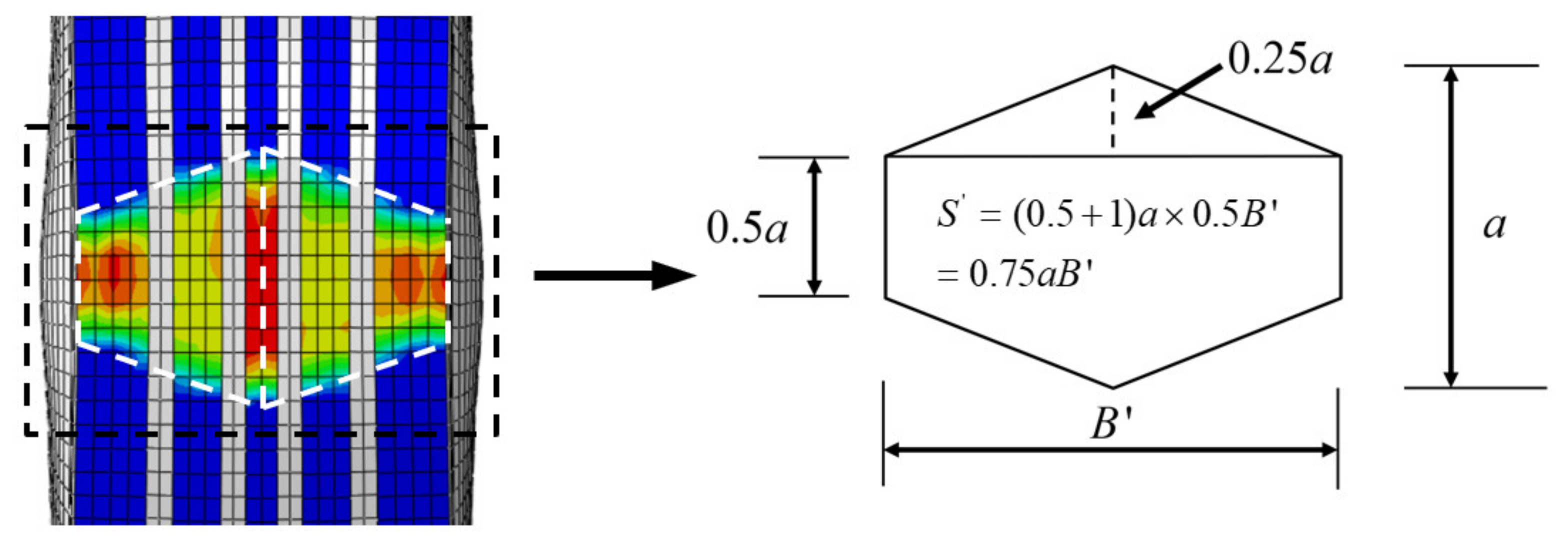
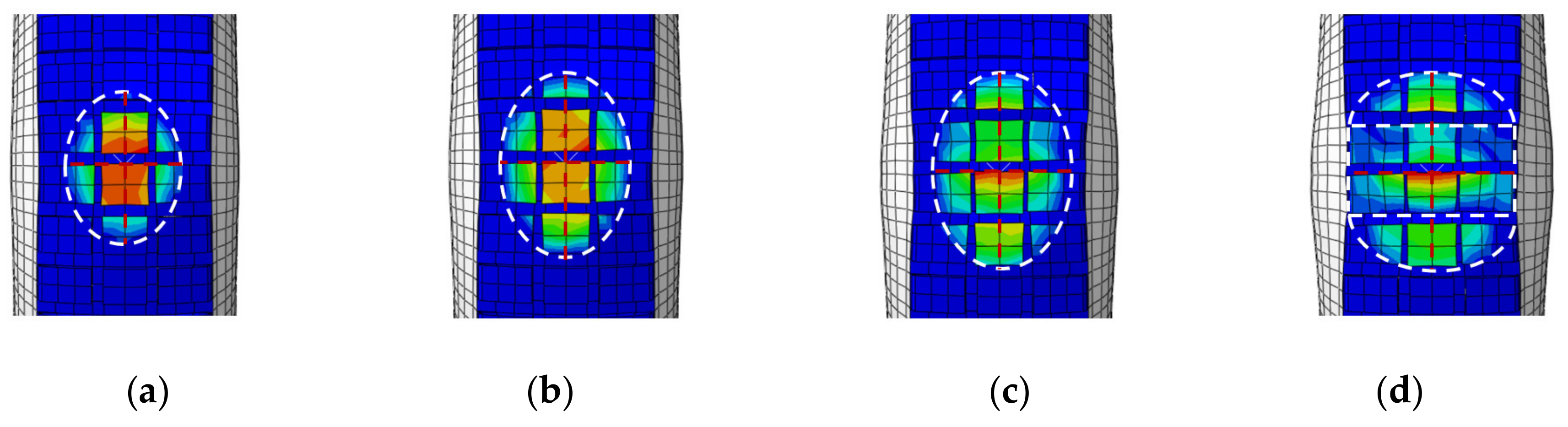
3. Tire–Road Contact Force Equations through Numerical Analysis

In this section, various tires were simulated in ABAQUS and the tire force–deformation equation was established based on the simulation results.

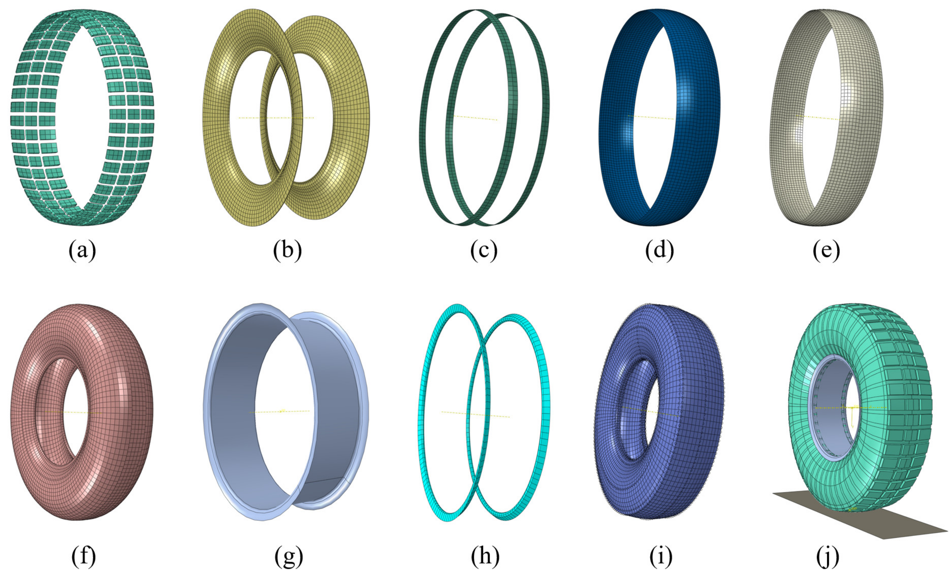
3.1. Establishment of Tire FE Model

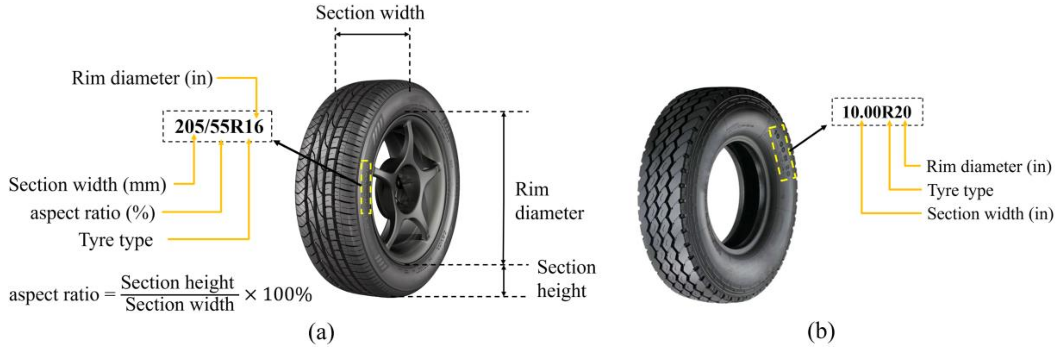
3.1.1. Tire Classification and Selection

According to the tire design standards, tires are categorized in terms of the vehicle type such as the earth-mover, agricultural vehicle, truck, passenger car, and industrial vehicle [31,35,36,37,38]. The present study focused on the tires of trucks and passenger cars, as shown in Figure 4. The tire specification can be identified through the tire sidewall markings that are required to be printed at the time of production, including the tire section width, aspect ratio, type, rim diameter, etc. [39]. Some commonly used tire specifications are listed in

Table 1. Specifications of tire.

Vehicle Type	Tire Specification
Passenger Car	195/55R16	205/55R16
	225/55R16	225/60R18
	235/65R18	245/60R17
Truck	8.00R20	9.00R20
	10.00R20	11.00R20
	11.00R22	12.00R20

.

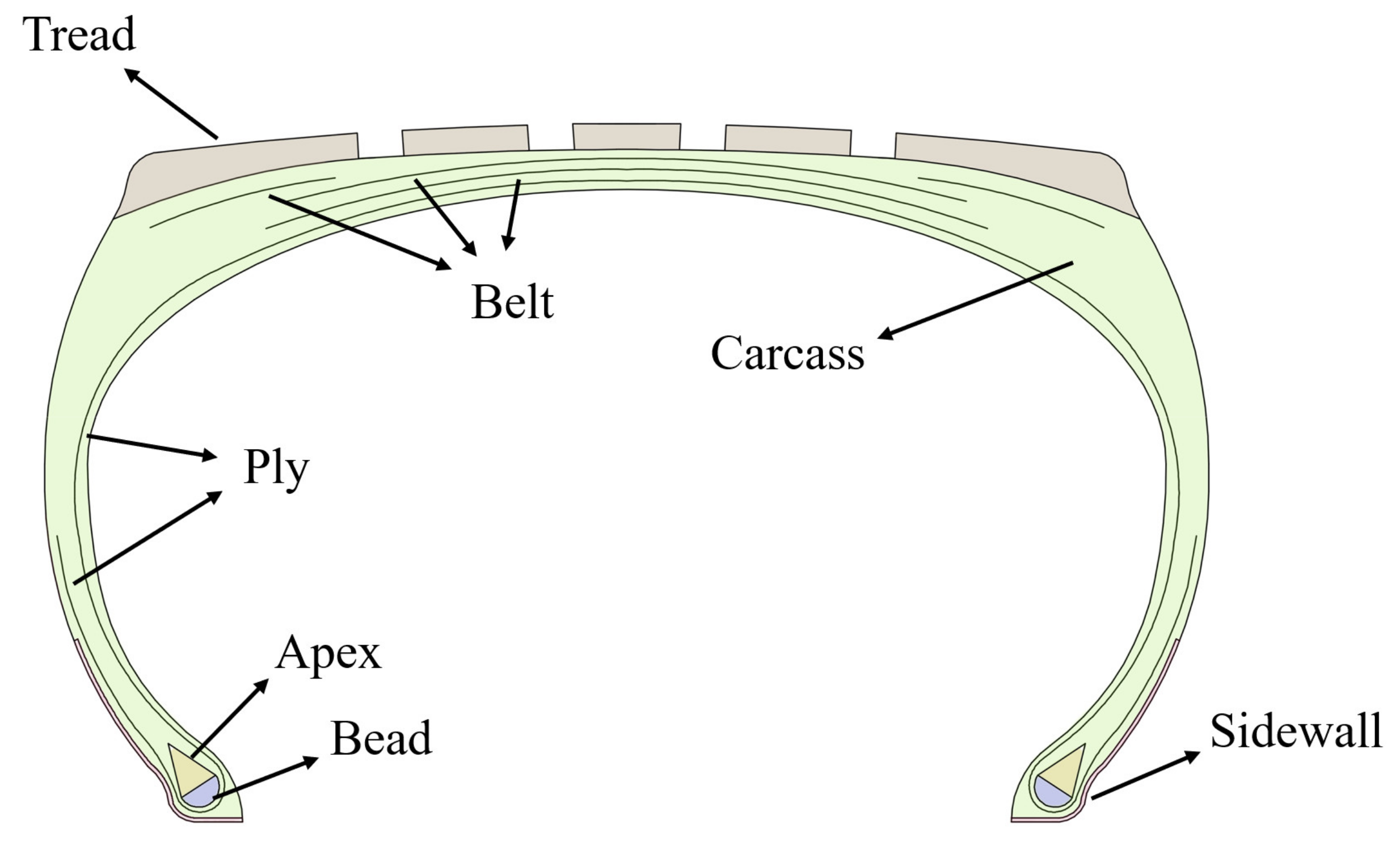
3.1.2. Tire Section and Material

The 11.00R20 truck tire was taken as an example to demonstrate the tire modeling process. The radial tire is mainly composed of the tread, belt, carcass, bead, sidewall, apex, ply, and other parts, as shown in Figure 5. The Yeoh material model was chosen for simulating the tire rubber according to its uniaxial tensile test results [27]. Unlike the isotropic rubber material, the ply and belt of the tire are composite structures with anisotropy properties. The rebar reinforcement layer was selected to simulate the tire’s reinforced skeleton structure. The parameters of the Yeoh model and rebar model are referred to in the literature [40].

D Tire Model

The 3D geometric model of the tire was generated through rotating the tire section shown in Figure 5 by 360° about the central axis, and different material properties were assigned to the corresponding parts. The total number of cells and nodes were 185,710 and 214,070, respectively. The rubber used the eight-node linear hexahedron element (C3D8R), and the skeleton structure used the four-node quadrilateral membrane element (M3D4R). The tire inflation pressure was realized by exerting pressure on the inner surface of the tire. The rim and the road were regarded as rigid bodies without deformation. The surface-to-surface contact type was used between the tire and the road, and binding constraints were adopted between the tire and the rim. The FE model of the truck tire in ABAQUS is shown in Figure 6. The modeling process of the passenger car tire is similar and not elaborated here.

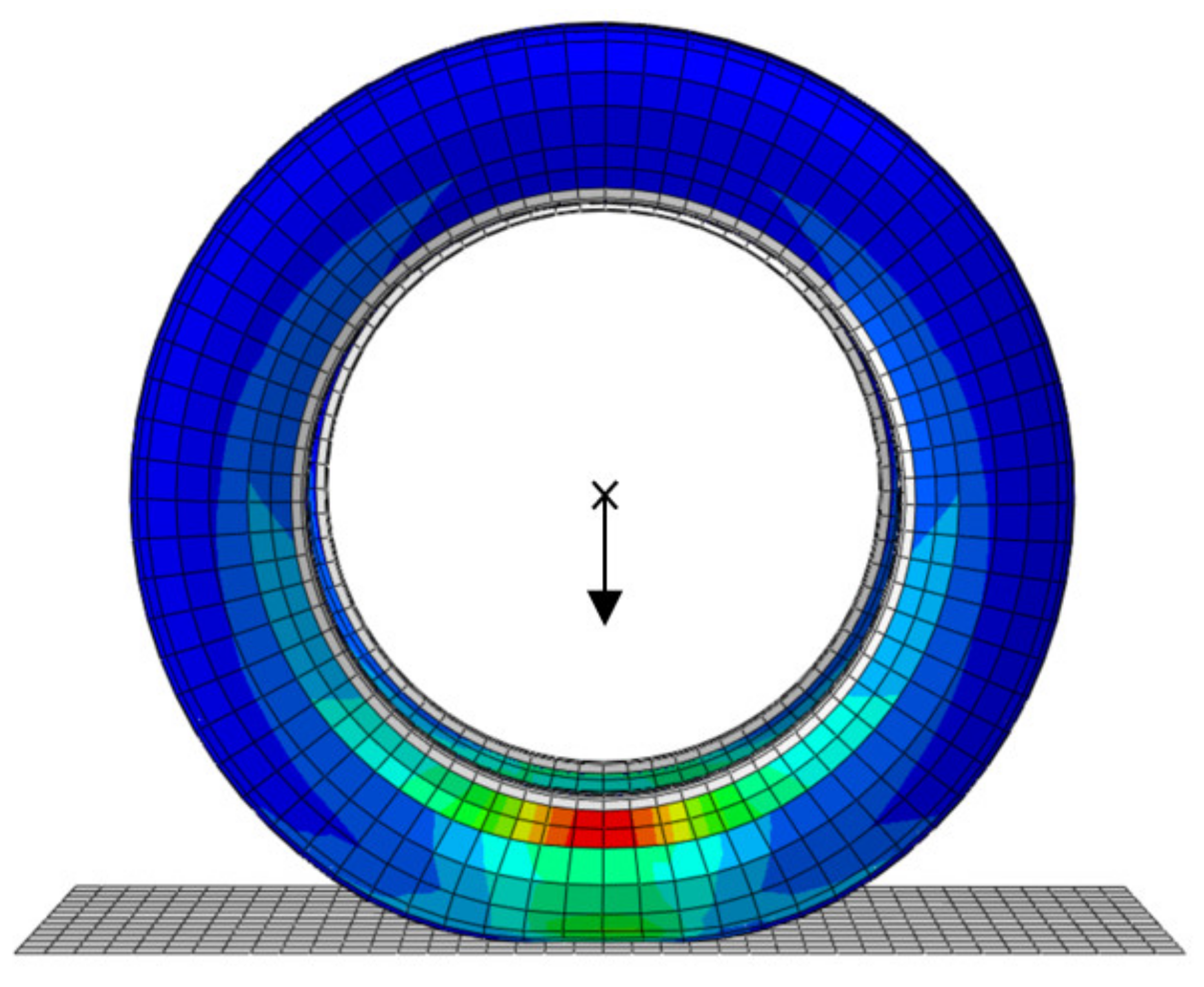
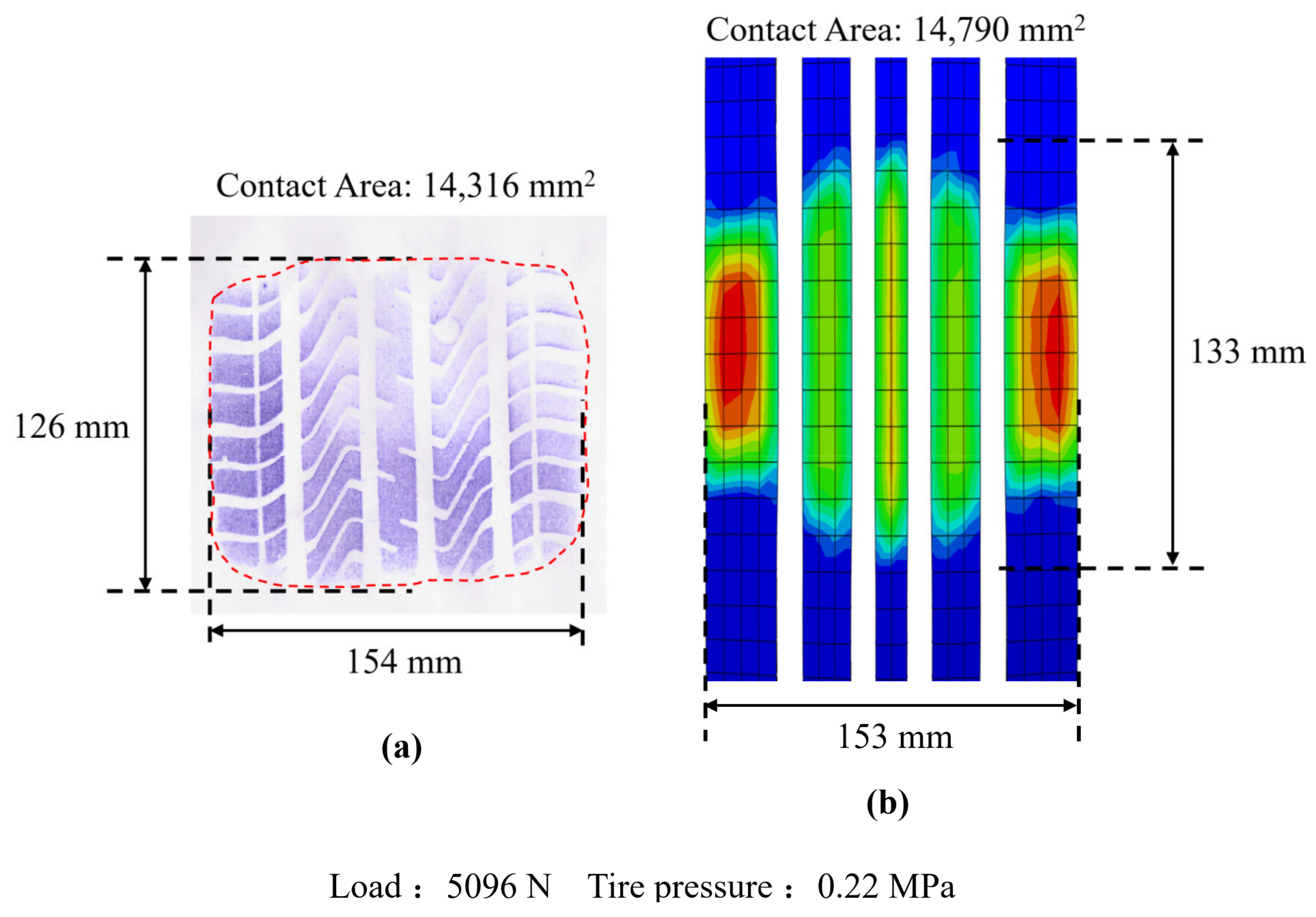
3.2. Verification of Tire FE Model

The static analysis was conducted on the tire model. The center point of the rim was set as the reference point and the concentrated force was applied on it as shown in Figure 7.

To evaluate the performance of the FE model, the tire footprint was compared with the experiment result. Figure 8 shows the field test used to obtain the tire footprint through the copying paper placed at the bottom of the tire.

The dimensions of the obtained footprint were measured in MATLAB. The contact length is 126 mm; the contact width is 154 mm; the contact area (outer edge excluding the strip grooves) is 14,316 mm². Meanwhile, the footprint from the FE model was also obtained as shown in Figure 9.

Table 2. Comparison of the tire footprint.

	Contact Length	Contact Width	Contact Area
Simulation results	133 mm	153 mm	14,790 mm
Measured results	126 mm	154 mm	14,316 mm
Absolute error (AE)	5.2%	0.6%	3.3%

presents the comparison results of the footprints. The values of the contact length, contact width, and contact area are in good agreement between the simulation and measured results, and the maximum error is 5.2%, which verifies that the FE model performs well in simulating the actual tire.

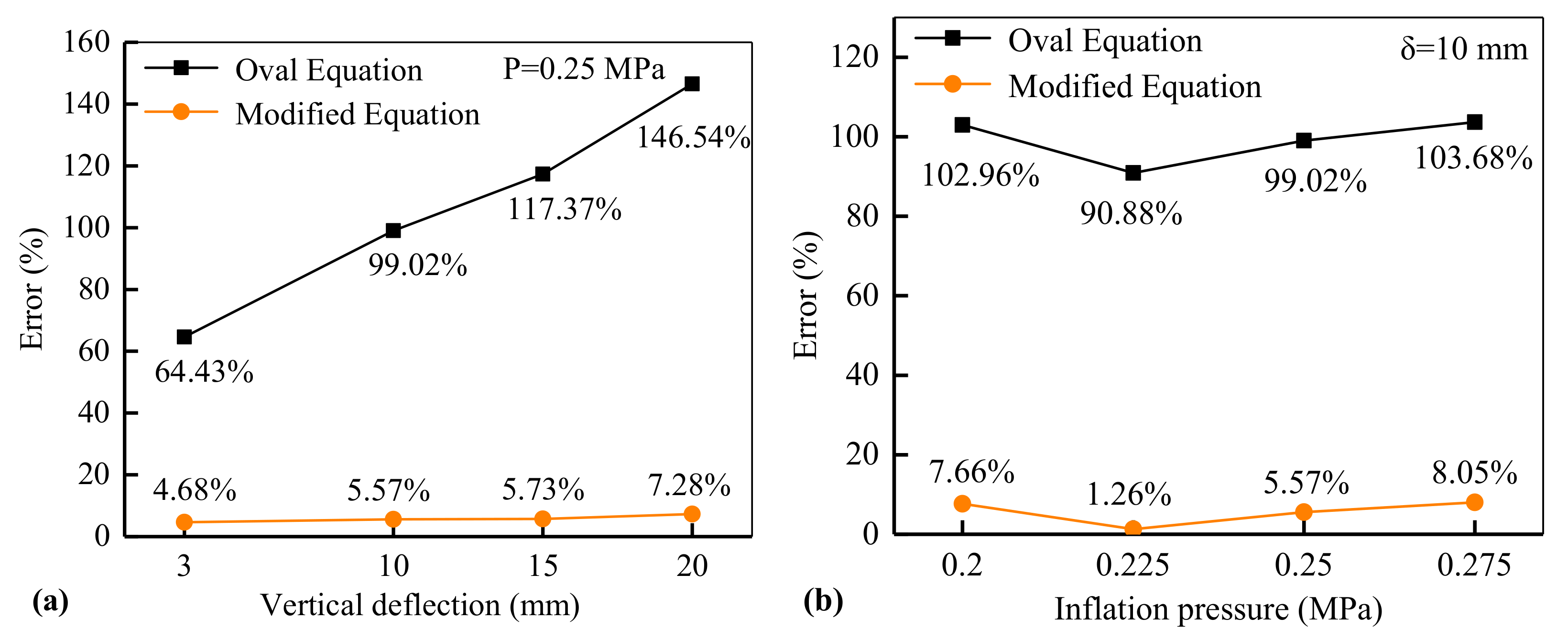
3.3. Tire Contact Force Equations

The verified tire FE models (205/50R16 passenger car tire and 11.00R20 truck tire) were analyzed under different conditions. For the passenger car tire, the following cases were analyzed: tire inflation pressure of 0.2, 0.225, 0.25, and 0.275 MPa, and vertical deflection of 3, 10, 15, and 20 mm.

The tire footprints under different vertical deflections were extracted as shown in Figure 10. It can be seen that under constant inflation pressure, the area of the tire footprint increases with the increase in tire deflection. When the vertical deflection is small and the contact width is smaller than the tread width, the footprint edge looks like a rhombus, as shown in Figure 10a. As the vertical deflection increases, the contact width reaches the tread width, and thereafter the footprint keeps increasing along the longitudinal direction. The footprint edge becomes a hexagon, as shown in Figure 10b and Figure 11d. In addition, under the constant vertical deflection, the footprint under different inflation pressure is almost the same. This implies that the footprint shape is mainly affected by the vertical deflection.

In terms of the above simulation results, the footprint of passenger car tire is not always an oval shape as assumed in Equation (5). It is actually a rhombus when the contact width is smaller than the tread width, and a hexagon when the contact width is larger than the tread width. Based on the analysis of multiple sets of simulation results, the length of the hexagon edge is about half the contact length, thus it is assumed to be $0.5a$, as shown in Figure 11.

Accordingly, Equation (5) can be modified as

$$S_{Car}=\left\{\begin{array}{cc}2\delta \sqrt{D+2H-\delta }\sqrt{h+0.25\frac{B^{\prime }{}^2}{h}-\delta }\hfill & , b<B^{\prime }\hfill \\ 1.5B^{\prime }\sqrt{(D+2H)\delta -{\delta }^2}\hfill & , b=B^{\prime }\hfill \end{array}\right.$$

(8)

By substituting Equation (8) into Equation (1), the tire–road contact force of the passenger car tire can be expressed as

$$F_{Car}=\left\{\begin{array}{cc}2P\delta \sqrt{D+2H-\delta }\sqrt{h+0.25\frac{B^{\prime }{}^2}{h}-\delta }\hfill & , b<B^{\prime }\hfill \\ 1.5P{B}^{\prime }\sqrt{(D+2H)\delta -{\delta }^2}\hfill & , b=B^{\prime }\hfill \end{array}\right.$$

(9)

The calculated results of the tire contact force under different area assumptions are shown in

Table 3. Contact forces of passenger car tire.

Tire Type	Inflation Pressure (MPa)	Vertical Deflection (mm)	Simulation Force (N)	Oval Equation (N)	Modified Equation (N)
205/50R16	0.25	3	1549.5	2547.9	1622.0
	0.25	10	4235.1	8428.5	4471.2
	0.25	15	5784.6	12,573.6	5453.3
	0.25	20	6762.7	16,672.6	6270.5
	0.2	10	3322.3	6742.8	3576.9
	0.225	10	3974.1	7585.6	4024.1
	0.275	10	4552.0	9271.3	4918.3

.

The relative error (RE) is used to evaluate the accuracy of the contact force estimation as

$$e_{RE}=\left|\frac{F_{Eq}-F_{FEA}}{F_{FEA}}\right|\times 100\%$$

(10)

where $F_{Eq}$ is the “calculated force”; and $F_{FEA}$ is the “simulation force”. The comparison of the error results is shown in Figure 12.

Figure 12a represents the relative error of the contact force under different vertical deflections with an inflation pressure of 0.25 MPa. It is seen that the contact force estimated by the oval equation (i.e., Equation (5)) is much larger than the simulation results, and the error increases with the increase in tire vertical deflection, with a maximum error of 146.54%. Although the error of the modified equation (i.e., Equation (9)) also increases during the vertical deflection from 3 mm to 20 mm, it is in the range of 4.68~7.28%. Figure 12b represents the relative error under different inflation pressure with constant vertical deflection. The error of the oval equation is about 100%. In contrast, the modified equation yields satisfactory results and the maximum error is 8.05%. The results indicate that the contact forces estimated by the equation based on the oval assumption have a large difference from the simulation results. On the contrary, the equation based on the modified footprint achieved excellent results in the calculation of tire force.

Compared to passenger car tires, truck tires always have higher inflation pressure and load. Meanwhile, the deformation process of truck tires is also different from that of passenger car tires. It is noted that based on the statistical analysis of the measured data, the actual inflation pressure of the truck generally exceeds the standard inflation pressure [41]. Thus, the inflation pressure of the truck tire was set in the range of 0.7 MPa to 1 MPa, and the vertical deflection was in the range of 10 mm to 20 mm. Figure 13 shows the footprint results of a truck tire under different vertical deflections.

As for the truck tire with heavy load, the tire contact length is usually larger than the contact width. In Figure 13a–c, as the deformation of the tire is small, the contact width is smaller than the tread width and the shape of the footprint looks like an oval. Referring to the assumption in Section 2, the contact width $b$ of the truck tire is assumed to be $0.6a$. Similarly, when the contact width is equal to the tread width as shown in Figure 13d, the footprint is likely to be a combination of a rectangle with two half circles on each side, which is the same as the assumption in Section 2. Accordingly, the improved contact force equation of truck tires can be expressed as:

$$S_{Truck}=\left\{\begin{array}{cc}0.6\pi \delta (D+2H-\delta )\hfill & , b<B^{\prime }\hfill \\ B^{\prime }[2\sqrt{(D+2H)\delta -{\delta }^2}-(1-0.25\pi )B^{\prime }]\hfill & , b=B^{\prime }\hfill \end{array}\right.$$

(11)

By substituting Equation (11) into Equation (1), the tire–road contact force of the passenger car tire can be expressed as

$$F_{Truck}=\left\{\begin{array}{cc}0.6\pi P\delta (D+2H-\delta )\hfill & , b<B^{\prime }\hfill \\ P{B}^{\prime }[2\sqrt{(D+2H)\delta -{\delta }^2}-(1-0.25\pi )B^{\prime }]\hfill & , b=B^{\prime }\hfill \end{array}\right.$$

(12)

The calculated results for the tire–contact force under different footprint assumptions are shown in

Table 4. Contact forces of truck tire.

Tire Type	Inflation Pressure (MPa)	Vertical Deflection (mm)	Simulation Force (N)	Rectangular Equation (N)	Huang Equation (N)	Modified Equation (N)
11.00R20	0.8	10	14,758.4	37,623.7	17,676.5	15,936.2
	0.8	15	23,037.7	56,194.2	26,389.2	23,791.1
	0.8	20	31,357.9	74,603.8	35,018.4	31,570.7
	0.8	25	38,156.4	92,852.4	43,563.9	39,274.9
	0.7	20	26,268.3	65,278.3	30,641.1	27,624.4
	0.9	20	34,197.8	83,929.3	39,395.7	35,517.1
	1	20	36,414.2	93,254.7	43,773.0	39,463.4

.

The relative errors are shown in Figure 14. It should be noted that the values calculated by the rectangular equation (i.e., Equation (6)) in Table 4 are much larger than the simulation value. Thus, the error of the rectangular equation is not analyzed in the figure.

From Figure 14a,b, we can see that the change trend in the Huang equation (i.e., Equation (7)) and the modified equation (i.e., Equation (12)) is similar. Meanwhile, the force estimation error is smaller compared with that of the passenger car. The error of the Huang equation is in the range of 11.67~20.21% while the error of the modified equation is in the range of 0.68~8.37%. This means that the footprint-modified equation significantly improves the results.

According to the analysis in this section, the traditional footprint assumptions are not reasonable; thus, the tire force equation has a large error in the calculation of tire force. Actually, the footprint approximates different shapes at different deformation stages of tires. FE models of different tires were established to analyze the deformation process of the tire. The simulation results show that the tire footprint approximates different shapes at different deformation stages. For passenger cars, the tire footprint is not always an oval shape as assumed. It is actually a rhombus when the contact width is smaller than the tread width, and a hexagon when the contact width reaches the tread width. As for the tires of heavy trucks, the footprint is an oval when the contact width is smaller than the tread width, and a rectangle with two half circles on each side when the contact width reaches the tread width. The equation based on the modified footprint achieves better results, and the errors are all within 10%.

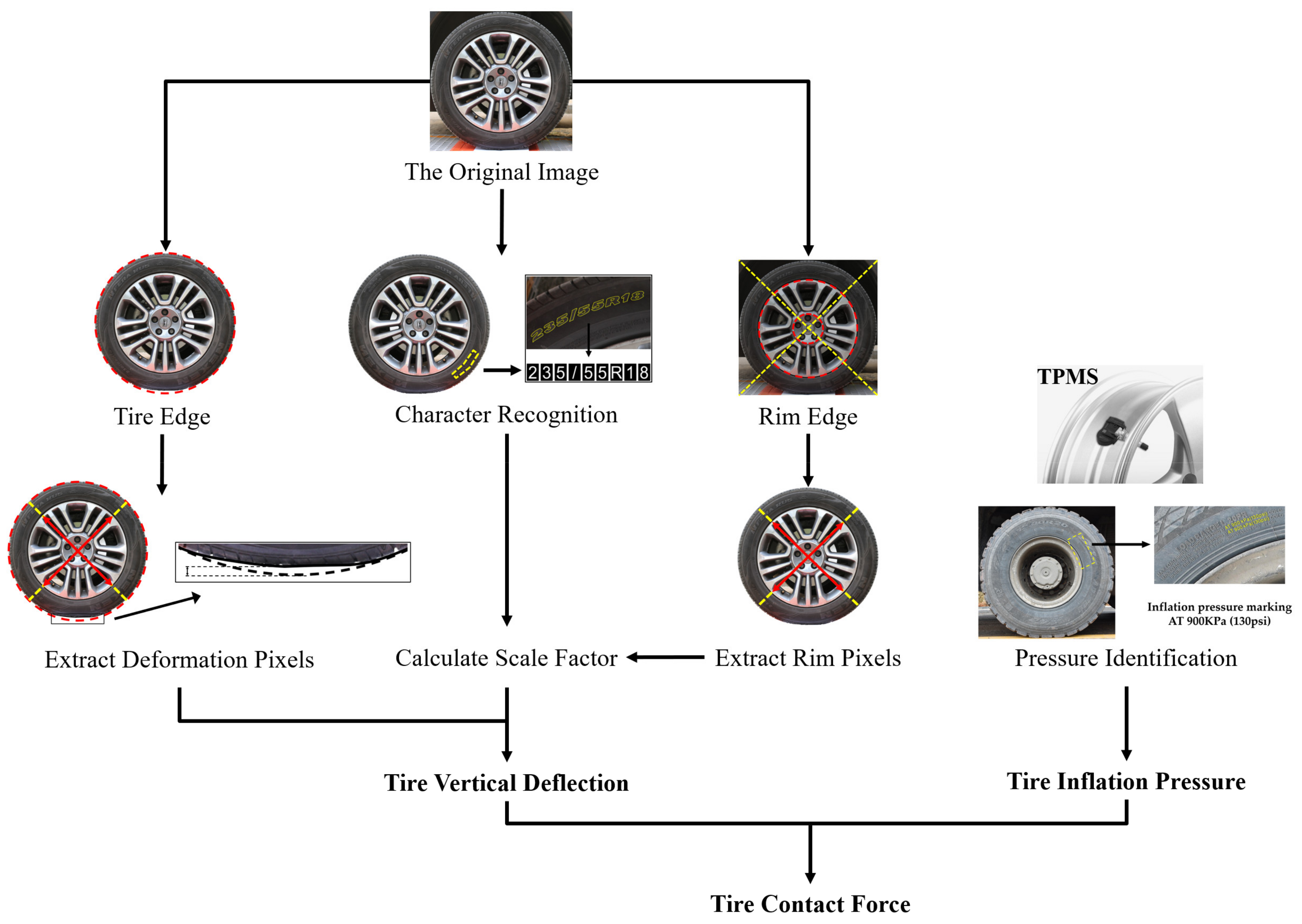
4. Methodology of Vision-Based Vehicle Weight Identification

In the previous sections, the equations of tire–road contact force were established. In terms of the equations, the tire–road contact force could be estimated as long as the tire inflation pressure, tire vertical deflection, and other physical parameters are known. The vehicle weight can then be identified by summing the contact forces of all the tires as,

$$G={\displaystyle \sum _1^i{F}_i}={\displaystyle \sum _1^i{P}_i}{S}_i$$

(13)

where $G$ is the gross weight of the vehicle; $i$ is the total number of tires; $F_i$ is the contact force of each tire; $P_i$ is the inflation pressure of each tire; $S_i$ is the contact area of each tire. The modified equations of the footprint for passenger car tires and truck tires refer to Equations (9) and (12), respectively.

The main parameters to be measured for the contact force estimation include the inflation pressure $P$, vertical deflection $\delta$, and tire specification parameters such as $D$, $H$, $B$. The authors proposed a computer vision-based method to measure those parameters. A single-lens reflex (SLR) camera is used to capture images of each tire. Then, the computer vision techniques such as the edge detection and character recognition algorithms are used to detect the edges of the tire and rim, tire vertical deflection, and tire sidewall markings from the images, as shown in Figure 15. More details can be found in Kong et al. [28].

For the captured images of the tire, the K-means clustering algorithm [42] is first used for coarse segmentation, and then the region growing segmentation algorithm (RGSA) [43] is applied for fine segmentation. Thus, a continuous, and complete tire edge can be detected from the image background. Then, the Otsu algorithm [44] and projection algorithm [45] are applied for character detection and positioning in the tire sidewall, and the window scanning algorithm is used for character segmentation. After that, the tire specification label can be identified by the template matching algorithm, for instance, 235/55R18, as shown in Figure 15. That is, the section width is 235 mm, the aspect ratio is 0.55, and the rim diameter is 18 in. Since it is reasonable to assume that the rim is rigid, the scale factor of the tire image could be calculated based on the physical value and the pixel number of the rim diameter. The tire vertical deflection can then be calculated by multiplying the scale factor with the pixel number of the vertical deformation, which is the movement of the lowest point of the tire edge before and after the deformation.

The inflation pressure can be measured remotely by pressure sensors, such as the Tire Pressure Monitor System (TPMS) equipped on most vehicles. For vehicles that do not have TPMS, such as most trucks, a computer vision-based method was proposed. Generally, the label on the tire sidewall shows the manufacturer-recommended inflation pressure value, as shown in Figure 16. Based on the statistical analysis of a large set of measured data, the ratio of the measured pressure to the manufacturer-recommended pressure is within a limited range. For heavy trucks, the ratio is in the range of 1.1–1.2 [28]. Herein, a ratio of 1.15 is assumed for a heavy truck. Thus, the inflation pressure can be estimated by multiplying the manufacturer-recommended pressure with the ratio. For example, the inflation pressure of the tire in Figure 16 is equal to 900 × 1.15 = 1035 KPa.

Once the tire vertical deflection, inflation pressure, and specification parameters are obtained, the derived contact force equations are adopted to calculate the contact force of each tire. Finally, the vehicle weight including the axle weight and gross weight can be estimated by summing the contact forces of all the tires.

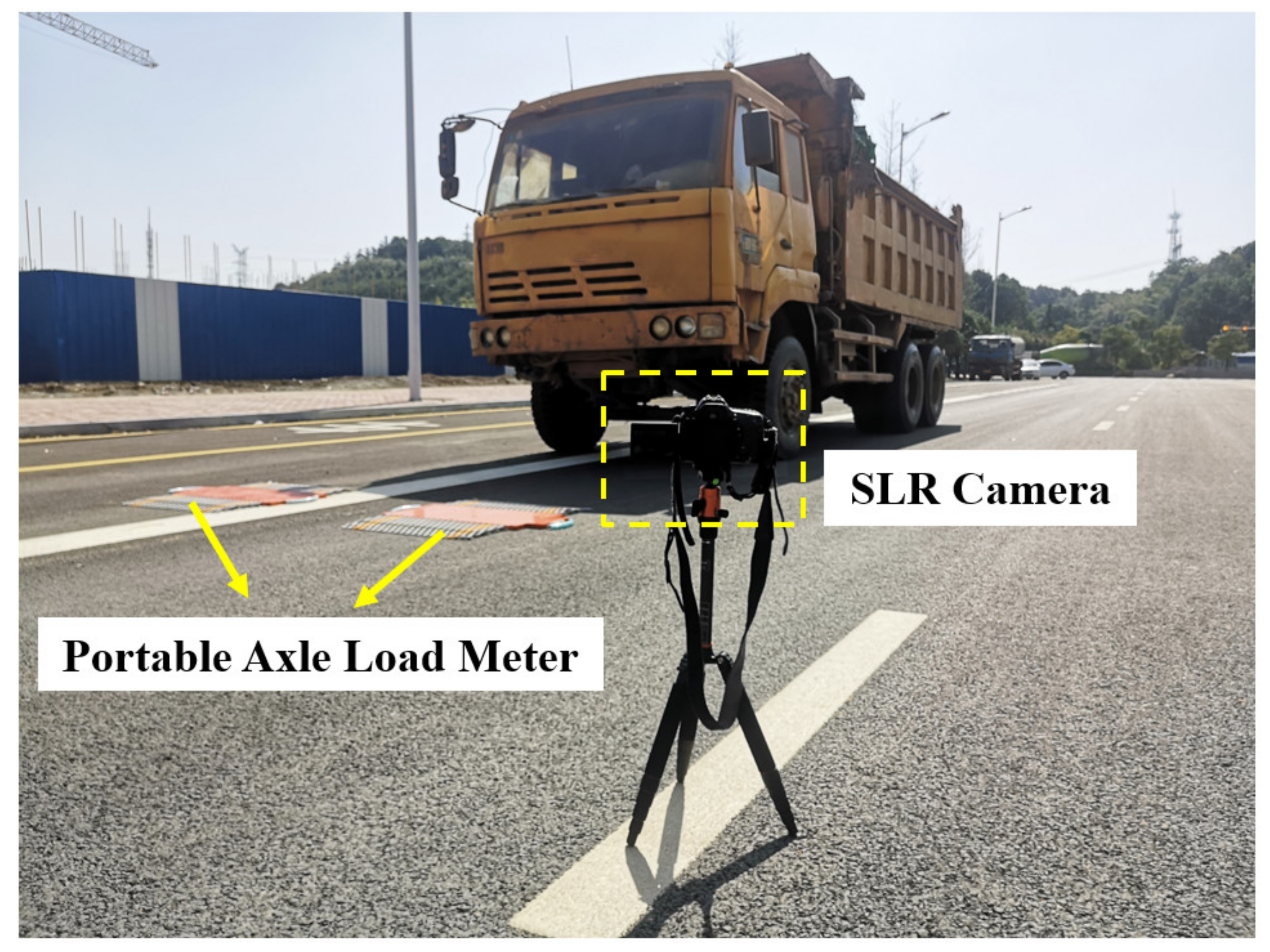
5. Experimental Validation

The purpose of the experiment was to validate the performance of the derived contact force equations, as well as verify the feasibility of the developed vision-based vehicle weight identification method. The experiment was conducted on two 2-axle passenger cars and two 3-axle trucks. As shown in Figure 17, the experimental devices include the portable wireless axle weigh pad, SLR camera, and tire pressure detector. For convenience, the tires are represented as the right front (RF), left front (LF), right middle (RM), left middle (LM), right rear (RR), and left rear (RR) according to their position on the vehicle. The process is described below:

(1)

Actual weight measurement: the portable wireless axle weigh pad was used to measure the stationary axle weight and gross weight of the vehicle. It should be noted that the vehicles were all controlled by the same driver to eliminate the influence of the driver’s weight.

(2)

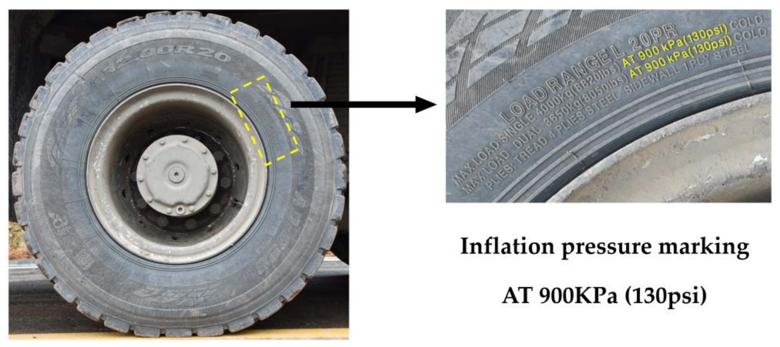
Actual inflation pressure measurement: since most trucks do not have a TMPS, the actual inflation pressure of each truck tire was measured by the pressure detector, which was also used to calibrate the pressure identified using the computer vision method mentioned in Section 4.

(3)

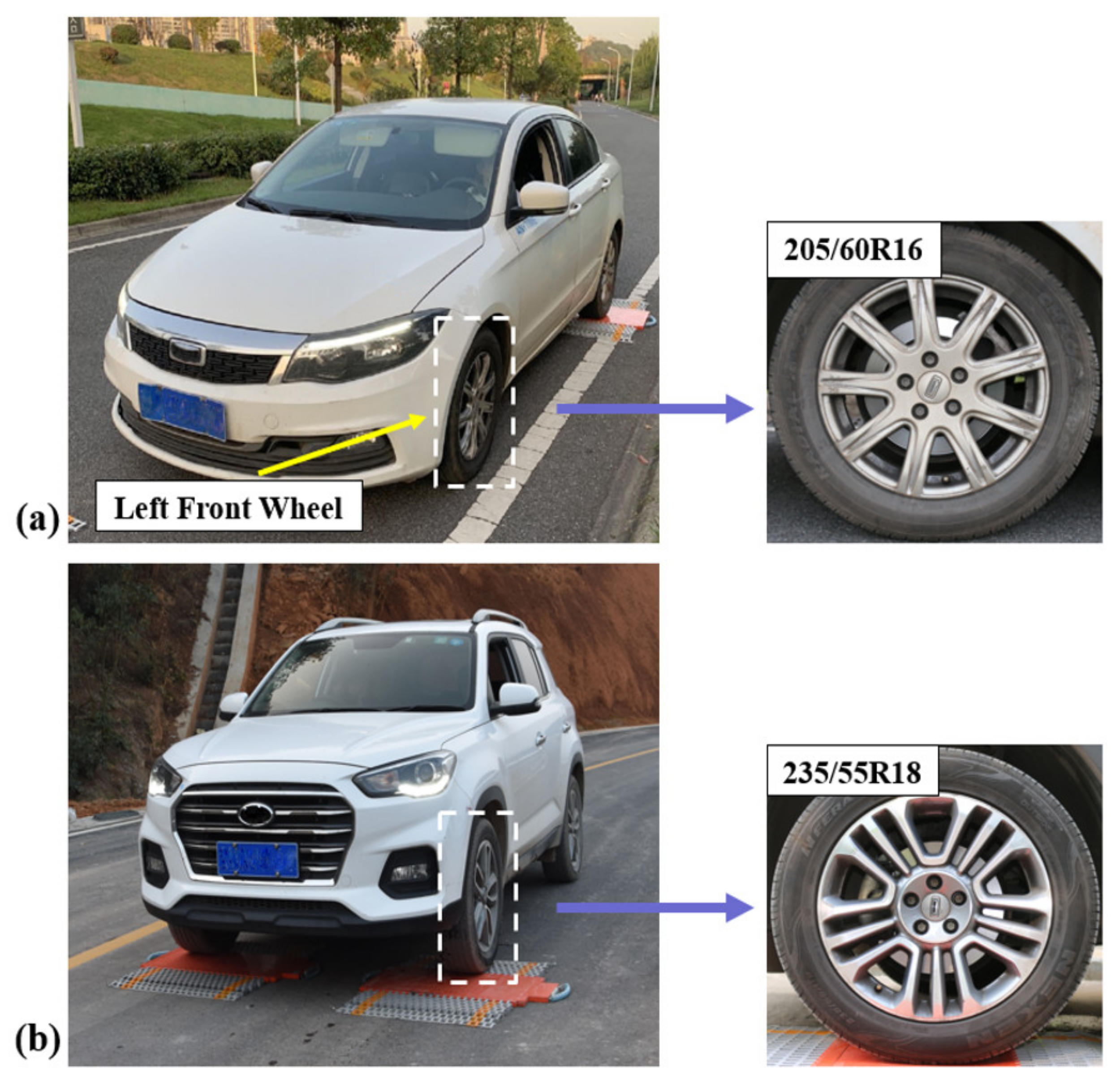
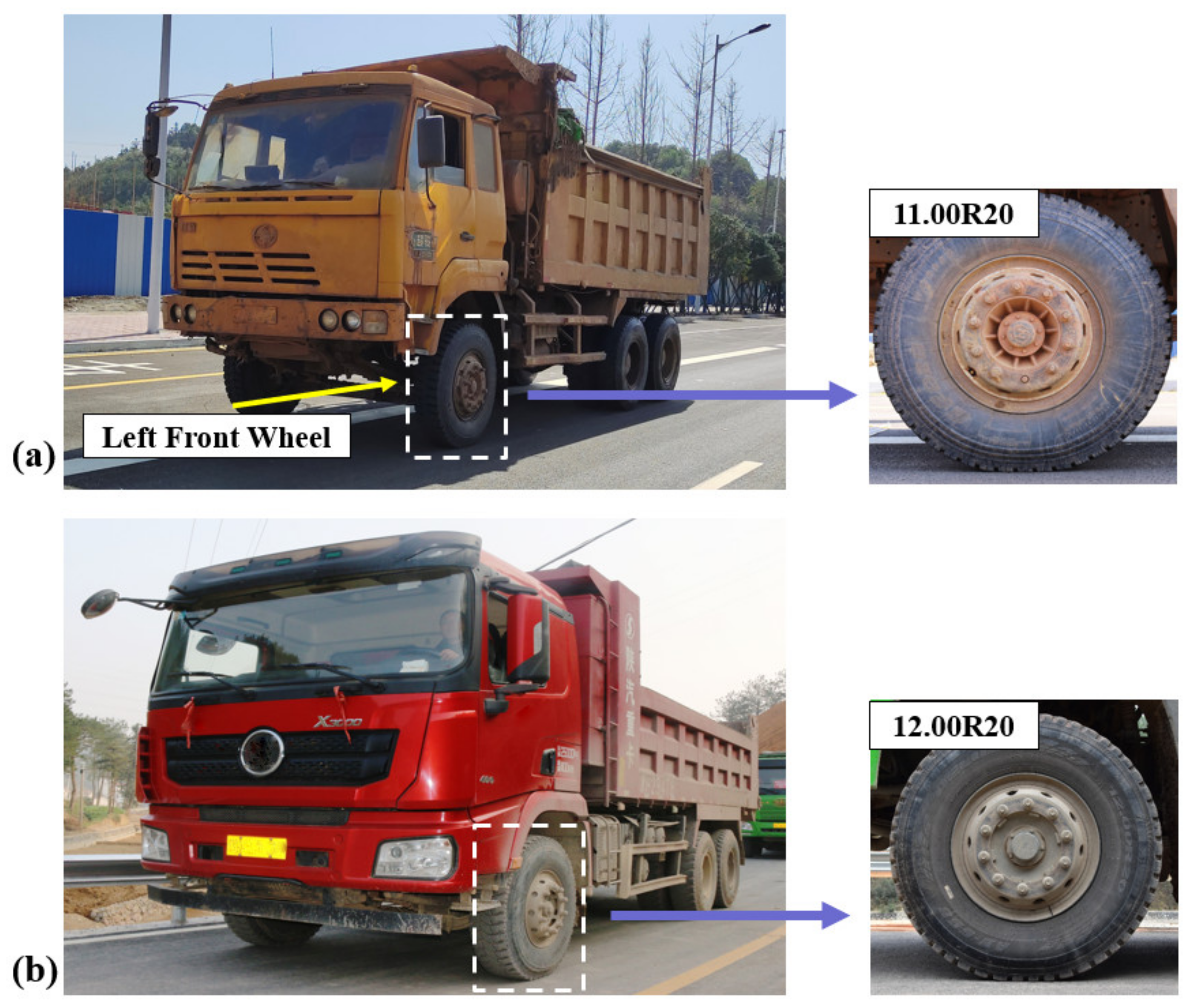
Image acquisition: the tested vehicles traveled on the road at a speed of approximately 15 km/h. The camera was set up on the roadside 5–7 m away from the vehicle and the optical axis was configured as perpendicular to the vehicle traveling direction. Tire images with a resolution of 6000 × 4000 pixels were captured.

(4)

Results and evaluation: the proposed CV-based method was used to calculate the tire contact force in each tire. The absolute error was used to evaluate the accuracy of the weight estimates

$$e_{AE}=\frac{\left|W_I-W_A\right|}{W_A}\times 100\%$$

(14)

where $W_I$ is the identified weight; and $W_A$ is the actual weight.

Figure 17. Field experiment.

Figure 17. Field experiment.

5.1. Weight Identification of Passenger Cars

The tested passenger cars include a sedan with 205/60R16 tires and an SUV with 235/55R18 tires, as shown in Figure 18. Both cars have a TPMS.

The inflation pressure and vertical deflection of each tire, and the actual weight of each axle were measured as shown in

Table 5. Axle weight identification results for passenger cars.

Type	Position	Inflation Pressure (MPa)	Vertical Deflection (mm)	Actual Weight (N)	Oval Equation		Modified Equation
					Calculated Weight (N)	Error	Calculated Weight (N)	Error
Sedan	LF	0.22	16.6	9310	20,584	121.1%	9624	3.3%
	RF	0.2	14.3
	LR	0.19	10.8	6321	12,034	90.4%	6812	7.7%
	RR	0.17	10.2
SUV	LF	0.2	13.6	9996	20,339	103.5%	10,646	6.5%
	RF	0.22	12.5
	LR	0.18	10.6	8134	14,348	76.4%	8723	7.2%
	RR	0.2	9.7

. The axle weights estimated by the oval equation (i.e., Equation (5)) and the modified equation (i.e., Equation (9)) are also shown in the table together with the relative errors. It can be seen that the weights estimated by the oval equation are much larger than the actual weights, with an error of 76.4~121.1%, while the weights estimated by the modified equation are very close to the actual weight, with the error of 3.3~7.7%. This indicates that the accuracy of the modified equation is significantly improved.

In addition, it is observed that the errors in the rear axle weights calculated by the modified equation are slightly larger those in the front axle. Since the sedan and SUV are equipped with the engine at the front, the vertical deflections and axle weights of the front axle were more significant than that of the rear axle, which might be the reason for the differences in the results between the front axle and the rear axle. The gross weights of the sedan and SUV were summed as shown in

Table 6. Gross weight identification results for passenger cars.

Type	Actual Weight (N)	Oval Equation		Modified Equation (N)
		Calculated Weight (N)	Error	Calculated Weight (N)	Error
Sedan	15,631	32,617	108.6%	16,436	5.1%
SUV	18,130	34,687	91.3%	19,369	6.8%

with the relative error. Similarly, the identification of the gross weight using the modified equation provided satisfactory results.

5.2. Weight Identification of Trucks

One 3-axle truck equipped with 11.00R20 tires and the other with 12.00R20 tires were tested, as shown in Figure 19. For multi-axle trucks, except for the front axle, the other axles usually utilize a dual wheel system (DWS). Herein, it is assumed that the inner tire of the DWS has the same contact force as the outer tire [46,47]. It is noted that the middle and rear axles of the truck are DWSs.

Figure 20 shows the measured and estimated inflation pressure, as well as the errors for each axle. Since most heavy trucks are not equipped with TPMS, the pressure detector was used to measure the inflation pressure of the tested trucks, which is the “Measured Pressure (MP)” in the figure. Meanwhile, the identified manufacturer-recommended inflation pressure value of each tire is 0.83 MPa (11.00R20) and 0.9 MPa (12.00R20), and the pressure estimated by the inflation pressure estimation method is the “Estimated Pressure (EP)” in the figure. The error is the average value of the left and right tires of each axle.

As can be seen in Figure 20, the estimated inflation pressure is 1.03 MPa and 0.95 MPa, and the measured inflation pressure value is in the range of 0.90~1.10 MPa. Most of the errors in the axle identification are within 10%, except for the front axle of the truck with 11.00R20 tires (=11.5%), which is slightly higher. Overall, the estimated value is close to the measured value.

To evaluate the accuracy of the truck weight estimate, the axle and gross weights were identified by the rectangular equation (i.e., Equation (6)), the Huang equation (i.e., Equation (7)), and the modified equation (i.e., Equation (12)), respectively, as shown in

Table 7. Axle weight identification results for trucks.

Specification	Position	Estimated Pressure (MPa)	Deflection (mm)	Actual Weight (N)	Rectangular Equation		Huang Equation		Modified Equation
					Calculated Weight (N)	Error	Calculated Weight (N)	Error	Calculated Weight (N)	Error
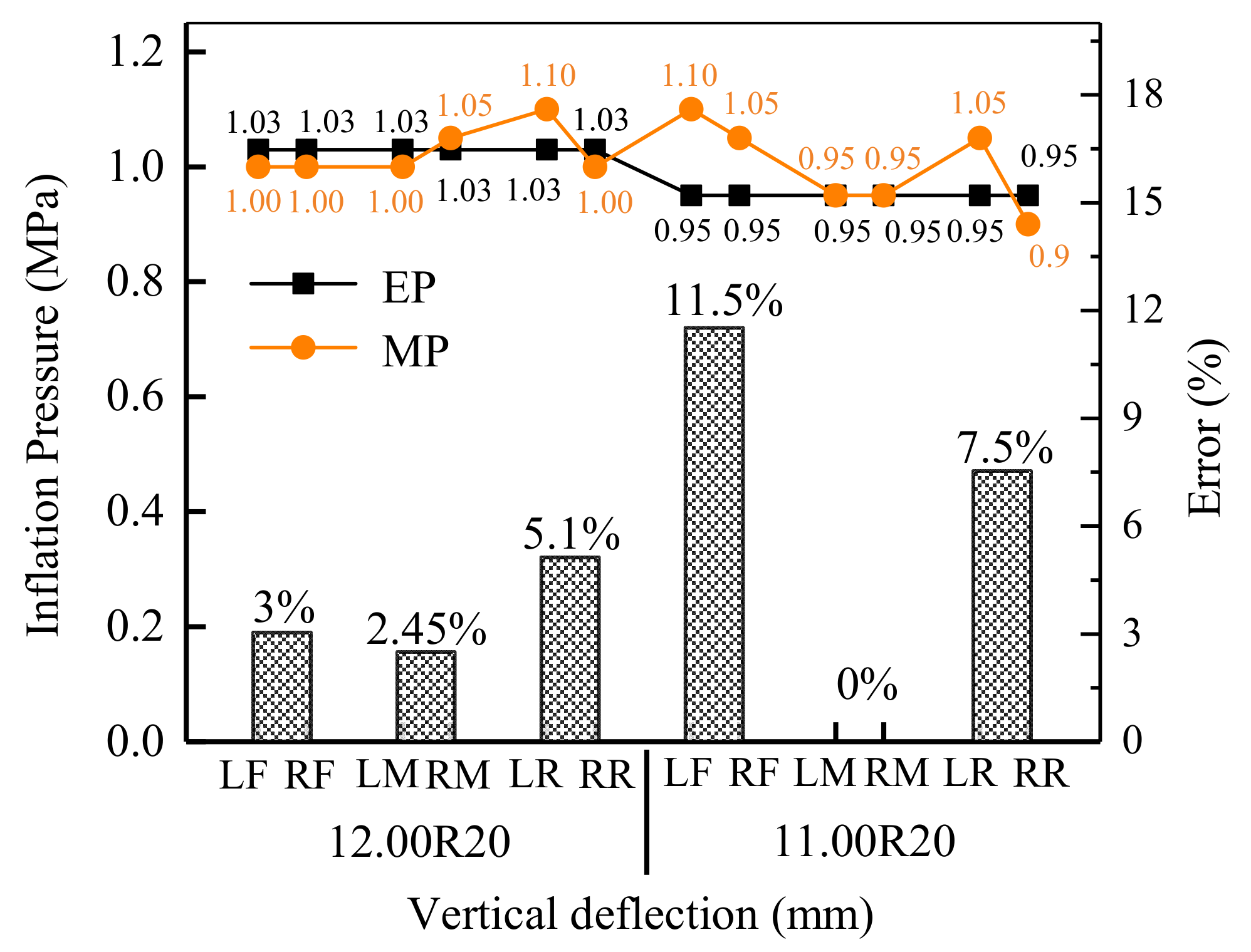
12.00R20	LF	1.03	18.0	77,224	205,052	165.5%	94,299	22.1%	84,642	9.6%
	RF	1.03	21.9
	LM	1.03	20.2	165,228	433,395	162.3%	199,290	20.6%	179,669	8.7%
	RM	1.03	22.0
	LR	1.03	19.6	170,618	432,364	153.4%	198,816	16.5%	179,242	5.1%
	RR	1.03	22.5
11.00R20	LF	0.95	14.1	60,074	133,455	122.2%	62671	4.3%	56,501	6.0%
	RF	0.95	15.9
	LM	0.95	20.5	127,890	326,401	155.2%	153,229	19.8%	138,143	8.0%
	RM	0.95	16.3
	LR	0.95	21.0	136,122	334,253	145.6%	156,908	15.3%	141,460	3.9%
	RR	0.95	16.7

and

Table 8. Gross weight identification results for trucks.

Specification	Actual Weight (N)	Rectangular Equation		Huang Equation		Modified Equation
		Calculated Weight (N)	Error	Calculated Weight (N)	Error	Calculated Weight (N)	Error
12.00R20	413,070	1,070,811	159.2%	492,406	19.2%	443,554	7.4%
11.00R20	324,086	794,109	145.0%	372,809	15.0%	336,105	3.7%

. The actual value of the weight is also listed in Table 7 and Table 8. It is noted that the weight calculation is based on the estimated pressure in Figure 20. It can be seen that the modified equation shows better accuracy with the relative error in the range of 3.7~9.6%, while on the contrary, the rectangular equation and the Huang equation have a larger error of around 150% and 20%, respectively.

In addition, it is noted that the establishment of the theoretical equation was based on the ideal tire structure without consideration of the tire loss. In this test, some truck tires are in a relatively poor condition, as displayed in Figure 21, which might increase the identification error. The tire loss could be a critical issue that needs to be studied in the future.

5.3. Remarks

Based on the proposed vehicle weight identification method discussed in Section 4, the weights of two 2-axle passenger cars and two 3-axle trucks were identified in the field test. Four tire force equations based on different footprint assumptions were compared. The results show that the proposed vision-based vehicle weight identification method can effectively identify the axle weight and gross weight of the vehicle. The identification error of the axle weights and gross weights are both within 10%, regardless of passenger car tires or truck tires. In contrast, traditional footprint assumptions, such as oval, rectangular, and Huang’s assumption are not accurate; therefore, the tire contact force equations have large errors. For the oval equation and rectangular equation, the errors in the axle and gross weight identification are all greater than 50%, and the errors for the Huang equation are about 20%. Thus, the equations based on the modified footprint are a significant improvement in vehicle weight estimation.

6. Conclusions

In this study, the tire–road contact mechanism was studied theoretically, and numerical analyses were conducted to develop the tire contact force equations. The methodology for identifying the tire–road contact force by combining the derived equations and computer vision techniques was verified with field experiments on passenger cars and trucks. The conclusions can be summarized as follows:

(1)

The theoretical equation for the tire contact forces was developed based on the tire–road contact mechanics. The relationship between the contact force and the tire inflation pressure, tire vertical deflection, and other physical parameters was established for the vehicle weight identification.

(2)

Numerical 3D models for different types of tires were established to analyze the deformation process of the tire. Simulation results show that the tire footprint approximates different shapes at different deformation stages. For passenger cars, the tire footprint is not a constant oval shape as assumed. It is actually a rhombus when the contact width is smaller than the tread width, and a hexagon when the contact width reaches the tread width. As for the tires of heavy trucks, the footprint is an oval when the contact width is smaller than the tread width, and a rectangle with two half circles on each side afterward.

(3)

The vision-based vehicle weight identification method was established by combining the derived theoretical equations and computer vision techniques. The tire vertical deflection, inflation pressure, and tire specification can be extracted from the tire image using computer vision techniques, which are then input into the theoretical equation to calculate the contact force of each tire, and finally, estimate the vehicle weight by summing the contact forces of all the tires.

(4)

Two passenger cars and two trucks with tires of different specifications were used in field tests to verify the accuracy of the proposed method. The results showed that the identified weights were in good agreement with the actual measured weights, which proves the performance of the proposed method.

The tire force–deformation equation established in this study is based on the proposed shape of the tire footprint. In the simulation analysis and field test, the established equation has better accuracy compared with previous methods that assume the footprint as simple shapes (oval, rectangular, and combination shape). The proposed vision-based vehicle weight identification method has the advantages of low cost, convenience, and high efficiency compared with the static weighing and WIM methods. Further studies are still needed to improve the practicality and accuracy of the method, including the influence of low inflation pressure of tires, tire loss, load eccentricity in the DWS, and other factors that impact on the mechanical properties of tires. Additionally, computer vision may be affected by various outdoor conditions in the field, such as poor lighting, shadowing, and camera vibration; these will be addressed in the next work.

References

- Han, Y.; Li, K.; Cai, C.S.; Wang, L.; Xu, G. Fatigue reliability assessment of long-span steel-truss suspension bridges under the combined action of random traffic and wind loads. J. Bridge Eng. 2020, 25, 04020003. [Google Scholar] [CrossRef]
- Stawska, S.; Chmielewski, J.; Bacharz, M.; Bacharz, K.; Nowak, A. Comparative accuracy analysis of truck weight measurement techniques. Appl. Sci. 2021, 11, 745. [Google Scholar] [CrossRef]
- Xiong, H.; Zhang, Y. Feasibility study for using piezoelectric-based weigh-in-motion (wim) system on public roadway. Appl. Sci. 2019, 9, 3098. [Google Scholar] [CrossRef] [Green Version]
- Richardson, J.; Jones, S.; Brown, A.; O’Brien, E.; Hajializadeh, D. On the use of bridge weigh-in-motion for overweight truck enforcement. Int. J. Heavy Veh. Syst. 2014, 21, 83–104. [Google Scholar] [CrossRef]
- He, W.; Ling, T.; OBrien, E.J.; Deng, L. Virtual axle method for bridge weigh-in-motion systems requiring no axle detector. J. Bridge Eng. 2019, 24, 04019086. [Google Scholar] [CrossRef]
- O’Brien, E.J.; Znidaric, A.; Dempsey, A.T. Comparison of two independently developed bridge weigh-in-motion systems. Int. J. Heavy Veh. Syst. 1999, 6, 147–161. [Google Scholar] [CrossRef] [Green Version]
- Jacob, B.; Feypell-de La Beaumelle, V. Improving truck safety: Potential of weigh-in-motion technology. IATSS Res. 2010, 34, 9–15. [Google Scholar] [CrossRef] [Green Version]
- Moses, F. Weigh-in-motion system using instrumented bridges. Transp. Eng. J. ASCE 1979, 105, 233–249. [Google Scholar] [CrossRef]
- Yu, Y.; Cai, C.S.; Deng, L. State-of-the-art review on bridge weigh-in-motion technology. Adv. Struct. Eng. 2016, 19, 1514–1530. [Google Scholar] [CrossRef]
- Lydon, M.; Taylor, S.E.; Robinson, D.; Mufti, A.; Brien, E.J.O. Recent developments in bridge weigh in motion (B-WIM). J. Civ. Struct. Health Monit. 2016, 6, 69–81. [Google Scholar] [CrossRef] [Green Version]
- Chen, Z.; Li, H.; Bao, Y.; Li, N.; Jin, Y. Identification of spatio-temporal distribution of vehicle loads on long-span bridges using computer vision technology. Struct. Control Health Monit. 2015, 23, 517–534. [Google Scholar] [CrossRef]
- Ojio, T.; Carey, C.H.; OBrien, E.J.; Doherty, C.; Taylor, S.E. Contactless bridge weigh-in-motion. J. Bridge Eng. 2016, 21, 04016032. [Google Scholar] [CrossRef] [Green Version]
- Dan, D.; Ge, L.; Yan, X. Identification of moving loads based on the information fusion of weigh-in-motion system and multiple camera machine vision. Measurement 2019, 144, 155–166. [Google Scholar] [CrossRef]
- Ge, L.; Dan, D.; Li, H. An accurate and robust monitoring method of full-bridge traffic load distribution based on yolo-v3 machine vision. Struct. Control Health Monit. 2020, 27, e2636. [Google Scholar] [CrossRef]
- Feng, M.Q.; Leung, R.Y. Application of computer vision for estimation of moving vehicle weight. IEEE Sens. J. 2020, 21, 11588–11597. [Google Scholar] [CrossRef]
- Feng, M.Q.; Leung, R.Y.; Eckersley, C.M. Non-contact vehicle weigh-in-motion using computer vision. Measurement 2020, 153, 107415. [Google Scholar] [CrossRef]
- Pacejka, H.B.; Besselink, I.J.M. Magic formula tyre model with transient properties. Veh. Syst. Dyn. 1997, 27, 234–249. [Google Scholar] [CrossRef]
- Pacejka, H.B.; Bakker, E. The magic formula tyre model. Veh. Syst. Dyn. 1992, 21, 1–18. [Google Scholar] [CrossRef]
- Kiencke, U.; Nielsen, L. Automotive Control Systems: For Engine, Driveline, and Vehicle; Springer: New York, NY, USA, 2000. [Google Scholar]
- Brach, R.M.; Brach, R.M. Modeling Combined Braking and Steering Tire Forces; Technical Paper 2000-01-0357; SAE International: Warrendale, PA, USA, 2000. [Google Scholar] [CrossRef] [Green Version]
- Canudas-de-Wit, C.; Tsiotras, P.; Velenis, E.; Basset, M.; Gissinger, G. Dynamic friction models for road/tire longitudinal interaction. Veh. Syst. Dyn. 2003, 39, 189–226. [Google Scholar] [CrossRef]
- Velenis, E.; Tsiotras, P. Extension of the lugre dynamic tire friction model to 2d motion. In Proceedings of the 10th IEEE Mediterranean Conference on Control and Automation-MED, Lisbon, Portugal, 9–12 July 2002; pp. 9–12. [Google Scholar]
- Guo, K.; Lu, D.; Chen, S.; Lin, W.; Lu, X. The unitire model: A nonlinear and non-steady-state tyre model for vehicle dynamics simulation. Veh. Syst. Dyn. 2005, 43, 341–358. [Google Scholar] [CrossRef]
- Ghandour, R.; Victorino, a.; Doumiati, M.; Charara, A. Tire/road friction coefficient estimation applied to road safety. In Proceedings of the 18th Mediterranean Conference on Control and Automation, MED’10, Marrakech, Morocco, 23–25 June 2010; pp. 1485–1490. [Google Scholar] [CrossRef] [Green Version]
- Wang, H.; Al-Qadi, I.; Stanciulescu, I. Simulation of tyre-pavement interaction for predicting contact stresses at static and various rolling conditions. Int. J. Pavement Eng. 2012, 13, 310–321. [Google Scholar] [CrossRef]
- Cao, P.; Zhou, C.; Jin, F.; Feng, D.; Fan, X. Tire-pavement contact stress with 3d finite-element model—Part 1: Semi-steel radial tires on light vehicles. J. Test. Eval. 2016, 44, 788–800. [Google Scholar] [CrossRef]
- He, H.; Li, R.; Yang, Q.; Pei, J.; Guo, F. Analysis of the tire-pavement contact stress characteristics during vehicle maneuvering. KSCE J. Civ. Eng. 2021, 25, 2451–2463. [Google Scholar] [CrossRef]
- Kong, X.; Zhang, J.; Wang, T.; Deng, L.; Cai, C. Non-contact vehicle weighing method based on tire-road contact model and computer vision techniques. Mech. Syst. Signal Process. 2022, 174, 109093. [Google Scholar] [CrossRef]
- Huang, Y.H. Pavement Analysis and Design; Prentice Hall: Englewood Cliffs, NJ, USA, 1993. [Google Scholar]
- Liang, S. Handbook of Rubber Industry; Chemical Industry Press, Inc.: Beijing, China, 1989. [Google Scholar]
- GB/T 2977-2016; Size Designation, Dimensions, Inflation Pressure and Load Capacity for Truck Tires. Available online: http://openstd.samr.gov.cn/bzgk/gb/newGbInfo?hcno=B36BB626FA9AC00F746BFBF0FDED8884 (accessed on 1 June 2021).
- Puhn, F. How to Make Your Car Handle; HPBooks: New York, NY, USA, 1976. [Google Scholar]
- Gent, A.N.; Walter, J.D. The Pneumatic Tire; US Department of Transportation: Washington, DC, USA, 2006.
- Yoder, E.J.; Witczak, M.W. Principles of Pavement Design; Wiley: New York, NY, USA, 1974. [Google Scholar]
- GB/T 2978-2014; Size Designation, Dimensions, Inflation Pressure and Load Capacity for Passenger Car Tires. Available online: http://openstd.samr.gov.cn/bzgk/gb/newGbInfo?hcno=77D4C9A3881377D0EF3E7B63E399E373 (accessed on 1 June 2021).
- GB/T 2980-2018; Size Designation, Dimensions, Inflation Pressure and Load Capacity for Earth-Mover Tyres. Available online: http://openstd.samr.gov.cn/bzgk/gb/newGbInfo?hcno=1D55E028BDF80844A1DAC1280950895F (accessed on 1 June 2021).
- GB/T 2979-2017; Size Designation, Dimensions, Inflation Pressure and Load Capacity for Agricultural Tyres. Available online: http://openstd.samr.gov.cn/bzgk/gb/newGbInfo?hcno=4AB2DE151CB5F28CD997BD69E0F07A9B (accessed on 1 June 2021).
- GB/T 2982-2014; Designation, Dimensions, Inflation Pressure and Load Capacity of Pneumatic Tyres for Industrial Vehicles. Available online: http://openstd.samr.gov.cn/bzgk/gb/newGbInfo?hcno=2E8D3B65DC6561A6A2C2445E84AFE0C0 (accessed on 1 June 2021).
- Federal Register. Tire Safety Information. 2002. Available online: https://www.federalregister.gov/documents/2003/06/26/03-15875/tire-safety-information (accessed on 1 June 2021).
- Guo, M.; Zhou, X. Tire-pavement contact stress characteristics and critical slip ratio at multiple working conditions. Adv. Mater. Sci. Eng. 2019, 2019, 5178516. [Google Scholar] [CrossRef] [Green Version]
- Chen, Z.; Xie, Z.; Zhang, J. Measurement of vehicle-bridge-interaction force using dynamic tire pressure monitoring. Mech. Syst. Signal Process. 2018, 104, 370–383. [Google Scholar] [CrossRef]
- Xu, Y.; Wei, M. Multi-view clustering toward aerial images by combining spectral analysis and local refinement. Future Gener. Comput. Syst. 2021, 117, 138–144. [Google Scholar] [CrossRef]
- Revol, C.; Jourlin, M. A new minimum variance region growing algorithm for image segmentation. Pattern Recognit. Lett. 1997, 18, 249–258. [Google Scholar] [CrossRef]
- Phornphatcharaphong, W.; Eua-Anant, N. Edge-based color image segmentation using particle motion in a vector image field derived from local color distance images. J. Imaging 2020, 6, 72. [Google Scholar] [CrossRef]
- Chen, R.; Luo, Y. An improved license plate location method based on edge detection. Phys. Procedia 2012, 24, 1350–1356. [Google Scholar] [CrossRef] [Green Version]
- De Beer, M.; Fisher, C. Stress-in-motion (SIM) system for capturing tri-axial tyre–road interaction in the contact patch. Measurement 2013, 46, 2155–2173. [Google Scholar] [CrossRef]
- De Beer, M.; Sallie, I.M. An appraisal of mass differences between individual tyres, axles and axle groups of a selection of heavy vehicles in South Africa. In Proceedings of the International Conference on Weigh-In-Motion: ICWIM6 (Organized with NATMEC 2012), Dallas, TX, USA, 4–7 June 2012; pp. 514–523. [Google Scholar] [CrossRef]