Thickness-Related Fault Diagnosis of Steel Strip Based on W-KPLS Method Considering Mechanism Weight Optimization

Abstract

Due to the lack of a reasonable mechanism explanation for the data model used in the process of quality-related fault diagnosis, the diagnosis model has insufficient ability to identify faults, resulting in the phenomenon of failure detection or false positive. Therefore, this paper adopted the method of mechanism and data model fusion to solve the problem of insufficient interpretation of the influence of existing diagnosis methods on rolling process variables. Firstly, the KPLS achieves strip quality-related fault detection for nonlinear processes. In order to find out the abnormal variables, a nonlinear contribution plot was introduced to calculate the contribution value of each variable to the monitoring index. Secondly, based on the bounce equation of the rolling process, the static comprehensive analysis of the steady rolling process was carried out to reveal the influence of various variables on strip thickness. Thirdly, based on the above analysis of the steady rolling process mechanism, the influence weight method and kernel function method were used to reconstruct and map the original input matrix. A kernel partial least squares method based on influence weight W optimization (W-KPLS) was proposed for quality-related fault monitoring and diagnosis. Finally, the model was applied in the cold rolling process of an aluminum alloy sheet, and the validity of the model was further verified by practical industrial data. The results show that the new method improves the fault detection rate by more than 20% compared with the traditional monitoring method, and the proportion of data points reaching the early warning limit was increased to more than 95%.

1. Introduction

For complex modern industrial processes, quality-related fault process monitoring is of great significance [1]. Due to the increasing demand for stable product performance, better quality and lower product rejection rates, modern industrial processes become more and more complicated by integrating various functions and interacting control loops [2]. Accordingly, in order to ensure the stability of product quality, it is necessary to monitor the fluctuation of quality-related variables, which have recently attracted more attention both in academia and engineering domains. For such purposes, quality-related process monitoring and diagnosis methods have been deeply studied, and a lot of fruitful results have been achieved [3,4,5,6]. However, the analytical models are difficult to develop in nonlinear, dynamic and strong coupling complex industrial systems, such as steel rolling, chemical industry and so on. In contrast, data-based methods are popular because of their simple form and low requirements for design and engineering work [1,7]. At present, in the multi-process strip production process, thickness is one of the most important quality indexes in the process of strip production. However, it is difficult to effectively monitor the fluctuation of thickness and other related variables in the actual production process. With the development of data technology, the data-driven process monitoring algorithm is gradually applied to the monitoring process of the complex industry. The establishment of information monitoring, behavior characteristic modeling and diagnosis system for quality-related variables in the rolling process has become an urgent demand in strip production [8,9].

Data-driven methods are applied to monitor and diagnose complex industrial processes. In the research of multivariate statistical monitoring, the partial least squares (PLS) monitoring model can retain the information of key quality variables [10,11,12]. Therefore, PLS and its extended model become one of the most suitable methods for quality-related process monitoring research [13,14]. A novel quality-driven kernel projection to latent structure (QKPLS) modeling scheme was proposed for concurrent quality-related and process-fault detection for nonlinear processes by Jiang QC [15]. In the extended model, Zhou et al. [16] decomposed the principal components and residual into four subspaces, and a model of total projection to latent structures for process monitoring was constructed. This method reduces the missed detection rate. Because the T-PLS algorithm cannot monitor the unpredictable quality changes, Qin et al. [17] further decomposed the predicted quality space by singular value decomposition (SVD) and principal component analysis (PCA); then the latent structure parallel projection (C-PLS) algorithm was proposed. Zhang et al. [18] proposed a decentralized fault diagnosis method based on multi-block kernel partial least squares (MBKPLS), which extends MBPLS to monitor large-scale nonlinear processes. Consequently, the model can capture more useful information within and between blocks, which is applied to the process monitoring of a continuous annealing process. According to the multi-scale and time-varying characteristics of the system, Liu et al. [19] introduced the self-adaptive model updating method into the MKPLS method and proposed a self-adaptive multi-scale kernel partial least squares regression (SMKPLS) model. Qiu T et al. [20] proposed a novel data-driven process monitoring method named Fisher discriminant global–local preserving projection (FDGLPP). The method preserves the global manifold structure and local neighborhood structure of the data set and reduces false positives and detection delay. Zhang CF et al. [21] studied the connections between different types of strip-steel products instead of conventional multimode methods. A quality-related process monitoring method based on parametric t-distributed stochastic neighbor embedding (P-t-SNE) and the modified minimum error minimax probability machine (MMEMPM) was proposed, which is applied to the hot strip production process. Jiang Qingchao [22] proposed a hierarchical fault detection method based on local–global correlation characteristics for a multi-process industrial process, which improved the accuracy and reliability of process monitoring. Odiowei P [23] proposed a new monitoring technique using the CVA with UCLs derived from the estimated probability density function through kernel density estimations (KDEs). This method significantly improves the monitoring performance of the system. Pilario K [24] proposed a hybrid kernel CVDA method for early fault detection of nonlinear dynamic processes. Due to the use of mixed kernels, the detection sensitivity is improved. The kernel mapping is a popular method for designing nonlinear process monitoring techniques. However, the order of the nonlinear relationship between process variables in an industrial process system is often limited by many physical constraints. This kind of infinite order mapping may be redundant and inefficient. Therefore, Yu H [25] proposed a nonlinear mapping method by constructing polynomial mapping (CPM) instead of a radial basis kernel function, which avoided too much modeling redundancy. Chuanfang Zhang [26] proposed a novel nonlinear full-condition process monitoring model to monitor the idle condition. In addition, the nonlinear cointegration analysis (NCA) is used to reveal the long-term dynamic relationship of non-stationary components. Jianfang Jiao [27] used a transfer entropy algorithm to analyze the causal relationship between the candidate fault variables and find the exact root of the fault.

The above data-driven process monitoring methods in the algorithm expansion research are constantly moving to a higher level. Its algorithm model has been effectively verified through simulation. However, the excessive attention to the advanced nature of the algorithm has deviated from the basic metallurgical production background and process. Therefore, in order to ensure that the monitoring model is more suitable for the actual rolling conditions, the research of a data-driven and mechanism fusion model has become a hot direction in the field of process monitoring [28,29]. Tian Wende [30] analyzed the mechanism correlation between variables in the chemical process and obtained a causal relationship between variables. Combined with the causal relationship between variables, the Bayesian network monitoring model was constructed. Yang Lipo [31] combined a shape control mechanism with a DE-ELM neural network. A shape control mechanism and intelligent collaborative control model was established to improve the efficiency and precision of shape control. Li Weigang [32] integrated industrial big data and a metallurgical mechanism and explored the interaction between influencing factors. A global additive hot strip performance prediction model was proposed.

Motivated by the above introduction, it is considered that the data model has insufficient ability to explain some variables in the monitoring process [33]. In the complex strip rolling process, the traditional quality-related fault diagnosis methods only rely on the correlation between mining data to identify quality anomalies. In data processing, normalization eliminates the influence of dimension and ignores the influence of various variables on the quality of the strip production process. Therefore, a fault diagnosis method for strip quality-related faults considering mechanism and data fusion was proposed. In this paper, the thickness control mechanism model of the rolling process was used to optimize the data model. A kernel partial least squares monitoring method based on influence weight optimization (W-KPLS) was proposed. The rest of this paper is structured as follows. The process monitoring model based on KPLS is first introduced in Section 2. In Section 3, the production technology and thickness control mechanism are introduced, and the influencing factors of rolling thickness are analyzed by the static comprehensive analysis method. In Section 4, the kernel partial least squares monitoring method based on influence weight optimization (W-KPLS) is proposed. Finally, the model is verified by the actual production data of the aluminum alloy cold rolling process in Section 5, and the concluding remarks are summarized in Section 6.

2. Monitoring Model Based on Statistical Process Control

2.1. Offline Modeling Based on K-PLS Algorithm

In the process of multivariate statistical monitoring, the data are standardized first. Process variables and quality variables are represented by $\mathit{X}={\mathit{R}}^{n\times m}$ and $\mathit{Y}={\mathit{R}}^{n\times l}$, where $n$ represents the number of sampling points, and $m$ and $l$ represent the number of variables. The mean and variance of statistical data are used to normalize the original data to eliminate the influence of dimension on the monitoring process. After standardizing the data, the mean value of each vector is 0, and the variance is 1.

The variables were processed by PLS to form the latent score matrix. The latent score vectors of process variables and quality variables are represented by ${\mathit{t}}_i$ and ${\mathit{u}}_i$, where $i$ represents the number of latent variables (also called principal components, $i=1,2,\dots ,A$). In order to realize the algorithm idea of PLS, it is required to maximize the covariance of ${\mathit{t}}_i$ and ${\mathit{u}}_i$.

$$\max \left\{Cov\left({\mathit{t}}_i,{\mathit{u}}_i\right)\right\}=\max {\mathit{X}}_{i-1}{\mathit{w}}_i,{\mathit{Y}}_{i-1}{\mathit{c}}_i$$

(1)

The Lagrange multiplier method is used to solve the equation as follows:

$$\{\begin{array}{c}{\mathit{X}}_{i-1}^{\mathrm{T}}{\mathit{Y}}_{i-1}{\mathit{Y}}_{i-1}^{\mathrm{T}}{\mathit{X}}_{i-1}={\mathit{\lambda }}_i{\mathit{w}}_i\\ {\mathit{Y}}_{i-1}^{\mathrm{T}}{\mathit{X}}_{i-1}{\mathit{X}}_{i-1}^{\mathrm{T}}{\mathit{Y}}_{i-1}={\mathit{\lambda }}_i{\mathit{c}}_i\end{array}$$

(2)

where ${\mathit{w}}_i$ is the unit eigenvector of the input matrix, $\left|\right|{\mathit{w}}_i\left|\right|=1$. ${\mathit{c}}_i$ is the unit eigenvector of the output matrix, $\left|\right|{\mathit{c}}_i\left|\right|=1$. ${\mathit{\lambda }}_i$ is the eigenvalue of the vector.

The training process is as follows:

(1)

Collect and standardize training sample data X and Y, initialize ${\mathit{u}}_i$ and set $i=1$.

(2)

The projection direction ${\mathit{w}}_i$ of the process variable is calculated according to the given score vector of the quality matrix; the latent score vector ${\mathit{t}}_i$ is obtained; then invert the latent score vector ${\mathit{u}}_i$ of the quality matrix and iterate until the score vector converges.

(3)

Calculate the residual matrix of the process variable and quality variable.

$$\{\begin{array}{c}{\mathit{X}}_i={\mathit{X}}_{i-1}-{\mathit{t}}_i{\mathit{p}}_i^{\mathrm{T}}\\ {\mathit{Y}}_i={\mathit{Y}}_{i-1}-{\mathit{u}}_i{\mathit{q}}_i^{\mathrm{T}}\end{array}$$

(3)

where ${\mathit{p}}_i$ is the input load vector, ${\mathit{p}}_i=\frac{{\mathit{X}}_{i-1}^T{\mathit{t}}_i}{\left|\right|{\mathit{t}}_i\left|\right|{}^2}$. ${\mathit{q}}_i$ is the output load vector, ${\mathit{q}}_i=\frac{{\mathit{Y}}_{i-1}^{\mathrm{T}}{\mathit{t}}_i}{\left|\right|{\mathit{t}}_i\left|\right|{}^2}$.

(4)

The residual matrix is used to extract the next set of latent score vectors until the preset number of principal components is met: $i=A$. The final linear data relationship model is as follows:

$$\{\begin{array}{c}\mathit{X}=\mathit{T}{\mathit{P}}^{\mathrm{T}}+\mathit{E}\\ \mathit{Y}=\mathit{U}{\mathit{Q}}^{\mathrm{T}}+\mathit{F}\end{array}$$

(4)

where $\mathit{T}$ is the latent score matrix of the process variables, $\mathit{U}$ is the latent score matrix of the quality variables, $\mathit{P}$ is the load matrix of process variables, and $\mathit{Q}$ is the load matrix of quality variables.

The monitoring model based on the PLS algorithm is essentially constructed according to the linear relationship between process variables and quality variables [10,11,12,19]. However, in the actual production process, there is correlation and nonlinearity between the relevant variables. Therefore, KPLS is introduced to explain the nonlinear relationship between process and quality variables. As shown in Figure 1, the original nonlinear separable data are mapped to a high-dimensional linear feature space through a kernel function. The original spatial two classes of data require ellipses to separate them. The high-dimensional feature space transforms the original data into a linearly separable problem, and data differentiation can be achieved through the linear classification surface.

According to the principle of kernel function, first, suppose there is a finite subset containing $n$ sample points as follows:

$$\mathit{X}={\left[{\mathit{x}}_1,{\mathit{x}}_2,\dots ,{\mathit{x}}_n\right]}^{\mathrm{T}}\in R^k$$

(5)

$\varphi :\mathit{x}\to \varphi \left(\mathit{x}\right)$ is the mapping from the original matrix $\mathit{X}$ to the high-dimensional feature space $\mathit{H}$; then obtain a new finite subset as follows:

$$\mathit{\varphi }\left(\mathit{X}\right)={\left[\mathit{\varphi }\left({\mathit{x}}_1\right),\mathit{\varphi }\left({\mathit{x}}_2\right),\dots ,\mathit{\varphi }\left({\mathit{x}}_n\right)\right]}^{\mathrm{T}}\in R^k$$

(6)

where $k$ is the new matrix dimensions, $k>m$.

The mapping function is unknown; a kernel function can be introduced to calculate the inner product of the mapping points, thereby describing the relationship between the mapping points. Let $\mathit{\varphi }\left({\mathit{x}}_i\right),\mathit{\varphi }\left({\mathit{x}}_j\right)$ be the inner product of $\mathit{\varphi }\left({\mathit{x}}_i\right)$ and $\mathit{\varphi }\left({\mathit{x}}_j\right)$, then the kernel function expression is as follows:

$$k\left({\mathit{x}}_i,{\mathit{x}}_j\right)=\langle \mathit{\varphi }\left({\mathit{x}}_i\right),\mathit{\varphi }\left({\mathit{x}}_j\right)\rangle =k_{ij}$$

(7)

where $i=1,2,\dots ,n$, $j=1,2,\dots ,n$.

After calculating the inner product of all mapping points, the kernel matrix can be constructed according to the order of subscripts as follows:

$$\mathit{K}=\left[\begin{array}{cccc}k\left({\mathit{x}}_1,{\mathit{x}}_1\right)& k\left({\mathit{x}}_1,{\mathit{x}}_2\right)& \dots & k\left({\mathit{x}}_1,{\mathit{x}}_n\right)\\ k\left({\mathit{x}}_2,{\mathit{x}}_1\right)& k\left({\mathit{x}}_2,{\mathit{x}}_2\right)& \dots & k\left({\mathit{x}}_2,{\mathit{x}}_n\right)\\ ⋮& ⋮& \ddots & ⋮\\ k\left({\mathit{x}}_n,{\mathit{x}}_1\right)& k\left({\mathit{x}}_n,{\mathit{x}}_2\right)& \dots & k\left({\mathit{x}}_n,{\mathit{x}}_n\right)\end{array}\right]$$

(8)

As can be seen from the structure of the kernel matrix, it contains the inner product of all the mapping points in the feature space and is the set of mapping information. The data information of the original space can be completely retained through the kernel function; thus the selection of the kernel function is crucial to the construction of the model.

After the kernel matrix $\mathit{K}$ is obtained, the central processing is first as follows:

$$\overline{\mathit{K}}=\mathit{K}-{\mathit{I}}_n\mathit{K}-\mathit{K}{\mathit{I}}_n+{\mathit{I}}_n\mathit{K}{\mathit{I}}_n$$

(9)

where ${\mathit{I}}_n=\frac{1}{n}\left[\begin{array}{ccc}1& \dots & 1\\ ⋮& \ddots & ⋮\\ 1& \dots & 1\end{array}\right]\in {\mathit{R}}^{n\times n}$.

The offline training steps of the monitoring model based on the KPLS algorithm are as follows:

(1)

Initialize ${\mathit{u}}_i$ as any column of mass matrix $\mathit{Y}$ and initialize $i=1$.

(2)

The mapped input score is converted to an inner product by the kernel function:

$${\mathit{t}}_i=\varphi \left(\mathit{X}\right)\cdot \varphi {\left(\mathit{X}\right)}^{\mathrm{T}}{\mathit{u}}_i=\overline{\mathit{K}}{\mathit{u}}_i$$

(10)

(3)

Normalization processing: ${\mathit{t}}_i=\frac{{\mathit{t}}_i}{\left|\right|{\mathit{t}}_i\left|\right|}$.

(4)

Find the latent variable of the output variable: ${\mathit{c}}_i={\mathit{Y}}^{\mathrm{T}}{\mathit{t}}_i$, ${\mathit{u}}_i=\mathit{Y}{\mathit{c}}_i$.

(5)

Normalization processing: ${\mathit{u}}_i=\frac{{\mathit{u}}_i}{\left|\right|{\mathit{u}}_i\left|\right|}$.

(6)

Repeat steps (2)~(5) until ${\mathit{u}}_i$ converges.

(7)

Calculate the residual matrix:

$$\{\begin{array}{c}\mathit{K}=\left(\mathit{I}-{\mathit{t}}_i{\mathit{t}}_i^{\mathrm{T}}\right)\overline{\mathit{K}}\left(\mathit{I}-{\mathit{t}}_i{\mathit{t}}_i^{\mathrm{T}}\right)\hfill \\ \mathit{Y}=\mathit{Y}-{\mathit{t}}_i{\mathit{t}}_i^{\mathrm{T}}\mathit{Y}\hfill \end{array}$$

(11)

(8)

Return to Step (2) and continue to extract the latent score vector until: $i=A$.

Based on the above process, the KPLS kernel principal component matrix $\mathit{T}$ and load matrix $\mathit{Q}$ of the process data matrix $\mathit{X}$, the principal component matrix $\mathit{U}$ and the regression coefficient matrix $\mathit{C}$ of the quality matrix $\mathit{Y}$ can be obtained, which provide data support for the online monitoring model.

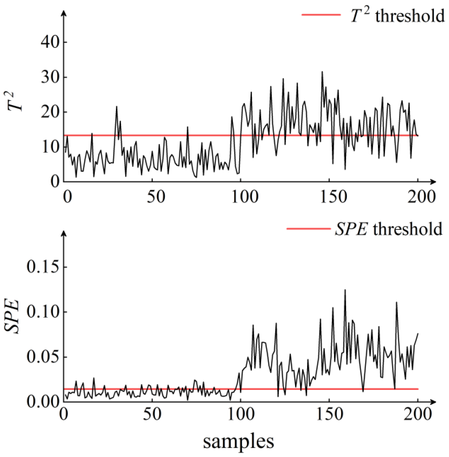
2.2. Online Monitoring and Diagnosis

After training, the monitoring model can be used for online monitoring. For the newly input variable sample ${\mathit{x}}_{new}\in {\mathit{R}}^{1\times m}$, the data standardization processing should be unified with the training model at first. When the PLS algorithm is used for monitoring, a projection direction matrix $\mathit{R}$ ($\mathit{R}=\left[{\mathit{r}}_1,{\mathit{r}}_2,\dots ,{\mathit{r}}_A\right]$) of data matrix $\mathit{X}$ should be introduced into the basis of the training model, $\mathit{T}=\mathit{X}\mathit{R}$. Therefore, we can directly find the matrix of the principal components.

Measurement sample scores and residuals:

$$\{\begin{array}{c}{\mathit{t}}_{\mathrm{new}}={\mathit{x}}_{\mathrm{new}}\mathit{R}\hfill \\ {\tilde{\mathit{x}}}_{\mathrm{new}}={\mathit{x}}_{\mathrm{new}}\left(1-\mathit{P}{\mathit{R}}^{\mathrm{T}}\right)\hfill \end{array}$$

(12)

Describing the fluctuation of the system and residual by $T^2$ and $SPE$ statistics.

$$\{\begin{array}{c}{T}^2={\mathit{t}}_{\mathrm{new}}^T{\mathit{\Lambda }}^{-1}{\mathit{t}}_{\mathrm{new}}\hfill \\ SPE={\tilde{\mathit{x}}}_{\mathrm{new}}{}^2\hfill \end{array}$$

(13)

where $\mathit{\Lambda }$ is the covariance matrix of the training model sample scores, $\mathit{\Lambda }=\frac{{\mathit{T}}^{\mathrm{T}}\mathit{T}}{n-1}$.

The control limits of the two statistics are calculated as follows.

$$\{\begin{array}{c}{T}_{\mathrm{ucl}}^2\left(\alpha \right)=\frac{A\left(n^2-1\right)}{n\left(n-A\right)}{F}_{A,n-A,\alpha }\\ SP{E}_{\mathrm{ucl}}^2\left(\alpha \right)=g{\chi }_{h,\alpha }^2\hfill \end{array}$$

(14)

where $g=\frac{S}{2\mu }, h=\frac{2{\mu }^2}{S}$, $\mu$ is the mean of the $SPE$ statistic, and $S$ is the variance.

KPLS algorithm is used for online monitoring. Firstly, the kernel matrix of samples is constructed as follows:

$${\mathit{K}}_{\mathrm{new}}=\left[k\left({\mathit{x}}_1,{\mathit{x}}_{\mathrm{new}}\right),k\left({\mathit{x}}_2,{\mathit{x}}_{\mathrm{new}}\right),\cdots ,k\left({\mathit{x}}_n,{\mathit{x}}_{\mathrm{new}}\right)\right]\in {\mathit{R}}^{1\times n}$$

(15)

The new kernel matrix is centralized as follows:

$${\overline{\mathit{K}}}_{\mathrm{new}}={\mathit{K}}_{\mathrm{new}}-{\mathit{I}}_N\overline{\mathit{K}}-{\mathit{K}}_{\mathrm{new}}{\mathit{I}}_n+{\mathit{I}}_N\overline{\mathit{K}}{\mathit{I}}_n$$

(16)

where ${\mathit{I}}_N=\frac{1}{n}\left[1\cdots 1\right]\in {\mathit{R}}^{1\times n}$.

The score matrix of the sample to be tested is calculated as follows:

$${\mathit{t}}_{\mathrm{new}}={\overline{\mathit{K}}}_{\mathrm{new}}\mathit{U}{\left({\mathit{T}}^T\overline{\mathit{K}}\mathit{U}\right)}^{-1}$$

(17)

The calculation of $T^2$ statistic, control limit of the KPLS online monitoring model and control limit of $SPE$ is the same as PLS. The $SPE$ statistic is calculated by a simple method as follows:

$$SPE={\displaystyle \sum }_{i=1}^n{\mathit{t}}_i^2-{\displaystyle \sum }_{i=1}^A{\mathit{t}}_i^2$$

(18)

In engineering application, when the two indexes are within the allowable range, the process runs normally. When both indexes exceed the standard, it is judged that the current process is uncontrollable. Only a certain statistical index exceeds the standard, and an early warning appears.

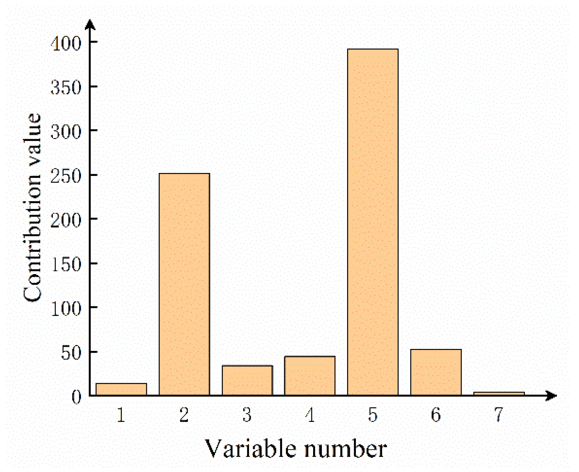
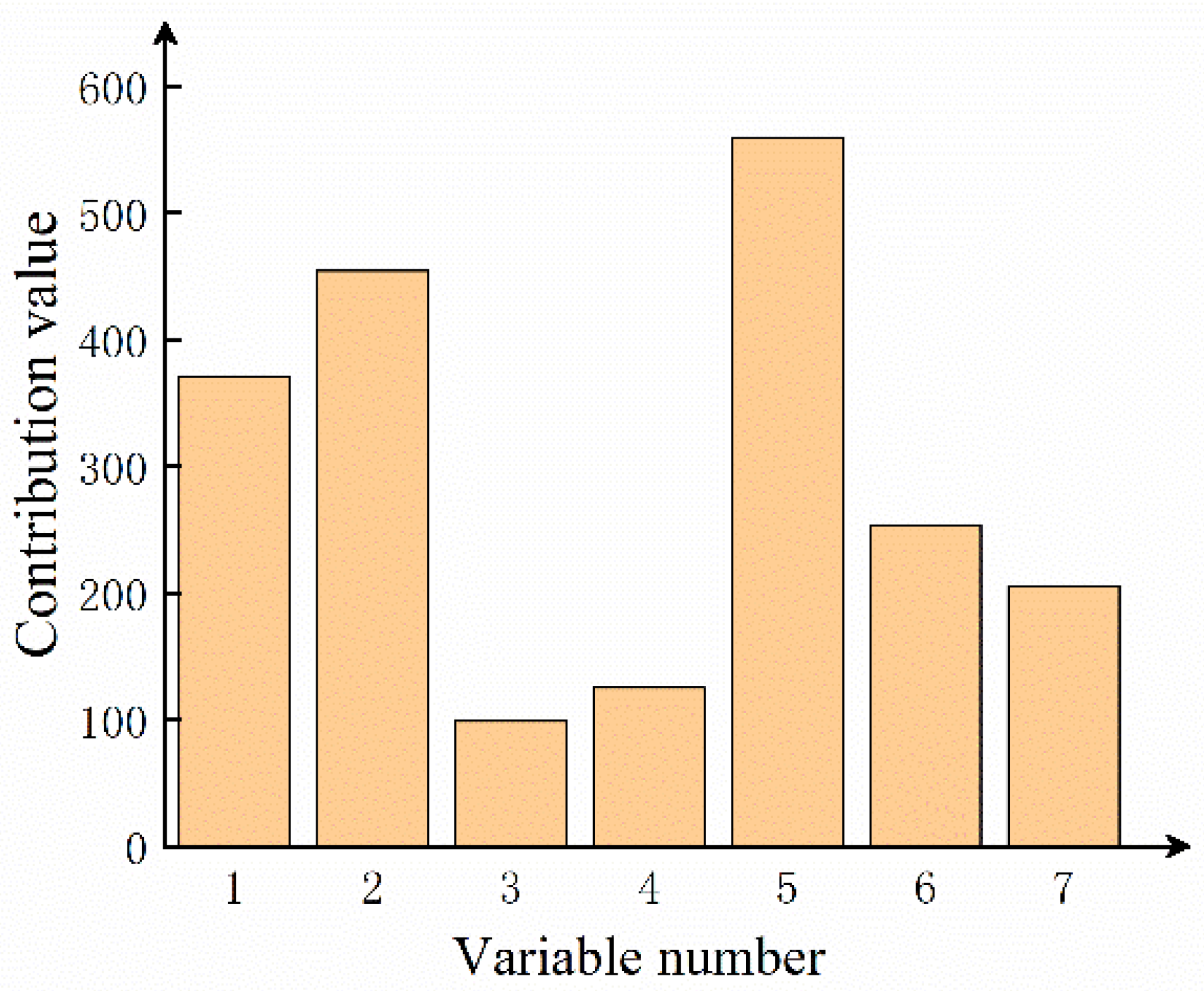
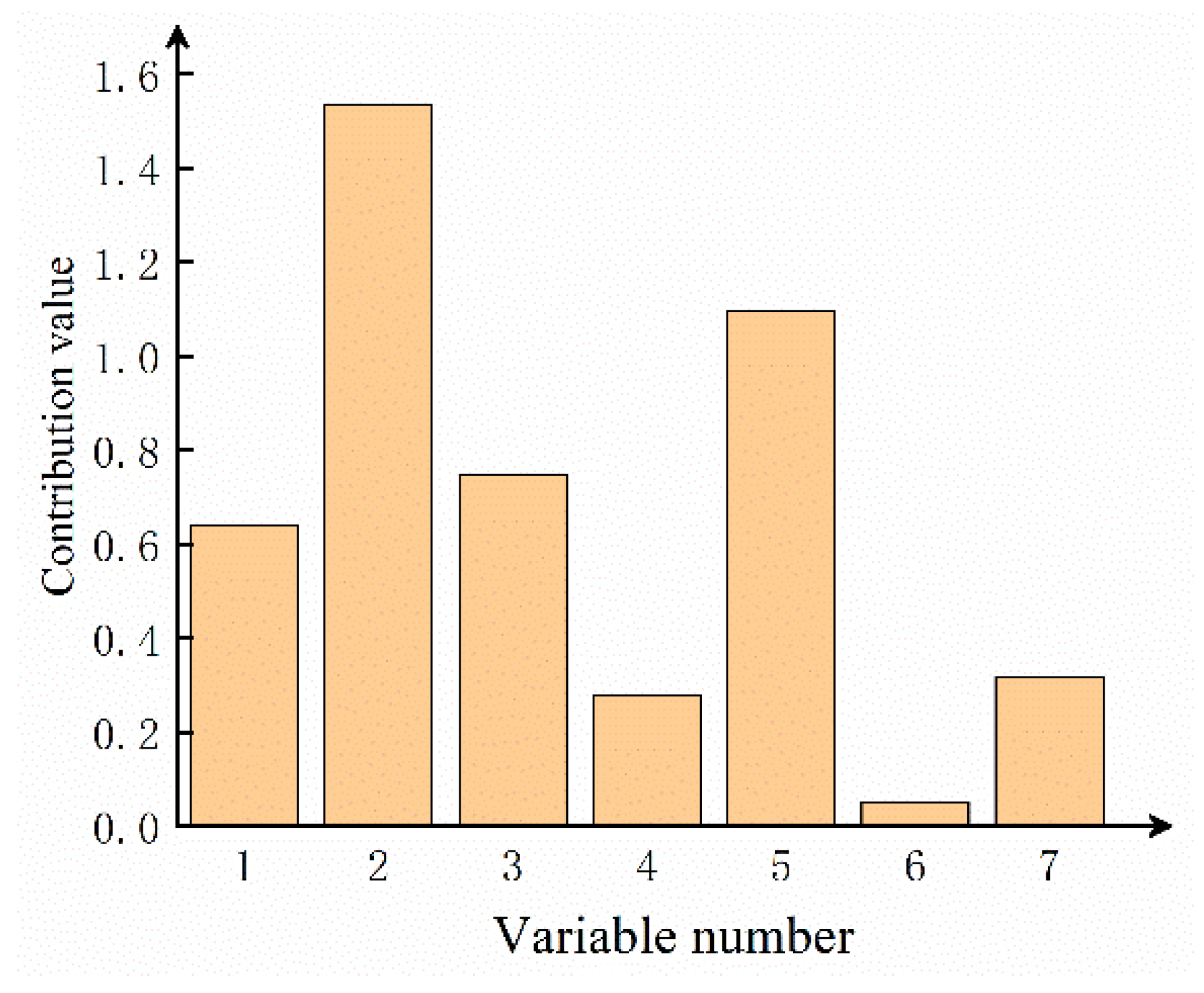
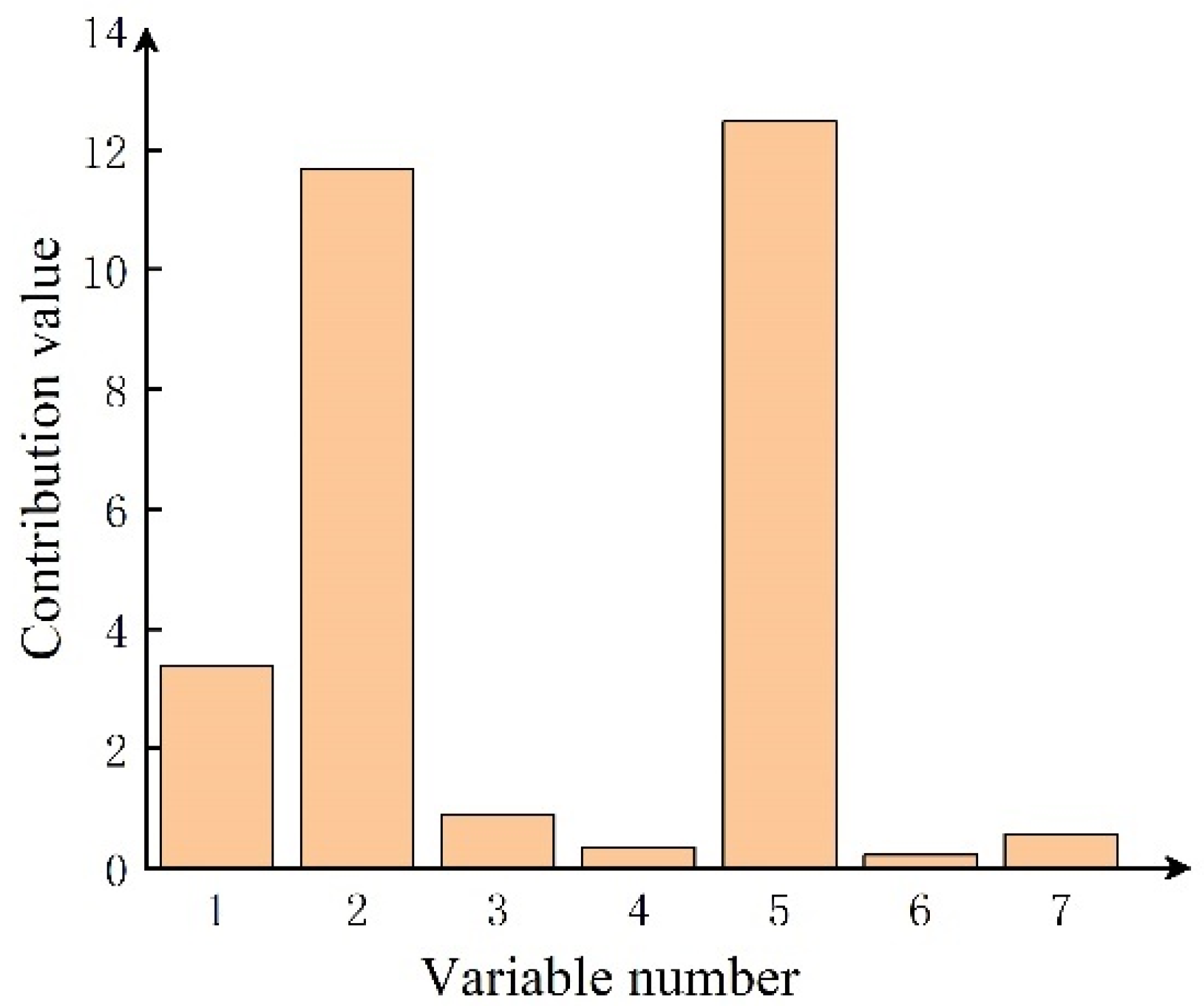
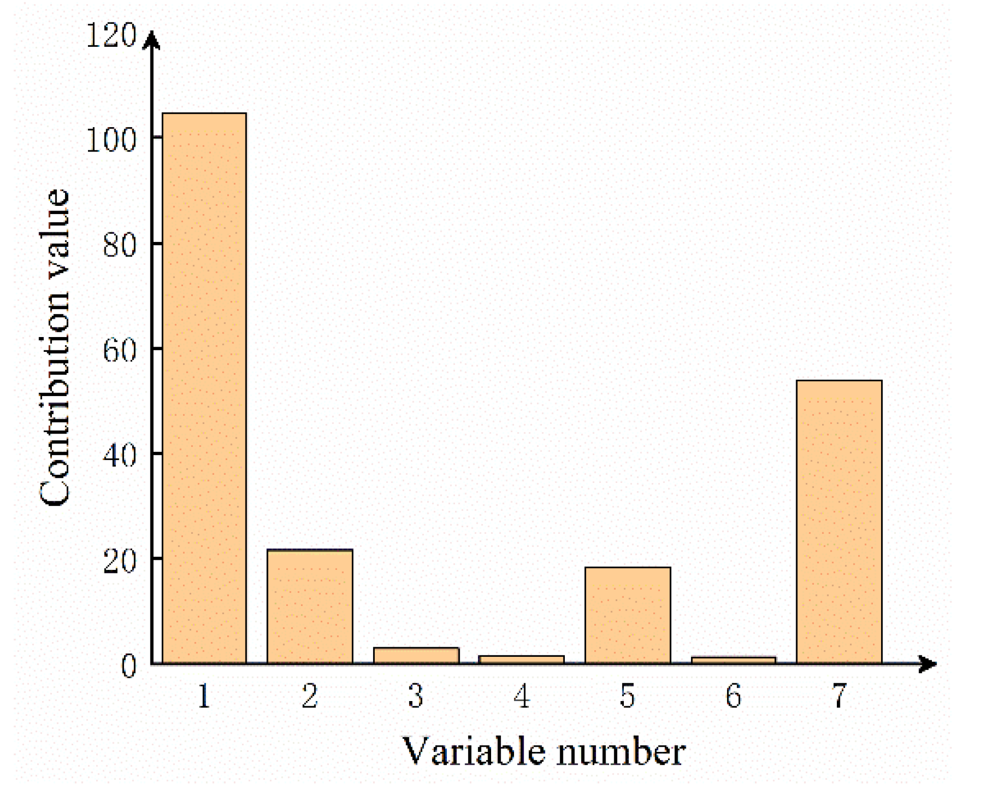
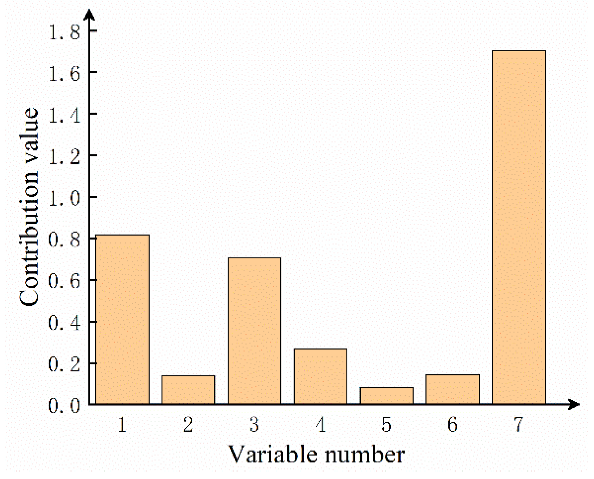
2.3. Fault Diagnosis Based on Nonlinear Contribution Plot

In this paper, the contribution plot method was used to diagnose and analyze the statistical data. The total contribution of the i-th sample to the j-th variable is calculated as follows:

$$cont{r}_{ij}^{SPE}={\left(x_{ij}-{\widehat{x}}_{ij}\right)}^2$$

(19)

where $x_{ij}$ is the monitored value of the $j$ variable at the $i$ sample point, and ${\widehat{x}}_{ij}$ is the predicted value of the $j$ variable at the $i$ sample point.

In order to make the relative contribution graph more effective in dealing with a complex production process, the expectation factor is added to the traditional contribution graph, as follows:

$$Rcont{r}_{ij}^{SPE}=\frac{cont{r}_{ij}^{SPE}}{E\left[cont{r}_{ij}^{SPE}\right]}$$

(20)

The nonlinear contribution plot calculates the contribution of each variable of each sample point to the monitoring index so as to find out the main fault variables and complete the diagnosis of abnormal sample points in the monitoring process. The new input sample ${\mathit{x}}_{\mathrm{new},\mathrm{r}}\in {\mathit{R}}^{1\times m}$ ($r=1,2,\dots ,m$. used to distinguish different process variables) and the Gaussian radial basis kernel function are used in this paper; then the partial derivative of the kernel matrix ${\mathit{K}}_{\mathrm{new}}$ of the new input point with respect to each variable is as follows:

$${\mathit{K}}_{\mathrm{new},i}^{\prime }=-\frac{1}{\sigma }{\left({\mathit{x}}_{\mathrm{new},\mathrm{r}}-{\mathit{x}}_{i,r}\right)}^{2}k\left({\mathit{x}}_{\mathrm{new}},{\mathit{x}}_i\right)$$

(21)

where $x_{i,r}$ is the $i$ element of the $r$ variable in the training sample, $i=1,2,\dots ,n$. $\sigma$ is constant.

The partial derivative of the centralized kernel matrix ${\mathit{K}}_{\mathrm{new}}$ with respect to each variable is as follows:

$${\overline{\mathit{K}}}_{\mathrm{new},i}^{\prime }={\mathit{K}}_{\mathrm{new},i}^{\prime }-{\mathit{K}}_{\mathrm{new},i}^{\prime }{\mathit{I}}_n$$

(22)

Using the latent variable matrix and kernel matrix calculated in the training model and monitoring model, the $SPE$ contribution value of each variable is calculated as follows:

$$con{t}_r^{SPE}=\mathbf{\left|}-\frac{2}{n}{\displaystyle \sum }_{i=1}^n{\overline{\mathit{K}}}_{\mathrm{new},i}^{\prime }-{\overline{\mathit{K}}}_{\mathrm{new}}^{\prime }\left(2\mathit{T}{\mathit{t}}_{\mathrm{new}}^{\mathrm{T}}-\mathit{U}{\mathit{T}}^{\mathrm{T}}\overline{\mathit{K}}\mathit{T}{\mathit{t}}_{\mathrm{new}}^{\mathrm{T}}\right)+{\mathit{t}}_{\mathrm{new}}{\mathit{T}}^{\mathrm{T}}\overline{\mathit{K}}\mathit{T}{\mathit{U}}^{\mathrm{T}}{\overline{\mathit{K}}}^{\prime }{}_{\mathrm{new}}^{\mathrm{T}}\mathbf{\right|}$$

(23)

where ${\overline{\mathit{K}}}_{\mathrm{new}}^{\prime }$ is the partial derivative kernel matrix composed of partial derivative vector ${\overline{\mathit{K}}}_{\mathrm{new},i}^{\prime }$.

3. Thickness Control and Static Comprehensive Analysis of Rolling Process

3.1. Mechanism Analysis of Aluminum Alloy Strip Rolling Process

Strip production is a complex industrial process with multi-process cooperation. In this process, melting, casting, rolling and other processes are concentrated in one production line as shown in Figure 2. The strip rolling stage is composed of multiple stand units, and the rolling at this stage requires the coordination of multiple stands. The process unit of each working procedure in the production process is complex. The strip quality is inherited among the working procedures. In this paper, the rolling process is taken as the research object, and the quality monitoring model is established to achieve the goal of strip thickness monitoring.

In the rolling stage, the metals undergo elastic-plastic deformation under the action of the force between the rolls. As a result of elastic deformation, the actual reduction of the roll is reduced, and the exit thickness of the rolled piece is greater than the value of the no-load roll gap as shown in Figure 3. Therefore, strip thickness and elastic flattening constitute the basis of strip thickness control.

In order to optimize the mechanism of the strip thickness quality monitoring data model, this part analyzes the strip thickness control mechanism. Based on the change principle of the elastic-plastic curve, the related control factors of strip thickness are analyzed. Under the actual rolling conditions, the roll gap is closely related to the thickness. In order to describe the relationship between the total elastic deformation of the rolling mill and rolling pressure, the spring equation of the rolling mill is established [34]. According to the elastic curve, the thickness of the rolled exit strip is shown in the following formula.

$$h=s_0+∆s=s_0+\frac{P}{K}$$

(24)

$$K=P/\left(h-s_0\right)$$

(25)

where $s_0$ is the empty roll gap, $∆s$ is the deformation of stand under rolling force, $P$ is the rolling pressure, and $K$ is the stiffness coefficient of the rolling mill.

For the longitudinal thickness of the strip, the longitudinal stiffness of the rolling mill is mainly considered. In addition to the influence of the state of the incoming rolled piece, the longitudinal thickness of the strip will change as long as the rolling pressure fluctuation is involved in the rolling process. In order to eliminate the thickness deviation caused by disturbance factors, the intersection point of two characteristic curves is returned to the preset point. This section briefly introduces the corresponding plate thickness control means [35].

When the thickness of incoming material fluctuates greatly, the original rolling conditions cannot meet the requirement of rolling out thickness. At this time, changing the size of the reduction offsets the rolling factor or the thickness deviation caused by rolling pressure fluctuation due to the interference of the rolling mill system.

As shown in Figure 4 the expected rolling thickness is $h_0$. Other conditions of the rolled piece remain unchanged; thus the slope of the plastic curve $B$ remains the same. However, the increase in blank thickness makes the curve shift to $B^{\prime }$ to the right, intersects with the original rolling mill elastic curve $A$ to $h_1$, which leads to the corresponding thickness deviation of $\left(h_1-h_0\right)$. At this time, the thickness control system of the rolling mill reacts by increasing the reduction and reducing the roll gap, and thus the elastic curve of the rolling mill shifts to the position $A^{\prime }$. The abscissa of the intersection point comes to $h_0$ again so as to eliminate the thickness deviation.

On the other hand, when the thickness of the incoming material is normal, there are some problems such as uneven temperature and fluctuation of hardness or microstructure. When the deformation resistance of the rolled piece is affected, the slope of the plastic curve of the rolled piece will change as shown in Figure 5. At this time, the deformation resistance of the rolled piece increases, and thus the slope of the original plastic curve increases from $B$ to $B^{\prime }$, and the rolling thickness obtained by intersecting with the original elastic curve $A$ of the rolling mill increases from $h_0$ to $h_1$. At this time, the rolling mill increases the reduction and adjusts the elastic curve $A$ to the position of $A^{\prime }$, and thus the rolling thickness returns to the expected value.

By adjusting the tension to change the slope of the plastic curve of the rolled piece, the intersection of the plastic curve and the elastic curve of the rolling mill can be adjusted to offset the influence of other factors on the rolling thickness. The front and back tension of the rolling mill reduce the positive pressure on the roll, resulting in the reduction in rolling force. The relationship between tension and rolling force is as follows.

$$P_q=P[1-\frac{1}{K}\left(m_1{q}_1+m_2{q}_2\right)]$$

(26)

where $m_1$ and $m_2$ are the influence factor of tension at the entrance and exit of the rolling mill, and $q_1$ and $q_2$ are the strip tension at the inlet and outlet of the mill, respectively. $P_q$ is the rolling pressure with tension, $P$ is the rolling pressure without tension, and $K$ is the deformation resistance.

As shown in Figure 6, with the increase in tension, the plastic curve of the rolled piece can be adjusted from B to $B^{\prime }$ (slope increases). Thus, the abscissa of the intersection point with the elastic curve $A$ is adjusted from $h_1$ to $h_2$. The purpose of plate thickness adjustment can be achieved without changing the size of the roll gap. From the practical application, the tension adjustment method has the characteristics of fast response and good effect. It is widely used in cold-rolled strips. The adjustment of rolling speed also affects the thickness of the plate at the outlet. The main influence is that the change in speed causes the fluctuation of the variables such as tension, friction coefficient, rolling temperature and bearing oil film thickness so that the rolling pressure can also be changed.

Through the analysis of the above thickness control principle, it is known that the strip rolling system is a complex system with multivariable coupling, and there is a close relationship between process variables and equipment variables [36]. In order to optimize the mechanism of the data model, the plate thickness of the stable rolling process was analyzed based on the static comprehensive analysis theory.

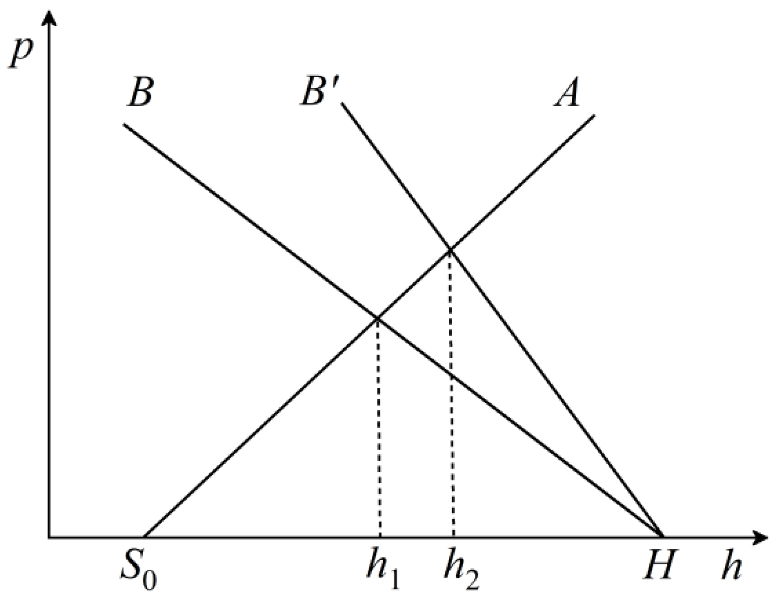
3.2. Static Synthesis Analysis of Steady-State Rolling

Taking the longitudinal plate thickness as an example, the differential of rolling mill bounce is as follows:

$$\delta h=\delta S+\frac{\delta P}{K_m}+\frac{\delta F}{K_F}$$

(27)

where $K_m$ is the total stiffness of the rolling mill, $K_F$ is the longitudinal stiffness of the roll system corresponding to the bending force of the roll, $P$ is measured rolling force, $S$ is the initial roll gap value, and $F$ is roll bending force.

The rolling force is regarded as a function of incoming thickness $H$, rolled thickness $h$, deformation resistance $K$, and front and rear tensile stress $q_f$, $q_b$, ignoring the rolling speed fluctuation and strip width variation, as follows:

$$\delta P=f\left(H,h,K,q_f,q_b\right)$$

(28)

The incremental form of rolling force is as follows:

$$\delta P=\frac{\partial P}{\partial H}\delta H+\frac{\partial P}{\partial h}\delta h+\frac{\partial P}{\partial K}\delta K+\frac{\partial P}{\partial q_f}\delta q_f+\frac{\partial P}{\partial q_b}\delta q_b$$

(29)

The mathematical model of incremental thickness is as follows:

$$\delta h=\left(C_H\delta H+C_K\delta K\right)+\left(C_S\delta S+C_F\delta F\right)+\left(C_{q_f}\delta q_f+C_{q_b}\delta q_b\right)$$

(30)

The influence coefficients of each variable are shown in

Table 1. Influence coefficients of some variables.

Index	${\mathit{C}}_{\mathit{H}}$	${\mathit{C}}_{\mathit{K}}$	${\mathit{C}}_{\mathit{S}}$	${\mathit{C}}_{\mathit{F}}$	${\mathit{C}}_{\mathit{q}}$	${\mathit{C}}_{\mathit{q}}$
Expression	$\frac{1}{K_m+Q}\frac{\partial P}{\partial h_0}$	$\frac{1}{K_m+Q}\frac{\partial P}{\partial K}$	$\frac{K_m}{K_m+Q}$	$\frac{K_m}{\left(K_m+Q\right)K_F}$	$\frac{1}{K_m+Q}\frac{\partial P}{\partial q_f}$	$\frac{1}{K_m+Q}\frac{\partial P}{\partial q_b}$

Note: $Q=-\frac{\partial P}{\partial h}$ is the plastic stiffness coefficient of rolled piece and is called the slope value of rolled piece plastic curve.

.

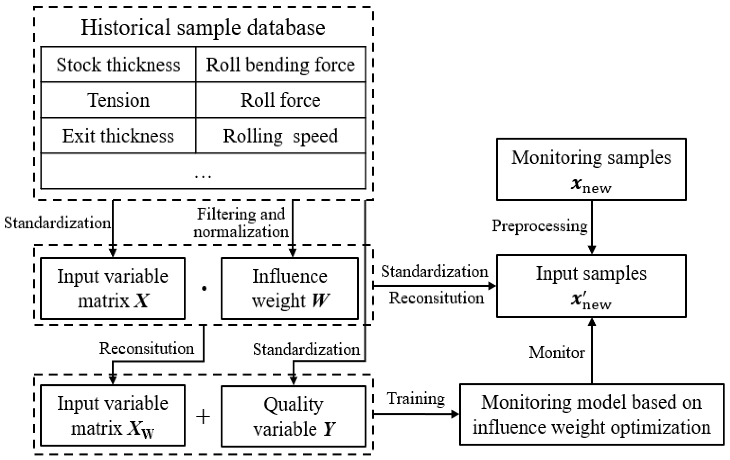
4. Monitoring Method Based on Influence Weight Optimization

4.1. Influence Coefficient Calculation of Data Set

In this paper, the influence coefficient obtained from the static characteristic analysis is used to interpret the input variables of the data model from the perspective of the rolling process mechanism model so that the monitoring model can achieve higher fault detection accuracy.

Let the sample data matrix of the rolling process be $\mathit{X}=\left({\mathit{X}}_1,{\mathit{X}}_2,\dots ,{\mathit{X}}_{m^{\prime }}\right)\in {\mathit{R}}^{n\times m^{\prime }}$. The number of process variables is $m^{\prime }$, and $n$ is the sample size. In this section, on the basis of a large number of historical samples, the partial differential coefficient is calculated by means of chord tangent within a small variation range of variables.

Divide the historical data matrix $\mathit{X}$ into $N$ equal parts according to capacity: ${\mathit{X}}^{\left(1\right)},{\mathit{X}}^{\left(2\right)},\mathbf{\dots },{\mathit{X}}^{\left(N\right)}$. Calculate the mean value of each variable in each equal part as follows:

$${\overline{\mathit{X}}}^{\left(i\right)}=\left({\overline{X}}_1^{\left(i\right)},{\overline{X}}_2^{\left(i\right)},\dots ,{\overline{X}}_{m^{\prime }}^{\left(i\right)}\right)$$

(31)

where ${\overline{\mathit{X}}}_{m^{\prime }}^{\left(i\right)}$ is the mean of the $m^{\prime }$ variable in the $i$ equal fraction, $i=1,2,\dots ,N$.

The mean vector ${\overline{\mathit{X}}}^{\left(i\right)}$ was obtained. In order to illustrate the use of $\partial P$ to refer to the change value of rolling force, the partial differential values of the corresponding variables of each adjacent two vectors were taken as follows:

$$\frac{\partial {\overline{X}}_j^{\left(k\right)}}{\partial P^{\left(k\right)}}=\frac{{\overline{X}}_j^{\left(k+1\right)}-{\overline{X}}_j^{\left(k\right)}}{\partial P^{\left(k\right)}}$$

(32)

where $k=1,2,\dots ,N-1$; $j=1,2,\dots ,m^{\prime }$.

The mean value of $\left(N-1\right)$ partial differential values of each relevant variable is calculated, and the partial differential coefficients are obtained as follows:

$$\frac{\partial {\mathit{X}}_j}{\partial \mathit{P}}=\frac{1}{k}{\displaystyle \sum }_1^k\frac{\partial {\overline{X}}_j^{\left(k\right)}}{\partial P^{\left(k\right)}}$$

(33)

Combined with the influence coefficient expression of the quality fluctuation of each variable strip in Section 3.2 static comprehensive analysis of steady rolling, the final influence coefficient is obtained as follows:

$$\mathit{C}=\left(C_1,C_2,\dots ,C_m\right)\in {\mathit{R}}^{1\times m}$$

(34)

where $m$ is the number of process variables.

4.2. KPLS Monitoring Method Based on Influence Weight W Optimization

Based on a data-driven algorithm, data feature is the direct information source of the monitoring model. Traditional data preprocessing cannot adapt to specific working conditions and cannot highlight the influence of different variables. According to the calculation of influence coefficients in Section 4.1, the influence coefficients of some variables obtained based on the historical data set of a certain rolling process are shown in

Table 2. An example of the influence coefficient of a course calculation.

Index	Exit Velocity	Back Tension	Front Tension	Entry Thickness
Partial differential	53,141.42	4.42	1.57	18,534.48
Influence coefficient	0.044	3.70 × 10−6	1.31 × 10−6	0.02
Mean value	5.78	18,829.54	15,846.74	0.28
Influence weight	0.254	0.070	0.021	0.004

. It can be found that due to the different orders of magnitude of different variables, their influence coefficient values often differ greatly. In the algorithm model, the difference in the order of magnitude of data becomes smaller after standardization, and thus the obtained influence coefficient cannot be directly used to distinguish the influence of variables. In this paper, the value of the influence coefficient is multiplied by the mean value $\overline{\mathit{X}}$ of the corresponding variable, which is used as the optimization weight W of the follow-up monitoring model.

$$\mathit{W}=\mathit{C}{\overline{\mathit{X}}}^{\mathrm{T}}$$

(35)

The overall optimization strategy is shown in Figure 7, and the training process of the monitoring model is shown on the left side of the figure. Firstly, input variable matrix $\mathit{X}$ and quality variable matrix $\mathit{Y}$ are selected from the historical sample database and standardized for use, respectively. A small section of variable samples and the corresponding rolling force were selected from the database to construct the influence weight $\mathit{W}$. Then, the normalized input matrix is reconstructed as ${\mathit{X}}_W$ through matrix dot product calculation. Finally, the monitoring model is trained by using the above input and output matrices according to the corresponding KPLS algorithm steps.

In the figure above, the online monitoring process of the optimization model is shown on the right. The input sample ${\mathit{x}}_{\mathrm{new}}$ of real-time monitoring should correspond to the input sample of the training model after preprocessing. Firstly, the new input samples are standardized according to the data characteristics of the input matrix in the training process. Then the influence weight matrix is used to reconstruct the new input samples to obtain ${\mathit{x}}_{\mathrm{new}}^{\prime }$. Finally, the sample is kernel-mapped and centralized according to the online monitoring steps of the KPLS model. The trained monitoring model is used to complete the verification monitoring.

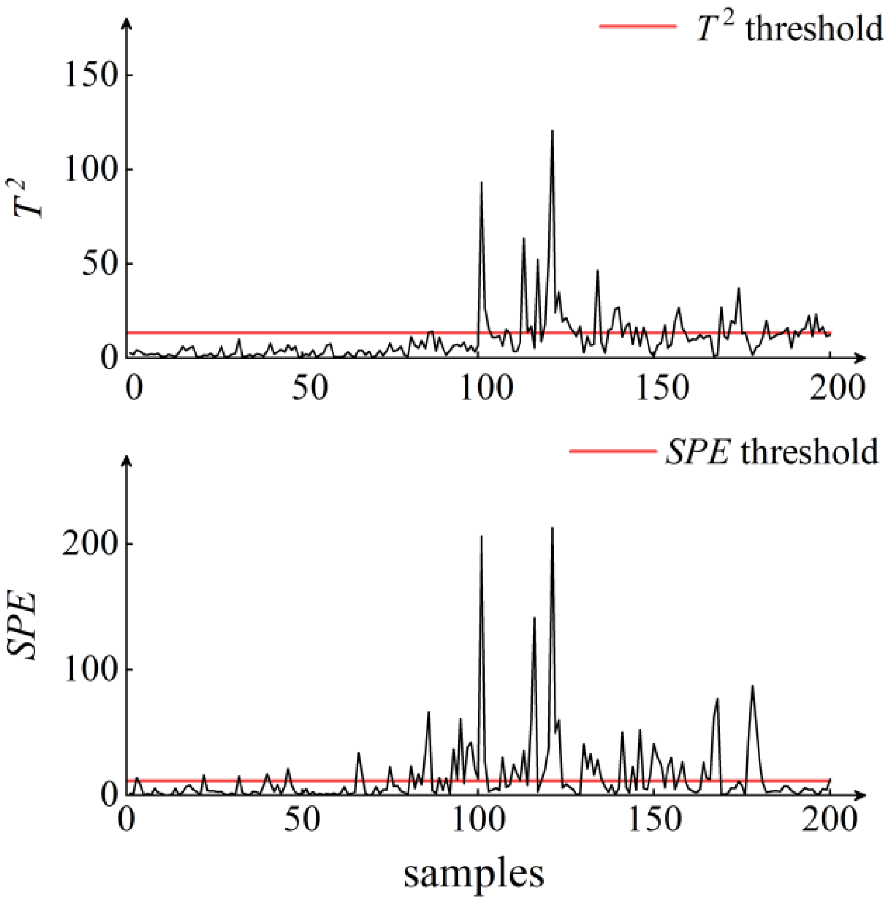
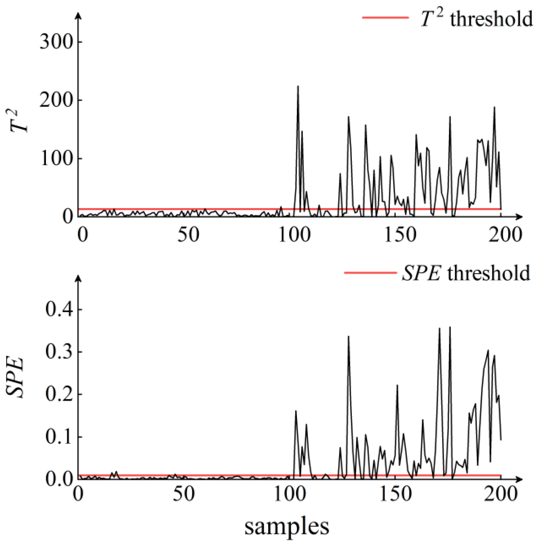
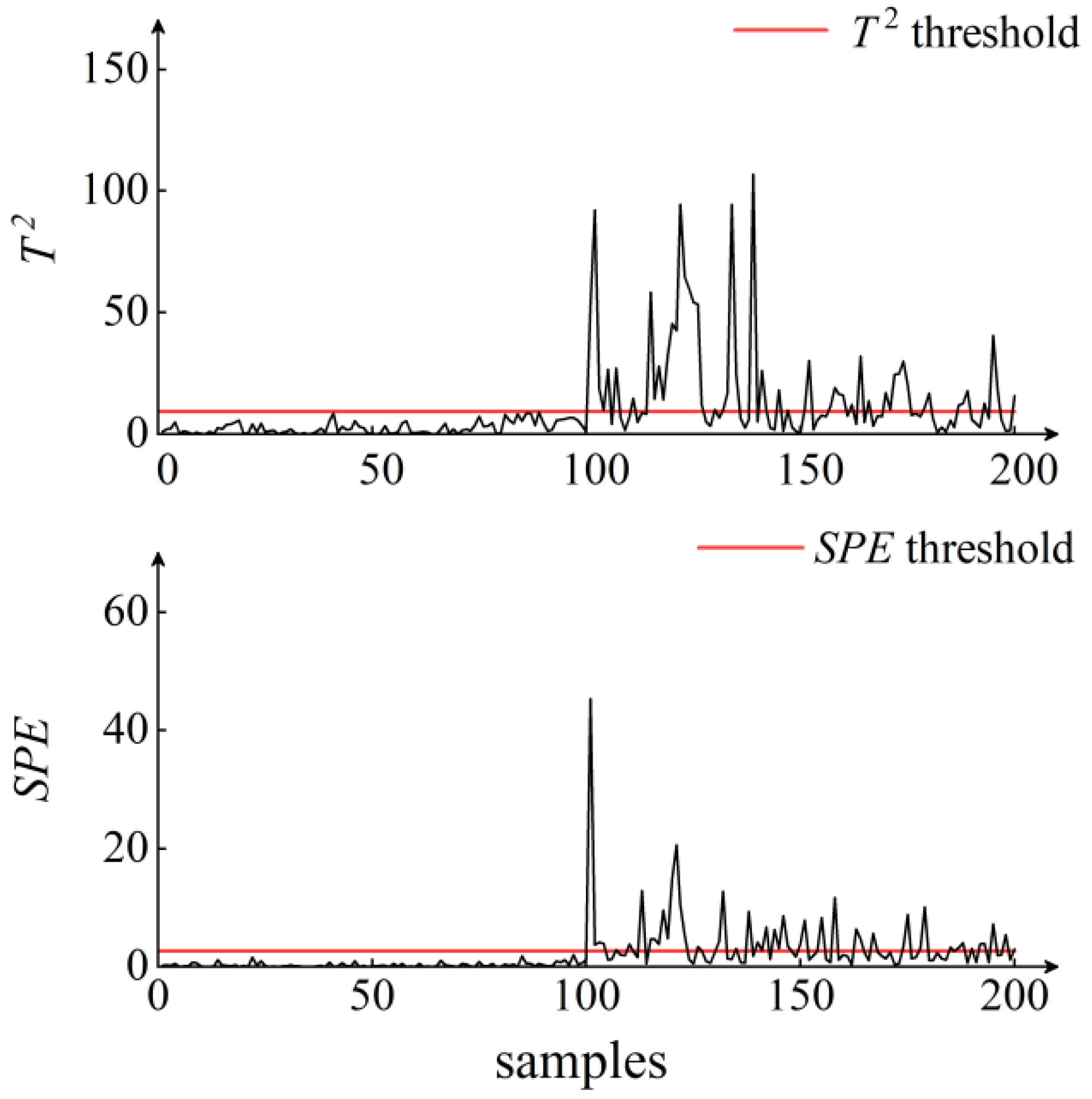
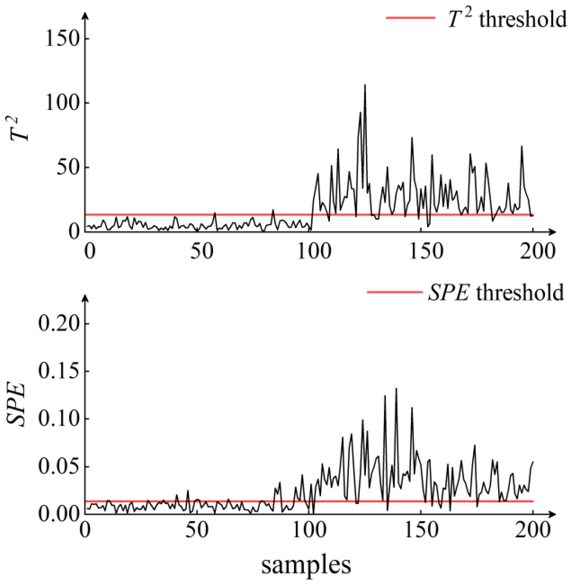
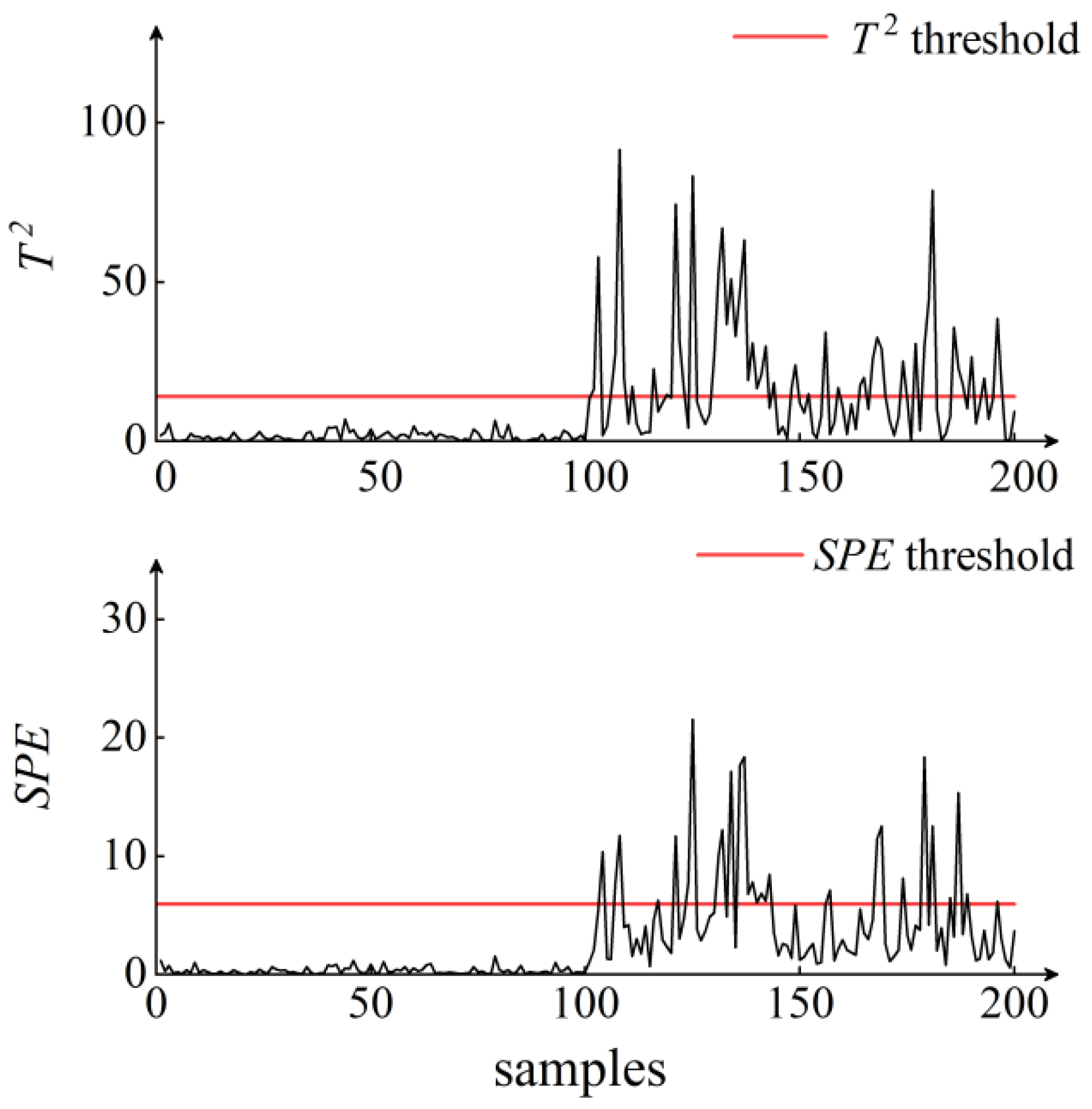
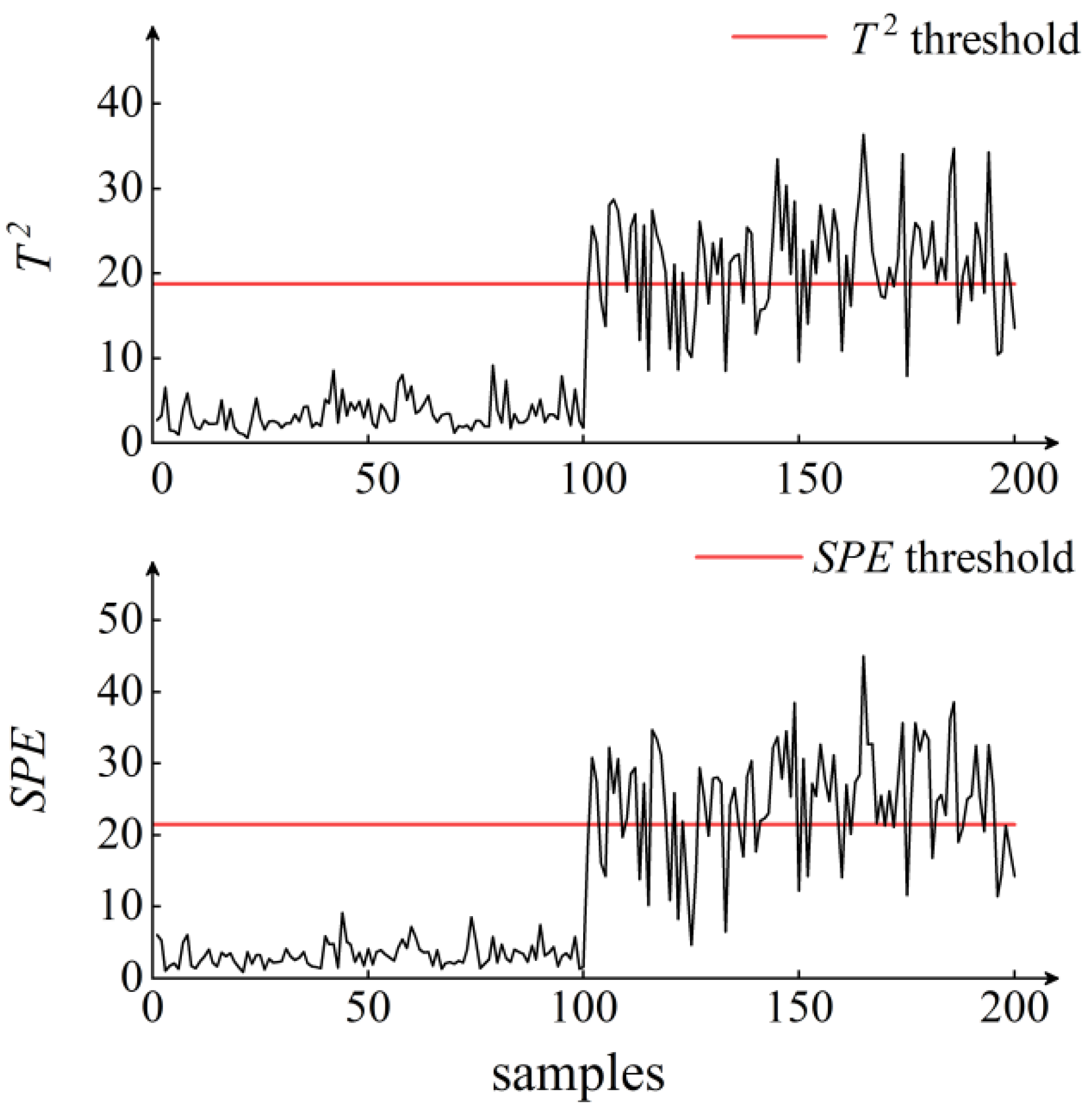
5. Results and Discussion

In order to illustrate our point of view further, we use the simulation data that come from the rolling production data of a 2800 mm cold rolling mill. The process variables included: roll gap value, roll bending force, entry speed, exit speed, incoming material thickness, front tension and back tension. Mass variable is the pass exit thickness of the strip.

A total of 1200 sets of production data samples were collected, among which 800 sets of normal operation data were used for training the offline model. The other 400 sets of data were used for the online monitoring model. Monitoring sample 1 included 100 sets of normal samples and 100 sets of fault samples, among which the default fault source was the transmission system fluctuation of the rolling mill. Monitoring sample 2 contains 100 groups of normal samples and 100 groups of fault samples, among which the default fault source is the uneven thickness of incoming materials.

The cumulative variance contribution rate is calculated using the sample data, as shown in

Table 3. Calculation of cumulative variance contribution rate.

Component Number	1	2	3	4	5	6	7
Variance contribution rate %	39.02	61.87	80.67	89.93	95.69	99.38	100

. In order to pursue calculation efficiency and take into account the accuracy of the model, the variance contribution of nearly 90% can be obtained when the number of principal components is set as 4.

The monitoring model is trained according to the modeling process of the PLS algorithm. The projection direction matrix $\mathit{R}$ of training is used to project each group of monitoring samples to obtain a new principal component and residual component. Statistical index $T^2$ and SPE are constructed, respectively. The online monitoring simulation diagram of the monitoring model based on the PLS algorithm is finally obtained. Radial basis function is used to carry out simulation monitoring based on the KPLS algorithm, and cross-validation was used to determine the kernel parameter $\sigma =3.5$.

The influence weight coefficient of strip thickness monitoring simulation based on optimization model as shown in

Table 4. Simulation calculation of influence weight.

Index	Entry Velocity	Exit Velocity	Front Tension	Back Tension	Roll Gap	Roll Bending Force	Entry Thickness
Partial differential	4494.08	7166.41	11.13	19.52	-	-	123,513.80
Influence coefficient	0.08	0.01	2.04 × 10−5	3.52 × 10−5	0.014	4.80 × 10−6	0.22
Mean value	10.58	13.57	15,828.13	18,820.76	0.72	146.36	0.28
Influence weight	0.85	0.14	0.32	0.66	0.01	0.007	0.06

. W-KPLS is used for online monitoring of sample 1 and compared with other methods. The simulation results of online monitoring are shown in the figure. As shown in Figure 8, using the traditional PLS method for monitoring, the monitoring index of sample 1 exhibits an obvious overrun phenomenon in the fault sample number 101–140 with a high detection rate. However, there is a lack of fault point monitoring around 140–200. For the monitoring results of KPLS in Figure 9, the fault detection rate of this method is significantly higher than that of PLS, but there are still a few missing points. In order to improve the fault detection rate, the monitoring method based on influence weight optimization is used for monitoring, and the results are shown in Figure 10 and Figure 11. We can see that the optimized monitoring method is better than the traditional monitoring method.

Online monitoring simulation for monitoring sample 2 is shown in Figure 12, Figure 13, Figure 14 and Figure 15. From the monitoring results of the following four methods for sample 2, the recognition rate of the W-KPLS monitoring model in fault sample points is greatly improved compared with the traditional algorithm. As shown in Figure 15, W-KPLS monitoring is used to reduce the missing rate of sample points. The feasibility of W-KPLS is verified by monitoring two samples with four methods. By fusing the mechanism model, the accuracy of traditional monitoring methods is improved.

The detailed fault detection rate statistics of the monitoring model based on the four algorithms for the two groups of monitoring samples are shown in

Table 5. Statistics of fault detection rate.

Monitoring Algorithms		PLS	W-PLS	KPLS	W-KPLS
Sample 1	Early warning rate %	69	72	75	99
	Alarm rate %	22	37	58	75
Sample 2	Early warning rate %	57	74	82	96
	Alarm rate %	20	62	40	68

. When the monitored sample exceeds one of the T² or SPE control lines, an early warning will be generated. An alarm indication will be issued if it exceeds two control limits at the same time. According to the control limit, the overall fault detection rate of the W-PLS algorithm is improved compared with that of the PLS algorithm, but it cannot meet the monitoring requirements. The data points of the W-KPLS algorithm whose $T^2$ and $SPE$ monitoring indexes simultaneously exceed the limit account for 75% and 68%, respectively, which are the highest among the four algorithms. At the same time, compared with the KPLS algorithm before optimization, the detection rate of the W-KPLS algorithm is increased by about 20 percentage points. The proportion of data points reaching the early warning limit is also increased to over 95%.

The over-limit monitoring index is analyzed using the traditional contribution plot and relative contribution plot based on a linear algorithm and the contribution plot based on a nonlinear algorithm. Results for the first group of monitoring samples are shown in Figure 16, Figure 17 and Figure 18, and results for the second group of monitoring samples are shown in Figure 19, Figure 20 and Figure 21.

The fault of monitoring sample 1 is caused by rolling mill drive system fluctuation. Both linear contribution plots show that variable 5 (roll gap value) has the largest contribution value, followed by variable 2 (exit speed). However, the contribution plot diagnosis results of the nonlinear algorithm show that variable 2 (exit velocity) is the main fault variable, and variable 5 (roll gap value) is the secondary fault variable.

The quality fluctuation of sample 2 was caused by the uneven thickness of incoming material. The traditional contribution plot shows that the most contributing fault variables are variable 2 (outlet speed) and variable 5 (roll gap value). While the relative contribution plot shows that variable 1 (inlet speed) is the main fault variable, and the influence of variable 7 (incoming material thickness) is the second. The contribution plot based on the nonlinear algorithm shows that variable 7 (entry thickness) is the main influencing variable. Data related to the quality fluctuation of actual production status were collected and verified by the diagnostic method in this paper. By analyzing the contribution plot above, it can be seen that the diagnosis result based on a nonlinear contribution diagram is consistent with the on-site fault diagnosis result.

6. Conclusions

In this study, a kernel partial least squares monitoring method based on influence weight (W-KPLS) for quality-related monitoring was proposed for a nonlinear and dynamic process, which can help industrial sites to achieve more accurate monitoring and diagnosis of quality variables. This method adopts mechanism analysis and data fusion, which makes up for the problem that the traditional data monitoring model cannot explain the industrial process variables. Firstly, the traditional monitoring method for the complex process industry was introduced. After that, a nonlinear contribution plot was applied to the quality-related fault diagnosis process. Then, the mechanism model of strip thickness control was introduced. The influence of rolling process variables was studied by static comprehensive analysis. Finally, according to the influence coefficient, the weight matrix was constructed. The W-KPLS model was proposed for quality-related monitoring and diagnosis. We can see that the method works well for quality-related monitoring and diagnosis in the aluminum alloy cold strip mill process of Nanshan aluminum. The fault detection rate is improved by 20% compared with the traditional method. The proportion of data points reaching the early warning limit is increased to more than 95%.

References

1. Shao, J.; He, A.; Dong, G.; Chen, B.; Chen, J. Whole process quality management and control system of iron and steel based on industrial interconnection. Metall. Ind. Autom. 2020, 44, 8–16. (In Chinese) [Google Scholar]
2. Ma, L.; Dong, J.; Peng, K. A practical propagation path identification scheme for quality-related faults based on nonlinear dynamic latent variable model and partitioned Bayesian network. J. Frankl. Inst. 2018, 355, 7570–7594. [Google Scholar] [CrossRef]
3. Si, Y.; Wang, Y.; Zhou, D. Key-Performance-Indicator-Related Process Monitoring Based on Improved Kernel Partial Least Squares. IEEE Trans. Ind. Electron. 2021, 68, 2626–2636. [Google Scholar] [CrossRef]
4. Lan, T.; Tong, C.; Shi, X.; Luo, L. Dynamic statistical process monitoring based on generalized canonical variate analysis. J. Taiwan Inst. Chem. Eng. 2020, 112, 78–86. [Google Scholar] [CrossRef]
5. Said, M.; Taouali, O. Improved Dynamic Optimized Kernel Partial Least Squares for Nonlinear Process Fault Detection. Math. Probl. Eng. 2021, 2021, 6677944. [Google Scholar] [CrossRef]
6. Wang, G.; Li, J.D.; Sun, C.Y.; Jiao, J.F. Least Squares and Contribution Plot Based Approach for Quality-Related Process Monitoring. IEEE Access 2018, 6, 54158–54166. [Google Scholar] [CrossRef]
7. Ge, Z. Review on data-driven modeling and monitoring for plant-wide industrial processes. Chemom. Intell. Lab. Syst. 2017, 171, 16–25. [Google Scholar] [CrossRef]
8. Yan, P. Review on development of digital and intelligent metallurgical rolling equipment technology. J. Yanshan Univ. 2020, 44, 218–237. (In Chinese) [Google Scholar]
9. Hu, Z.; Wei, Z.; Sun, H.; Yang, J.; Wei, L. Optimization of Metal Rolling Control Using Soft Computing Approaches: A Review. Arch. Comput. Methods Eng. 2021, 28, 405–421. [Google Scholar] [CrossRef]
10. Kong, X.; Li, Q.; An, Q.; Xie, J. Quality-related fault detection based on the score reconstruction associated with partial least squares. Control. Theory Appl. 2020, 37, 2321–2332. (In Chinese) [Google Scholar]
11. Jing, F.; Feng, Y.; Zhang, Y.; Li, W. Diagnostic study on based thickness deviation of hot rolled strip based on optimized RT-PLS. J. Iron Steel Res. 2021, 33, 593–599. [Google Scholar] [CrossRef]
12. Zhang, K.; Hao, H.; Chen, Z.; Ding, S.X.; Peng, K. A comparison and evaluation of key performance indicator-based multivariate statistics process monitoring approaches. J. Process Control 2015, 33, 112–126. [Google Scholar] [CrossRef]
13. Jiao, J.; Zhen, W.; Wang, G.; Wang, Y. KPLS–KSER based approach for quality-related monitoring of nonlinear process. ISA Trans. 2020, 108, 144–153. [Google Scholar] [CrossRef] [PubMed]
14. Zhou, P.; Zhang, R.; Liang, M.; Fu, J.; Wang, H.; Chai, T. Fault identification for quality monitoring of molten iron in blast furnace ironmaking based on KPLS with improved contribution rate. Control Eng. Pract. 2020, 97, 104354. [Google Scholar] [CrossRef]
15. Jiang, Q.; Yan, X. Quality-Driven Kernel Projection to Latent Structure Model for Nonlinear Process Monitoring. IEEE Access 2019, 7, 74450–74458. [Google Scholar] [CrossRef]
16. Zhou, D.; Li, G.; Qin, S.J. Total projection to latent structures for process monitoring. AIChE J. 2009, 56, 168–178. [Google Scholar] [CrossRef]
17. Qin, S.J.; Zheng, Y. Quality-relevant and process-relevant fault monitoring with concurrent projection to latent structures. AIChE J. 2013, 59, 496–504. [Google Scholar] [CrossRef]
18. Peng, K.; Zhang, K.; You, B.; Dong, J. Quality-relevant fault monitoring based on efficient projection to latent structures with application to hot strip mill process. IET Control Theory Appl. 2015, 9, 1135–1145. [Google Scholar] [CrossRef]
19. Kong, X.; Cao, Z.; An, Q.; Xu, Z.; Luo, J. Review of partial least squares linear models and their nonlinear dynamic expansion models. Control Decis. 2018, 33, 1537–1548. [Google Scholar] [CrossRef]
20. Tang, Q.; Chai, Y.; Qu, J.; Fang, X. Industrial process monitoring based on Fisher discriminant global-local preserving projection. J. Process Control 2019, 81, 76–86. [Google Scholar] [CrossRef]
21. Zhang, C.; Peng, K.; Dong, J. A P-t-SNE and MMEMPM based quality-related process monitoring method for a variety of hot rolling processes. Control Eng. Pract. 2019, 89, 1–11. [Google Scholar] [CrossRef]
22. Jiang, Q.; Yan, X. Hierarchical monitoring for Multi-unit chemical processes based on Local-global correlation features. Acta Autom. Sin. 2020, 46, 1770–1782. [Google Scholar] [CrossRef]
23. Odiowei, P.; Yi, C. Nonlinear Dynamic Process Monitoring Using Canonical Variate Analysis and Kernel Density Estimations. IEEE Trans. Ind. Inform. 2010, 6, 36–45. [Google Scholar] [CrossRef] [Green Version]
24. Pilario, K.; Cao, Y.; Shafiee, M. Mixed kernel canonical variate dissimilarity analysis for incipient fault monitoring in nonlinear dynamic processes. Comput. Chem. Eng. 2019, 123, 143–154. [Google Scholar] [CrossRef] [Green Version]
25. Yu, H.; Khan, F. Improved latent variable models for nonlinear and dynamic process monitoring. Chem. Eng. Sci. 2017, 168, 325–338. [Google Scholar] [CrossRef]
26. Zhang, C.; Peng, K.; Dong, J. A nonlinear full condition process monitoring method for hot rolling process with dynamic characteristic. ISA Trans. 2021, 112, 363–372. [Google Scholar] [CrossRef]
27. Jiao, J.; Zhen, W.; Zhu, W.; Wang, G. Quality-Related Root Cause Diagnosis Based on Orthogonal Kernel Principal Component Regression and Transfer Entropy. IEEE Trans. Ind. Inform. 2021, 17, 6347–6356. [Google Scholar] [CrossRef]
28. Tian, W.; Ren, Y.; Dong, Y.; Wang, S.; Bu, L. Fault monitoring based on mutual information feature engineering modeling in chemical process. Chin. J. Chem. Eng. 2019, 27, 2491–2497. [Google Scholar] [CrossRef]
29. Zhang, D.; Sun, J.; Ding, J.; Peng, W.; Li, X.; Wang, G. Intelligent control of hot strip rolling based on CPS architecture. Steel Roll. 2021, 38, 1–9. [Google Scholar] [CrossRef]
30. Zhang, D.; Peng, W.; Sun, J.; Ding, J.; Li, X. Key intelligent technologies of steel strip rolling process. J. Iron Steel Res. 2019, 31, 174–179. [Google Scholar] [CrossRef]
31. Yang, L.; Zhang, Z.; Wang, D.; Li, R.; Yu, H.; Zhang, Y. Mechanism-intelligent coordination shape control model of cold strip. Iron Steel 2017, 52, 52–57. [Google Scholar] [CrossRef]
32. Li, W.; Yang, W.; Zhao, Y.; Hu, H. Mechanical property prediction model of hot-rolled strip via big data and metallurgical mechanism analysis. J. Iron Steel Res. 2018, 30, 302–308. [Google Scholar] [CrossRef]
33. Tang, P.; Peng, K.; Dong, J. Nonlinear quality-related fault detection using combined deep variational information bottleneck and variational autoencoder. ISA Trans. 2021, 114, 444–454. [Google Scholar] [CrossRef] [PubMed]
34. Zhang, B. Design and optimization of thickness control system of tandem cold mill. South. Met. 2019, 231, 42–49. (In Chinese) [Google Scholar]
35. Chen, E.; Zhang, S.; Xue, T. Study on shape and gauge control system of cold strip mill. J. Plast. Eng. 2016, 23, 92–95+118. (In Chinese) [Google Scholar]
36. Ji, Y.; Yuan, H.; Song, L.; Li, H.; Peng, W.; Sun, J. Coordinate control of strip thickness-crown-tension based on inverse linear quadratic in tandem hot rolling mill. Int. J. Adv. Manuf. Technol. 2021, 118, 1213–1226. [Google Scholar] [CrossRef]
Figure 1. The original data space is mapped to the feature space H .
Applsci 12 04491 g001
Figure 2. Production process of aluminum alloy plate and strip.
Applsci 12 04491 g002
Figure 3. Schematic diagram of elastic deformation of rolling gap.
Applsci 12 04491 g003
Figure 4. Adjustment reduction principle under the influence of incoming material thickness.
Applsci 12 04491 g004
Figure 5. Adjustment reduction principle under the influence of deformation resistance.
Applsci 12 04491 g005
Figure 6. Schematic diagram of tension adjustment.
Applsci 12 04491 g006
Figure 7. Monitoring model based on influence weight optimization.
Applsci 12 04491 g007
Figure 8. PLS monitoring of sample 1.
Applsci 12 04491 g008
Figure 9. KPLS monitoring of sample 1.
Applsci 12 04491 g009
Figure 10. W-PLS monitoring of sample 1.
Applsci 12 04491 g010
Figure 11. W-KPLS monitoring of sample 1.
Applsci 12 04491 g011
Figure 12. PLS monitoring of sample 2.
Applsci 12 04491 g012
Figure 13. KPLS monitoring of sample 2.
Applsci 12 04491 g013
Figure 14. W-PLS monitoring of sample 2.
Applsci 12 04491 g014
Figure 15. W-KPLS monitoring of sample 2.
Applsci 12 04491 g015
Figure 16. Traditional contribution plot of sample 1.
Applsci 12 04491 g016
Figure 17. Relative contribution plot of sample 1.
Applsci 12 04491 g017
Figure 18. Nonlinear contribution plot of sample 1.
Applsci 12 04491 g018
Figure 19. Traditional contribution plot of sample 2.
Applsci 12 04491 g019
Figure 20. Relative contribution plot of sample 2.
Applsci 12 04491 g020
Figure 21. Nonlinear contribution plot of sample 2.
Applsci 12 04491 g021