An Eco-Driving Controller Based on Intelligent Connected Vehicles for Sustainable Transportation

Abstract

The rapid increase in the number of vehicles has brought significant challenges to energy conservation and environmental sustainability. To solve these problems, various frameworks and models based on intelligent connected vehicles (ICVs) have been identified for road capacity improvement and fuel consumption reduction. In this paper, an eco-driving controller with ICVs was first proposed by combining vehicular dynamics with wireless communication technologies, where the nodes that can implement perception and control in a simulated complex traffic environment have been deployed. Then, the information of the surrounding environment, including the preceding vehicles, was obtained through a wireless communication module based on the technology of vehicle to everything (V2X). Besides, the advanced model predictive control (MPC) strategy was integrated into the ICV controller with the objectives of minimizing the driving spacing and improving environmental sustainability. Finally, a co-simulation platform for ICVs based on a robot operating system (ROS) and PreScan software was constructed, and the dynamic characteristics of the controller were verified in three aspects, including car-following behaviors, fuel efficiency improvement, and carbon dioxide emission reduction. The proposed controller showed that it can reduce fuel consumption by 3.71% and reduce carbon dioxide emissions by 3.42%, in the scenarios of a preceding vehicle with constant velocity, and by 6.77% and 7.91%, respectively, in a preceding vehicle with variable velocity scenario. The demonstrated experimental results show that the proposed controller can effectively reduce fuel consumption and emissions during car-following.

1. Introduction

In recent years, environmental problems caused by vehicle exhaust emissions have attracted widespread attention from industry to academia. The ICVs that integrate sensing, wireless communication, and control technologies are used to solve the above problems. Human-driven vehicles (HVs) are controlled by human beings with determining velocity while driving, which requires human drivers to observe with eyes and make decisions with brains. The process is time consuming because of people’s thinking and actions taken. Therefore, the HVs must keep a large spacing with the preceding vehicle to guarantee the driving safety [1,2]. It is well known that less driving resistance causes lower fuel consumption and less environmental pollution [3]. Keeping a small spacing between vehicles can make the air resistance minimized while driving. This is especially apparent in the air resistance of vehicles at a high velocity [4]. Besides, ICVs can be controlled automatically, according to commands derived from information of the surrounding traffic state, which can reduce the system response time significantly. That is to say, ICVs can keep a small spacing from other vehicles, theoretically, can improve road capacity, and can reduce fuel consumption and environmental pollution. In addition, ICVs can relieve the pressure of human drivers effectively, improve the convenience of driving, and enhance traffic safety. Therefore, ICVs can solve the urban traffic congestion problems and environmental pollution issues [5].

Extensive studies have been carried out to establish the effective car-following models of ICVs by controlling vehicular velocities [6,7,8]. Newell [9] proposed a car-following model with a velocity control function, which considered the delay caused by environmental and human factors to ensure driving safety. This model defined a control strategy based on the spacing between two vehicles and a set of differential-difference equations. Yu et al. [10] proposed a confined full velocity difference (c-FVD) model to solve the problem of acceleration overshoot of the FVD model in a specific traffic scenario, which limited the acceleration of the existing FVD model to produce milder vehicular trajectories. These classical models explain the car-following behavior of two adjacent vehicles. However, they did not fully consider the influence of other preceding vehicles and the environment on the car-following behavior; thereby, the advantages of ICVs cannot be sufficiently utilized. Some scholars have applied wireless communication technology to car-following models. Naus et al. [11] implemented a cooperative adaptive cruise control (CACC) system based on the feed-forward controller, which enables a small spacing between vehicles while ensuring safety. Lidstrom et al. [12] developed and analyzed a controller for CACC when the fleet has a leading vehicle. Besides, Talavera et al. [13] proposed a CACC system with combining precise location and V2X communication, which has a positive impact on reducing congestion in dense traffic conditions. These studies aimed to improve traffic conditions by applying the information of preceding vehicles to adjust the behaviors of following vehicles. Recently, various machine learning approaches have been used to study car-following models. Hao et al. [14] proposed a data-driven car-following model considering information from a field data set. Lin et al. [15] proposed a hybrid model to learn the car-following behavior from the real driving data of human drivers. These machine learning-based models have higher requirements for the dataset, which lead to limitations in adaptability for more application scenarios. Most of the above studies have not considered the combination of autonomous driving technology and V2X communication technology in their solutions, which drive us to bridge the important gap in this paper.

Eco-driving is often used to refer to a vehicle operation that minimizes energy consumption and carbon dioxide emissions [16]. In terms of eco-driving, Yang et al. [17] proposed an eco-driving system for multiple signal intersection scenarios, with the objective of reducing fuel consumption by optimizing the vehicular trajectory. Mintsis et al. [18] proposed an enhanced velocity planning algorithm for connected vehicles in the proximity of signalized intersections, which ensures the effectiveness of energy and efficiency. Shao and Sun [19] proposed a vehicular velocity control strategy that can improve the fuel efficiency for connected autonomous vehicles in the scenario of driving through an intersection. Guo et al. [20] developed a hybrid algorithm that integrates deep Q-learning with policy gradient for the vehicles driving along signalized corridors. This algorithm can reduce fuel consumption by learning continuous longitudinal acceleration and deceleration. However, their attentions were on the velocity optimizations of the vehicle in the signalized intersection. Groelke et al. [21] developed an eco-driving strategy based on an MPC model for heavy trucks, which can realize fuel conservation while ensuring safe driving spacing. However, this study did not consider the lateral control of the vehicle. Ding et al. [22] proposed an optimal method for the speed profiles of vehicles on curved roads to realize the purpose of eco-driving. Mamouei et al. [23] proposed a system-optimal approach to improve the efficiency of fuel usage and traffic flow for the benefits of the entire road network. Fleming et al. [24] proposed a vehicular velocity optimization algorithm based on real-time data from global positioning system (GPS) and radar on a vehicle. Experiments in a driving simulator showed that the algorithm was effective in reducing fuel consumption. These studies consider the strategies of a vehicle that is not affected by other vehicles for eco-driving.

In summary, it is worth noting that the current cooperative car-following systems of ICVs still lack the effective technology with the integration of considerable strategies in exhaust emissions for sustainable transportation. In our work, an eco-driving controller for ICVs was studied to reduce fuel consumption and exhaust emission by considering real-time data and lateral and longitudinal control, so that the environmental transportation can be effectively achieved. The main contributions of this work are summarized as follows:

• The real-time data from multiple ICVs were applied to propose the eco-driving controller, which includes longitudinal and lateral speeds, desired acceleration, and forward steering angle. With these data, the proposed controller can respond quickly and accurately to the behavior of preceding vehicles and thereby reduce unnecessary braking and moderating acceleration.
• Based on more roadside data in V2X communication, the proposed eco-driving controller uses model predictive control theory that considers road curvature to optimize the car-following behavior of ICVs.
• With the above two advantages, a novel eco-driving objective function considering the optimal energy consumption, longitudinal and lateral velocity was established for ICVs in complex roads. Furthermore, fuel consumption and carbon dioxide emissions can be reduced significantly.

The remainder of this paper is organized as follows. In Section 2, an eco-driving controller based on ICVs is proposed and constructed. Then, the co-simulation platform of ICVs is designed and established in Section 3, where the ROS and PreScan software are applied in the development of the platform. In Section 4, a three-car-following platoon is verified by the co-simulation platform, and the experimental results are demonstrated and analyzed. Finally, Section 5 concludes the paper.

2. The Cooperative Car-Following System Based on Eco-Driving

The cooperative car-following system consisted of three layers including perception, decision, and control, where the information transmission between layers depends on various communications, as shown in Figure 1. In this system, the perception layer can obtain the information of the current vehicular operation state, traffic signal timing, and environmental information through the integrated sensors, including multiline LiDAR, V2X communication module, high-resolution camera, and millimeter-wave radar. Based on the information of the perception layer, the decision layer can compute the desired vehicular spacing, the desired velocity, the desired acceleration, and the desired front steering angle according to the current traffic state. Finally, the control layer will convert the received information into the corresponding control commands to operate the actuators, such as throttle, braking, and steering, through the vehicular controller area network bus (CAN-Bus).

In the succeeding sections, we first describe the hardware that composed the three layers of the cooperative car-following system, then the communication networks between three layers are described, followed by which the car-following model based on eco-driving for the decision layer is established.

2.1. The Hardware Structure of ICVs

The hardware structure of the ICV was composed of sensors, controllers, and actuators, where the sensors of the perception layer include a GPS positioning module, spacing measurement module, vision module, V2X communication module, and so on, as shown in Figure 2. The V2X communication module was used to communicate information with surrounding ICVs. Besides, an industrial computer equipped with an eco-driving controller is the core of the decision layer. The actuators in the control layer mainly included the throttle control unit, the brake control unit, and the steering control unit.

2.2. The Communication Network of the Cooperative Car-Following System

The interaction of the information flow between any of the two vehicles is defined as communication topology. In this proposed cooperative car-following system, information exchange among vehicles through different communication topologies can be described as Figure 3.

As shown in Figure 3, ICVs can accurately obtain real-time information, such as vehicular position, acceleration, velocity, spacing, and traffic signal timing, through multiple sensors on the perception layer. Then, communication is established between ICVs through V2X communication to identify the driving movements of surrounding ICVs, and they share the collected information. The communication protocols between two ICVs are shown in

Table 1. V2X communication protocols of the cooperative car-following system.

Title	Byte Length	Contents
VehID	1	Vehicular identification number
VehLoc	2	Position
VehDis	2	Spacing
VehVel	2	Velocity
VehAcc	2	Acceleration
Time	4	Timestamp
Angle	2	Front steering angle

. Through V2X communication, the preceding ICV will transfer its velocity, acceleration, position, and other state metrics to the following vehicle. After receiving the information of the preceding vehicle, the decision layer of the following vehicle will fuse its own information and environmental information to calculate the optimal acceleration. Finally, the desired control parameters will be transferred to actuators on the control layer via the CAN-Bus.

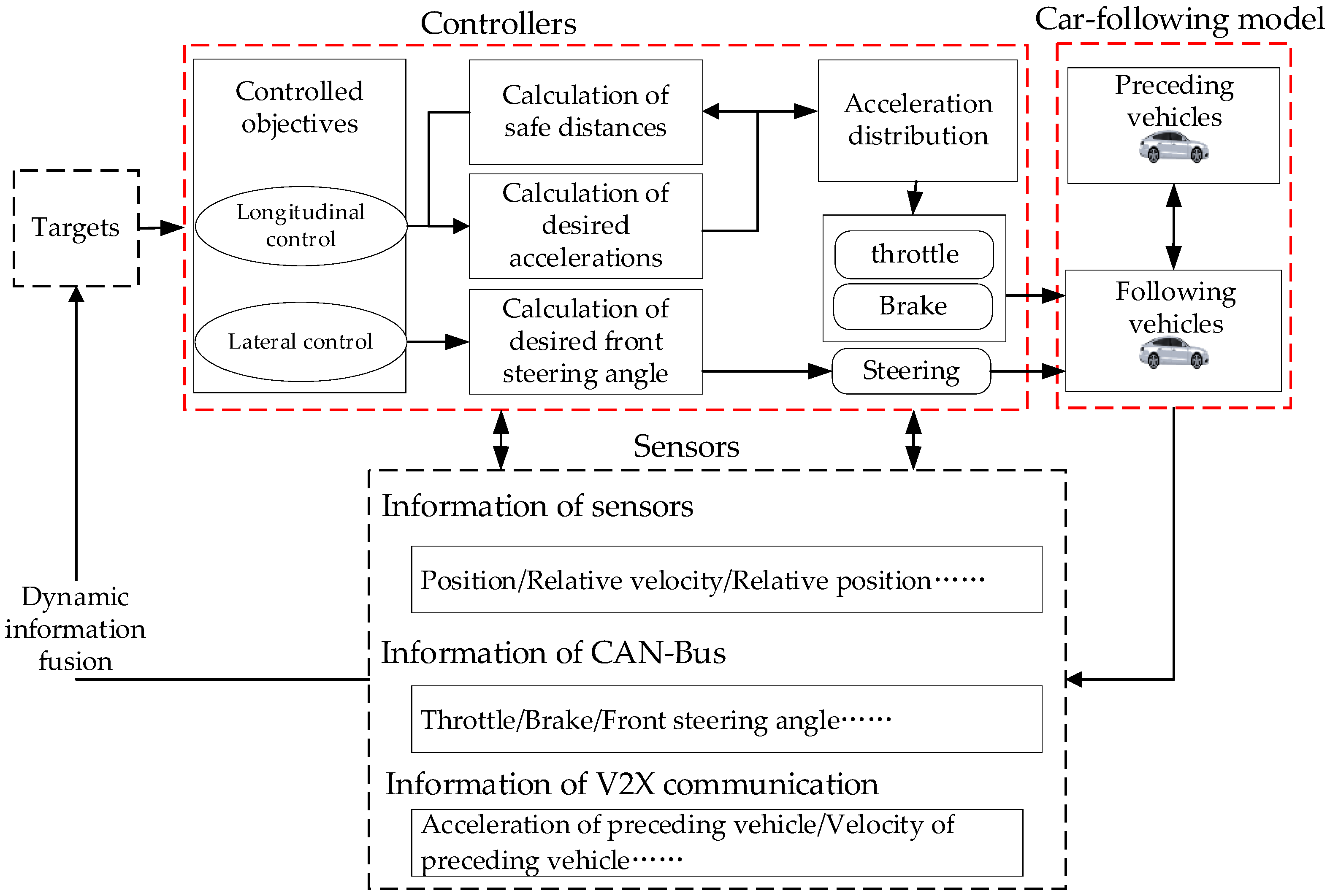
2.3. The Car-Following Model Based on Eco-Driving for ICVs

The decision layer is the core of the cooperative car-following system, where the eco-driving controller was designed for ICVs in the consideration of car-following behavior, fuel consumption, and emissions.

2.3.1. The Spacing Policy for ICVs

The car-following model focused on the influences between preceding vehicles and the following vehicle. When the velocity of the preceding vehicle changes, the velocity of the following vehicle needs to be changed simultaneously to ensure safety. The car-following model will be formulated based on the kinematics of vehicles and will further be quantitatively analyzed. Then, the optimal spacing between two vehicles and vehicular velocity will be achieved, accordingly. As shown in Figure 4, the vehicle $i$ is the preceding vehicle and the vehicle $i+1$ is the following vehicle. All vehicles in this model share state information through wireless communication.

Compared with the traditional constant safety (CS) spacing, the constant time headway (CTH) considers the relationship between the spacing of two vehicles and the real-time velocity. In this paper, the CTH is considered as the desired spacing between the preceding vehicle and the following vehicle. The desired spacing is expressed as Equation (1):

$$d_{\mathrm{tar}}\left(t\right)=d_0+hv\left(t\right)$$

(1)

where $d_0>0$ is the minimum safe spacing that needs to be maintained when two vehicles are standstill, $h>0$ is the time gap that needs to be maintained between two vehicles, and $v(t)$ represents the velocity of the vehicle at the moment $t$.

2.3.2. The Fuel Consumption and Emission Model for ICVs

A fuel consumption and emission model is very important for evaluating the effectiveness of the eco-driving controller, which can be estimated by velocity and acceleration [25] as in Equations (2) and (3):

$$C(t)=\alpha +{\beta }_1{P}_T(t)+{\left({\beta }_{2}m{a}^2(t)v(t)\right)}_{a>0}$$

(2)

$$P_T(t)=\max \{0,\hspace{0.33em}{d}_{1}v\left(t\right)+d_2{v}^2\left(t\right)+d_3{v}^3\left(t\right)+ma\left(t\right)v\left(t\right)\}$$

(3)

where $C(t)$ denotes the instantaneous fuel consumption, $\alpha$ stands for the idle fuel consumption, ${\beta }_1$ and ${\beta }_2$ are constant efficiency factors, $P_T(t)$ indicates the total power of the vehicle,$m$ is the mass of the vehicle,$d_1$, $d_2$ and $d_3$ are resistance coefficients, and $a(t)$ is the acceleration of the vehicle at the moment $t$.

The real-time emission rate of an ICV can be expressed by the measure of effectiveness (MOE) [26,27,28]. Ahn et al. [29] presented that the real-time MOE of a vehicle at moment $t$ is a function of the real-time velocity $v(t)$ and acceleration $a(t)$, which can be expressed as Equation (4):

$$\ln (MO{E}_e)={\displaystyle {\sum }_{i=0}^3{\displaystyle {\sum }_{j=0}^3(}}{K}_{i,j}^e\times v{(t)}^i\times a{(t)}^j)$$

(4)

where $MO{E}_e$ is real-time emission rate, $K_{i,j}^e$ represents the model regression coefficient for $MO{E}_e$, $i$ is the power exponent of velocity, and $j$ is the power exponent of acceleration.

2.3.3. The Eco-Driving Controller for ICVs

We define $\Delta r(t)$ and $\Delta v(t)$ as the current spacing and velocity difference between the i-th vehicle and its preceding vehicle; the formulation of the current spacing and velocity difference can be expressed as Equations (5) and (6):

$$\Delta r\left(t\right)=r^{i-1}\left(t\right)-r^i\left(t\right)$$

(5)

$$\Delta v\left(t\right)=v^{i-1}\left(t\right)-v^i\left(t\right)$$

(6)

where $r^i(t)$ and $r^{i-1}(t)$ represent the displacement of the i-th vehicle and its preceding vehicle, and $v^i(t)$ and $v^{i-1}(t)$ represent the velocity of the i-th vehicle and its preceding vehicle.

Then, the error $e_r(t)$ between the current spacing $\Delta r(t)$ and the desired spacing $d_{tar}(t)$ can be formulated as Equation (7):

$$e_r\left(t\right)=\Delta r\left(t\right)-d_{\mathrm{tar}}\left(t\right)$$

(7)

The velocity error $e_v(t)$ can be expressed as:

$$e_v\left(t\right)=\Delta v\left(t\right)$$

(8)

In this controller, lateral control should be considered when the vehicle drives in a curved road. We donate $v_y$ as the lateral velocity, $\dot{\phi }$ as the variation rate of yaw angle, $e_y$ as the lateral distance between the vehicle and the centerline, $e_{\phi }$ as the error of the yaw angle, $e_r$ as the spacing error, and $e_v$ as the velocity error. Besides, ${\delta }_f$ and $a^i$ represent the front steering angle and acceleration, respectively. $\rho$ and $a^{i-1}$ represent the road curvature and the acceleration of the preceding vehicle. $l_f$ and $l_r$ are the longitudinal distance from the center of gravity to the front and rear tires. $I_z$ denotes the yaw moment of inertia of the vehicle. $C_f$ and $C_r$ represent the tires cornering stiffness. $m$ is the mass of the vehicle, and $v_x$ refers to the longitudinal velocity. We define $x={\left[\begin{array}{llllll}{v}_y\hfill & \dot{\phi }\hfill & e_y\hfill & e_{\phi }\hfill & e_r\hfill & e_v\hfill \end{array}\right]}^T$; $u=\left[\begin{array}{c}{\delta }_f\\ a^i\end{array}\right]$; $d=\left[\begin{array}{c}\rho \\ a^{i-1}\end{array}\right]$. The model of the following vehicles can be expressed as:

$$\dot{x}=Ax+Bu+Wd$$

(9)

where $A=\left[\begin{array}{cccccc}\frac{C_f+C_r}{m{v}_x}& \frac{l_f{C}_f-l_r{C}_r}{m{v}_x}& 0& 0& 0& 0\\ \frac{l_f{C}_f-l_r{C}_r}{I_z{v}_x}& \frac{l_f{}^2{C}_f+l_r{}^2{C}_r}{I_z{v}_x}& 0& 0& 0& 0\\ 1& 0& 0& v_x& 0& 0\\ 0& 1& 0& 0& 0& 0\\ 0& 0& 0& 0& 0& 1\\ 0& 0& 0& 0& 0& 0\end{array}\right]$; $B=\left[\begin{array}{cc}-\frac{C_f}{m}& 0\\ -\frac{l_f{C}_f}{I_z}& 0\\ 0& 0\\ 0& 0\\ 0& -h\\ 0& -1\end{array}\right]$ and $W=\left[\begin{array}{cc}0& 0\\ 0& 0\\ 0& 0\\ -v_x& 0\\ 0& 0\\ 0& 1\end{array}\right]$. By discretizing Equation (9), the above model can be expressed by Equation (10) as:

$$x(k+1)=\overline{A}x(k)+\overline{B}u(k)+\overline{W}d(k)$$

(10)

where $\overline{A}=\left[\begin{array}{cccccc}\frac{\left(C_f+C_r\right)t_s}{m{v}_x}+1& \frac{\left(l_f{C}_f-l_r{C}_r\right)t_s}{m{v}_x}& 0& 0& 0& 0\\ \frac{\left(l_f{C}_f-l_r{C}_r\right)t_s}{I_z{v}_x}& \frac{\left(l_f^2{C}_f+l_r{}^2{C}_r\right)t_s}{I_z{v}_x}+1& 0& 0& 0& 0\\ t_s& 0& 1& v_x{t}_s& 0& 0\\ 0& t_s& 0& 1& 0& 0\\ 0& 0& 0& 0& 1& t_s\\ 0& 0& 0& 0& 0& 1\end{array}\right]$; $\overline{B}=\left[\begin{array}{cc}-\frac{C_f{t}_s}{m}& 0\\ -\frac{l_f{C}_f{t}_s}{I_z}& 0\\ 0& 0\\ 0& 0\\ 0& -h{t}_s\\ 0& -t_s\end{array}\right]$; $\overline{W}=\left[\begin{array}{cc}0& 0\\ 0& 0\\ 0& 0\\ -v_x{t}_s& 0\\ 0& 0\\ 0& t_s\end{array}\right]$; $t_s$ is the sampling interval.

Predictive state vectors and input vectors at the p-th step can be defined as:

$$X_k={\left[\begin{array}{cccc}x(k+1|k)& x(k+2|k)& \cdots & x(k+p|k)\end{array}\right]}^T$$

(11)

$$U_k={\left[\begin{array}{cccc}u(k|k)& u(k+1|k)& \cdots & u(k+p-1|k)\end{array}\right]}^T$$

(12)

$$D_k={\left[\begin{array}{cccc}d(k|k)& d(k+1|k)& \cdots & d(k+p-1|k)\end{array}\right]}^T$$

(13)

Therefore, according to Equation (10), the prediction state vector $X_k$ can be expressed as Equation (14):

$$X_k=\Psi x\left(k\right)+\Theta U_k+\Omega D_k$$

(14)

where $\Psi =\left[\begin{array}{c}\overline{A}\\ {\overline{A}}^2\\ ⋮\\ {\overline{A}}^p\end{array}\right]$,$\Theta =\left[\begin{array}{cccc}\overline{B}& \cdots & 0& 0\\ \overline{A}\overline{B}& \overline{B}& \cdots & 0\\ ⋮& ⋮& \ddots & ⋮\\ {\overline{A}}^{p-1}\overline{B}& {\overline{A}}^{p-2}\overline{B}& \cdots & \overline{B}\end{array}\right]$, and $\Omega =\left[\begin{array}{cccc}\overline{W}& \cdots & 0& 0\\ \overline{A}\overline{W}& \overline{W}& \cdots & 0\\ ⋮& ⋮& \ddots & ⋮\\ {\overline{A}}^{p-1}\overline{W}& {\overline{A}}^{p-2}\overline{W}& \cdots & \overline{W}\end{array}\right]$.

It has been noticed that one of the most effective ways to reduce fuel consumption is to reduce the acceleration of the vehicle, according to Equations (2) and (3). In order to optimize car-following behavior and reduce fuel consumption, we combined Equation (2) with Equation (14), and the object function can be formulated as

$$J=X_k^{T}P{X}_k+U_k^{T}Q{U}_k+R{\displaystyle {\int }_k^{k+p-1}C(t)} dt$$

(15)

where $P$ and $Q$ are the weight matrices, and $R$ is the weight factor.

In order to ensure safety, the vehicle was subject to the following velocity constraints as

$$v_{\min }\le v\left(t\right)\le v_{\max }$$

(16)

where $v_{\min }$ and $v_{\max }$ represent the minimum and maximum velocity of the vehicle during the process of driving.

Acceleration is related to the engine performance and is subject to the following constraints, which can be demonstrated as:

$$a_{\min }\le a\left(t\right)\le a_{\max }$$

(17)

where $a_{\min }$ represents the minimum acceleration of the vehicle during the process of driving, and $a_{\max }$ represents the maximum acceleration of multiple preceding vehicles during the process of driving.

Moreover, the error between vehicular spacing and desired spacing should be subject to the following constraints:

$$0\le e_r\left(t\right)\le e_{r,\max }$$

(18)

$$\underset{t\to \infty }{lim}{e}_r\left(t\right)=0$$

(19)

where $e_{r,\max }$ is set up as the max error between vehicular spacing and desired spacing.

Therefore, the control quantity can be concluded as the following problem:

$$\begin{array}{l}\mathrm{Min}\hspace{0.33em}J=X_k^{T}P{X}_k+U_k^{T}Q{U}_k+R{\displaystyle {\int }_k^{k+p-1}C(t)} dt\\ s.t.v_{\min }\le v\left(t\right)\le v_{\max }\\ a_{\min }\le a\left(t\right)\le a_{\max }\\ 0\le e_r\left(t\right)\le e_{r,\max }\\ \underset{t\to \infty }{lim}{e}_r\left(t\right)=0\end{array}$$

(20)

The first two terms ($X_k^{T}P{X}_k+U_k^{T}Q{U}_k$) in Equation (20) were used to optimize car-following behavior. The third term ($R{\displaystyle {\int }_k^{k+p-1}C(t)} dt$) in Equation (20) was used to constrain fuel consumption. In order to minimize the objective function $J$, the controller calculated the acceleration and front steering angle of the vehicle.

3. Co-Simulation Platform Design for ICVs Based on ROS/PreScan

3.1. Structure of the Co-Simulation Platform

PreScan is a physics-based simulation platform used for the development of vehicular dynamic systems with building traffic scenarios, simulating road environments, and further controlling vehicular driving states. It has been extensively used because of the intuitive simulation results provided for vehicle controllers. ROS is a software architecture used to develop robot programs.

Due to the high cost and risk of real vehicle experiments, a hardware-in-loop (HIL) experimental platform was established based on PreScan and ROS in our paper. In this platform, the control parameters of each vehicle can be evaluated by PreScan and then be transferred to ROS. After that, the received command was executed in ROS. A HIL simulation environment was be established with the above experimental platform to verify the proposed eco-driving controller. The construction of the simulation environment is shown as Figure 5.

3.2. Nodes Design for ICVs Based on ROS

In this paper, ROS was used to design the program of the cooperative driving vehicle with the advantages of modular programming and distributed computing. In ROS, the program codes are stored and operated at nodes. Topics are named buses for nodes to exchange information. Each node runs independently and delivers information through publishing and subscribing topics.

The vehicle control nodes of ROS are shown in Figure 6, where each vehicle obtained data through node /receive_data which mainly includes time and control parameters. After being processed by node /receive_data, the data was published through topic /cmd_vel. The subscribers of node /throttle_control and /brake_control executed the commands through the topic /cmd_vel to control the vehicle. Vehicular sensors mainly included millimeter wave radar and status sensor, where node /radar can obtain the spacing from the preceding vehicle, and node /self can obtain the velocity, acceleration, and other information of the vehicle.

4. Experimental Results and Discussion

There was a 2-km road section in this experiment. As shown in Figure 7, a platoon consisting of a leading vehicle and two following vehicles was applied in each group of experiments. The change of the spacing between any of two following vehicles can be observed from the top view.

In this scenario, we selected road curvature, vehicular velocity, and spacing, which are critical parameters as the inputs of the eco-driving controller. The desired acceleration and the desired front steering angle of each connected vehicle were defined as outputs. Besides, a set of information containing acceleration, velocity, position, fuel consumption, and carbon dioxide emissions were selected as the main indexes. Among them, the acceleration, velocity, and position were obtained from the ROS, and the fuel consumption and carbon dioxide emissions were calculated by Equations (2)–(4). In order to verify the effectiveness of the proposed controller, a strategy for the control of a standard MPC was proposed and developed. In addition, we considered the eco-driving constraints in the controller, and the improved MPC strategy was re-developed with the objective of being environmentally sustainable. The working procedure of the improved MPC strategy is shown in Figure 8. In the HIL simulation experiments, the emission coefficient of carbon dioxide was used to value the MOE [30], shown in

Table 2. The emission coefficients for the MOE of carbon dioxide [30].

${\mathit{K}}_{\mathit{i},\mathit{j}}^{\mathit{e}}$	$\mathit{a}(\mathit{t})\ge 0$				$\mathit{a}(\mathit{t})<0$
(mg/s)	$\mathit{j}=0$	$\mathit{j}=1$	$\mathit{j}=2$	$\mathit{j}=3$	$\mathit{j}=0$	$\mathit{j}=1$	$\mathit{j}=2$	$\mathit{j}=3$
$i=0$	−7.735	0.2295	−5.61 × 10−3	9.773 × 10−5	−7.735	−0.01799	−4.27 × 10−3	1.8829 × 10−4
$i=1$	0.02799	0.0068	−7.722 × 10−4	8.38 × 10−6	0.02804	7.72 × 10−3	8.375 × 10−4	3.387 × 10−5
$i=2$	−2.228 × 10−4	−4.402 × 10−5	7.90 × 10−7	8.17 × 10−7	−2.199 × 10−4	−5.219 × 10−5	−7.44 × 10−6	2.77 × 10−7
$i=3$	1.09 × 10−6	4.80 × 10−8	3.27 × 10−8	−7.79 × 10−9	1.08 × 10−6	2.47 × 10−7	4.87 × 10−8	3.79 × 10−10

. The parameters defined in Equations (2) and (3) in this paper are set up as

Table 3. Parameters related to fuel consumption.

Parameters	Values	Units
$\alpha$	0.666	mL/s
${\beta }_1$	0.072	/
${\beta }_2$	0.0344	/
$m$	1680	kg
$d_1$	0.269	/
$d_2$	0.0171	/
$d_3$	0.000672	/

.

The parameters of the eco-driving controller of ICVs are displayed in

Table 4. Parameter settings of the model predictive control strategy.

Parameters	Values	Units
$v_{\min }$	15	m/s
$v_{\max }$	30	m/s
$a_{\min }$	−3	m/s${}^2$
$a_{\max }$	3	m/s${}^2$
$e_{r,\max }$	2	m
$p$	10	ms
$c$	1	ms
$s$	100	ms

, where $p$ is the prediction horizon, $c$ is the control horizon, and $s$ is the control period. The velocity of the vehicle fell in [15, 30] m/s, and the acceleration was set up as [−3, 3] m/s${}^2$. In addition, the initial states of vehicles are shown in

Table 5. Initial states of ICVs.

Initial State	Units	Preceding Vehicle	Following Vehicle 1	Following Vehicle 2
Position	m	50	25	0
Velocity	m/s	10	10	10
Space	m	0	25	25

.

There were two experimental scenarios with constant acceleration and variable velocity involved in the HIL simulation experiments.

Scenario 1: Constant acceleration of the preceding vehicle.

In this scenario, the preceding vehicle drives with the acceleration of 1 m/s${}^2$. Once its velocity reaches 30 m/s, the vehicle will keep moving at a constant velocity. The real-time states are shown as Figure 9, Figure 10, Figure 11, Figure 12, Figure 13, Figure 14, Figure 15 and Figure 16.

From Figure 9, Figure 10, Figure 11 and Figure 12, the velocities and accelerations of vehicle 2 and vehicle 3 were compared with the standard and the improved MPC strategies. The velocity was gradually adjusted to 30 m/s after 30 s, and the accelerations were stable at 0. However, vehicle 2 and vehicle 3 showed their deceleration at the beginning of the standard MPC strategy. When vehicle 1 accelerated, the acceleration of the following vehicle under the improved MPC strategy was very small, which facilitated the convergence rate of the acceleration. In the same state of vehicle 1, the fluctuations in the accelerations of the following vehicles occurred under the standard MPC between 10 s and 20 s, which was caused by the acceleration at 10 s. As shown in Figure 12, after vehicle 1 suddenly accelerated, the maximum acceleration of vehicle 2 could be up to 1.7 m/s${}^2$, which reflects the moderate acceleration control of the improved MPC strategy. The accelerations in Figure 11 and Figure 12 reflect that the change rate of acceleration of the standard MPC strategy is greater than that in the improved MPC strategy, which affects the fuel consumption and emissions of the vehicle. In addition, it can be seen from the maximum acceleration in these two figures that the improved MPC strategy was more adaptable to constraints compared to the standard MPC strategy.

Figure 13 and Figure 14 compare the movements of vehicle 2 and vehicle 3. The trends show that they were consistent with the movement of vehicle 1 under the two car-following strategies. As the velocity increased, the spacing between vehicle 1 and vehicle 2 increased, which was in line with the spacing caused by the CTH strategy. There was no intersection in position in these two figures, which indicates that there was no collision between any of the two vehicles.

The fuel consumption and carbon dioxide emissions under the two car-following are shown in Figure 15 and Figure 16. The vehicles consumed more fuel and emitted more carbon dioxide when accelerating. After 10 s, the fuel consumption and carbon dioxide emissions in the standard MPC strategy were more than that in the improved MPC strategy, which were caused by the acceleration fluctuations of the vehicles in the standard MPC strategy. The total fuel consumption with the improved MPC strategy was 0.4393 L at 80 s, which was about 3.71% less than that with the standard MPC strategy. As shown in Figure 16, compared to the standard MPC strategy, the total carbon dioxide emissions under the improved MPC strategy were reduced by 4.32%.

Scenario 2: Variable velocity of the preceding vehicle.

In a cooperative car-following model, the preceding vehicle may adjust its velocity according to the road state and the signal state. The scenario of vehicles with varying velocities was designed and the extensive experiments were conducted. In order to test the car-following behaviors and fuel consumption, the preceding vehicle will run at a variable velocity from 15 to 32.5 m/s.

From Figure 17, Figure 18, Figure 19 and Figure 20, we can see that the velocity and acceleration of the following vehicle changed with the preceding vehicle under two car-following strategies. It was shown that the trends of these two vehicles were the same, but the decelerations of vehicle 2 and vehicle 3 were displayed at the beginning of the standard MPC strategy, which is shown in Figure 17. The minimum velocity of the standard MPC strategy was 13.7 m/s, and the maximum velocity was 34 m/s, while the minimum velocity with the improved MPC strategy was 15 m/s and the maximum velocity was 32.7 m/s. Therefore, the improved MPC strategy had superiority in velocity control. With the same state of the preceding vehicle, the accelerations of the following vehicle vibrated more frequently along with the change of velocity under the standard MPC strategy, which was unexpected to the control of the vehicle.

The higher fuel conservation and lower carbon dioxide emissions can be produced by the improved MPC strategy by predicting the running state of the preceding vehicle and executing a smaller acceleration. As shown in Figure 20, although the velocity of the preceding vehicle changed frequently, the acceleration of the following vehicle changed relatively moderately, which indicates that the improved MPC strategy achieved relatively stable control of the following vehicle.

Figure 21 and Figure 22 demonstrate that the movements of the following vehicles were consistent with the trend of the preceding vehicle under two car-following strategies. According to the CTH strategies, the spacing between the preceding vehicle and the following vehicles increased along with the velocity. There was not any intersection in these three lines in position, which indicates that there was no collision between any of the two vehicles. From Figure 19 and Figure 20, we can see that the maximum value of acceleration of the following vehicles was 3.4 m/s${}^2$ under the standard MPC strategy and 2 m/s${}^2$ under the improved MPC strategy, which demonstrates that the improved MPC strategy can effectively avoid rapid acceleration.

Figure 23 and Figure 24 show the performances of fuel consumption and carbon dioxide emissions under two car-following strategies. It was evident that the vehicles consumed more fuel and emitted more carbon dioxide when accelerating, while the improved MPC strategy reduced some unnecessary acceleration processes and reduced fuel consumption and emissions. According to Figure 23, the total fuel consumption under the improved MPC was 0.37351 L at 80 s, which was about 6.77% less than that in the standard MPC strategy. As shown in Figure 24, the carbon dioxide emissions under the improved MPC strategy were reduced by 7.91% by comparing them with the standard MPC strategy, which proves the effectiveness of the improved MPC strategy.

To evaluate the accuracy of the simulation results, we conducted 10 experiments in each of the two scenarios and recorded the total fuel consumption for 80 s, as shown in

Table 6. Total fuel consumption of 10 experiments (liter).

		1	2	3	4	5	6	7	8	9	10
Scenario 1	MPC	0.45623	0.45622	0.45623	0.45621	0.45624	0.45620	0.45625	0.45623	0.45622	0.45623
	Improved MPC	0.43930	0.43931	0.43931	0.43928	0.43929	0.43930	0.43932	0.43931	0.43933	0.43930
Scenario 2	MPC	0.40063	0.40061	0.40064	0.40063	0.40062	0.40063	0.40061	0.40060	0.40065	0.40063
	Improved MPC	0.37351	0.37348	0.37350	0.37353	0.37351	0.37349	0.37351	0.37350	0.37353	0.37349

.

Based on the data in Table 6, we could calculate the confidence intervals for the strategies in the two scenarios. In Scenario 1, the confidence intervals for the standard MPC strategy and the improved MPC strategy at the confidence level of 95% were 0.400625 ± 0.0000089 and 0.373505 ± 0.0000097, respectively. In Scenario 2, the confidence intervals for the standard MPC strategy and the improved MPC strategy at the confidence level of 95% were 0.456226 ± 0.0000084 and 0.439305 ± 0.0000084, respectively. Therefore, the accuracy of the simulation results can be guaranteed.

5. Conclusions

In this paper, we proposed an eco-driving controller based on the characteristics of the vehicular dynamics system for ICVs. The proposed controller employed the improved MPC strategy to optimize the acceleration of the following vehicle, while reducing fuel consumption and carbon dioxide emissions and simultaneously ensuring the safety of the following vehicle. The effectiveness of the eco-driving controller was also verified through a co-simulation platform composed of ROS and PreScan software. The final experimental results showed that the proposed controller can reduce fuel consumption by 3.71% and reduce carbon dioxide emissions by 3.42% in the scenario of a preceding vehicle with constant velocity. In the scenario of a preceding vehicle with variable velocity, the proposed controller can reduce fuel consumption by 6.77% and reduce carbon dioxide emissions by 7.91%.

The control of the proposed eco-driving controller may be affected if conventional vehicles are involved in the ICVs. In order to explore the effective solutions to this scenario, we consider developing an improved eco-driving controller by taking the impact of vehicle diversity into consideration in the future. In addition, we will study the impact of lateral control on fuel consumption and emissions and introduce lane-changing scenarios into the simulation.