Modelling and Parametric Analysis of a Brine Treatment Unit Using a High-Temperature Heat Pump and a Vacuum Evaporator

Abstract

The brine produced from desalination systems is a highly concentrated mixture, including cleansing chemicals from the water treatment processes that can possibly degrade ecosystems in discharge areas. Evaporation is a widely used method for the treatment of high salinity mixtures; however, it requires careful monitoring of the temperature and pressure in order to protect the equipment from the highly corrosive environment of the brine discharge. The proposed brine treatment system is based on the principle of vacuum evaporation with the use of a high-temperature heat pump, which is classified as “green technology”. In this study, a thermodynamic analysis of a vacuum evaporation system with a nominal freshwater production capacity of 160 L/h has been carried out, employing a numerical tool to model the flash evaporator and the heat pump. The analysis focuses on the parameters that present the most significant impact on the system’s efficiency and water production, such as the recirculation ratio, the set-point temperature of the heat pump and the pressure difference provided by the vacuum pump. The results show that, for the constant vacuum pressure difference, the water production increases with the increase in the set-point temperature and the recirculation ratio, but leads to the reduced COP of the heat pump and to an elevated specific energy consumption. Moreover, it is shown that an increased vacuum pressure difference leads to increased water production, but reduces the COP. Finally, the minimum specific energy consumption of 150 kWh/m³ of produced freshwater can be achieved for a set-point at 75 °C and vacuum of 0.21 bar, leading to a levelized cost of water about 11 €/m³.

1. Introduction

The continuous global population increase has created the necessity of intensive water consumption in the human environment. Although 70% of the earth is water-covered, only 2.5% of it is freshwater, only 1% is easily accessible and overall, only 0.007% of the planet’s water is available to fuel and feed its 7.9 billion people. Therefore, water treatment systems emerge as a necessary solution to the water scarcity problem. Reverse osmosis (RO) has become dominant technology nowadays, since the required specific energy consumption (kWh/m³ produced freshwater) is reduced compared to the thermal technologies. To that end, the incorporation of very efficient energy recovery systems and the evolution of membrane technology play a key role.

Nevertheless, reverse osmosis desalination technology remains an energy-cost intensive water treatment process, with serious environmental impacts. In addition to the contribution of desalination to GHGs emissions, a significant environmental burden is incurred, due to the rejection in the oceans and soil of the high concentration saline solution (brine), as a by-product of the process. This results in soil, aquifer and marine ecosystems degradation. From these technologies, MSF is widely used for brine treatment towards a MLD/ZLD approach, even if it was first developed for seawater desalination treatment. This technology incorporates the heating of brine and its instantaneous pressure drop, forcing it to almost flash into steam [1]. The rest of the brine stream moves on to the next stage to become steam in even lower pressures and the cycle goes on. Freshwater is produced by steam condensation with the use of the cool brine stream. An MSF assembly can usually include up to 30 stages depending on the brine load and salinity, while the maximum capacity of freshwater production can reach 75,000 m³/d. MSF requires minimum pretreatment and shows low fouling potential [2]; however, it exhibits high electricity consumption (3.5–5 kWh_e/m³) and high thermal energy consumption (up to 83.3 kW_th/m³ for stand-alone systems and up to 47.2 kW_th/m³ considering co-generation) [3]. On the other side, a variant of the MSF called vacuum membrane distillation (VMD) is one of the most favorable MD configurations [4]. In VMD, the vapor is isolated with the exercise of a vacuum pressure to the permeate flow side of the membrane, which is maintained at just lower than the saturation pressure of volatile components in the hot feed flow. The membrane is kept between the hot feed flow stream and a vacuum space, while vapor is selected in an external condenser, outside of the membrane module [5]. The vacuum on the permeate flow stream permits a higher partial pressure gradient, leading to an additional driving force for the process, and thus a higher permeate production rate compared to other membrane distillation (MD) configurations [6,7]. Another benefit of the use of VMD is the fact that a vacuum leads to negligible heat loss by conduction. However, it should be highlighted that additional electrical power is needed due to the vacuum pump use [8].

In industrial applications, a simplified configuration of VMD is usually used for oil or other substance refinery [9,10]. It is simply called vacuum distillation and it is a preferred solution when elements that decompose when heated in atmospheric pressure, or have high boiling points that would increase the heating system requirements, are involved. The process is similar to VMD; the pressure is lowered in a column above the solvent to less than the vapor pressure of the mixture in discussion, creating a vacuum and evaporating the substances with lower vapor pressures. With the decrease in the pressure below atmospheric, the temperature demand for the evaporation of the distillate decreases as well, resulting in an overall heating requirement decrease for the system. Vacuum distillation is also used in large industrial plants for seawater desalination. The seawater is put under vacuum pressure in a column to lower its boiling point and with the application of heat, the permeate is distilled and condensed in an external condenser. Thus, the process runs continuously without the loss of vacuum pressure. The condensation heat removal is realized in a sink using the feed seawater to cool it down and preheat the seawater stream. In some cases, instead of condensers, pumps are used to mechanically compress vapor, acting as heat pumps, concentrating the heat from the vapor and allowing it to be returned and reused by the feed seawater [11,12].

Extended research has been conducted in the field of MSF and MEE systems simulation for brine treatment and ZLD technologies. Ogosu et al. [13] have developed a steady-state simulation model for a multiple-effect evaporator for application in the caustic soda industry. The model describes mass and energy balance equations, as well as heat transfer rate equations, for all the components and results in steam economy, improving up to 2.46 at evaporator inlet temperatures of 90 and 76 °C for the first and second effect. Nafey et al. [14] have designed a multiple-effect evaporator desalination process with different configurations using a Matlab model. Their results verified the development of a very accurate model (maximum relative error ~0.7%) for MEE processes, including a large matrix solved for temperatures and flow rates of brine and vapor for all the units in any given configuration, such as forward, backward, parallel and mixed plants. In MSF technology, several simulation models have been developed and applied for optimal operation in desalination systems [15,16,17], including daily operational cost optimization, design (number of stages) and operation (rejected seawater and brine recycle flowrate) optimization and daily productivity optimization. A spray flash evaporation system, combined with a hybrid latent heat storage technology in order to develop an energy-saving desalination system that stores intermittent thermal energy, such as waste heat, solar heat or heat from the surplus steam of a power station, at night and utilizes the stored energy not only for the generation of process steam from seawater for industries and domestic air conditioning but also for the production of freshwater from the generated steam for industrial and domestic uses on-demand, has also been developed and evaluated by Miyatake et al. [18]. Their research resulted in more than 95% usage of the amount of stored energy for process steam and freshwater production, confirming a high efficiency system. Vakilabadi et al. [19] have conducted an energy and exergy analysis and performance evaluation of a vacuum evaporator for solar thermal power plant MLD systems. In their research, the effect of the dimensional and operating parameters on the freshwater flow rate, exergy efficiency and power consumption were investigated, concluding that the amount of produced freshwater flow rate is independent of the recirculating flow rate and is a function of the evaporator’s volume. Another result of their investigation was that, with the brine concentration increase, a decrease in the produced freshwater flow rate and in the total power consumption was noticed and that the increase in the volume of the vacuum evaporator led to a freshwater flow rate increase. Finally, Panagopoulos [20] presented a techno-economic evaluation of a ZLD system, using multi-effect distillation with thermal vapor compression operating at 120 °C, simulating the system and estimating a freshwater cost of about 4 US$/m³.

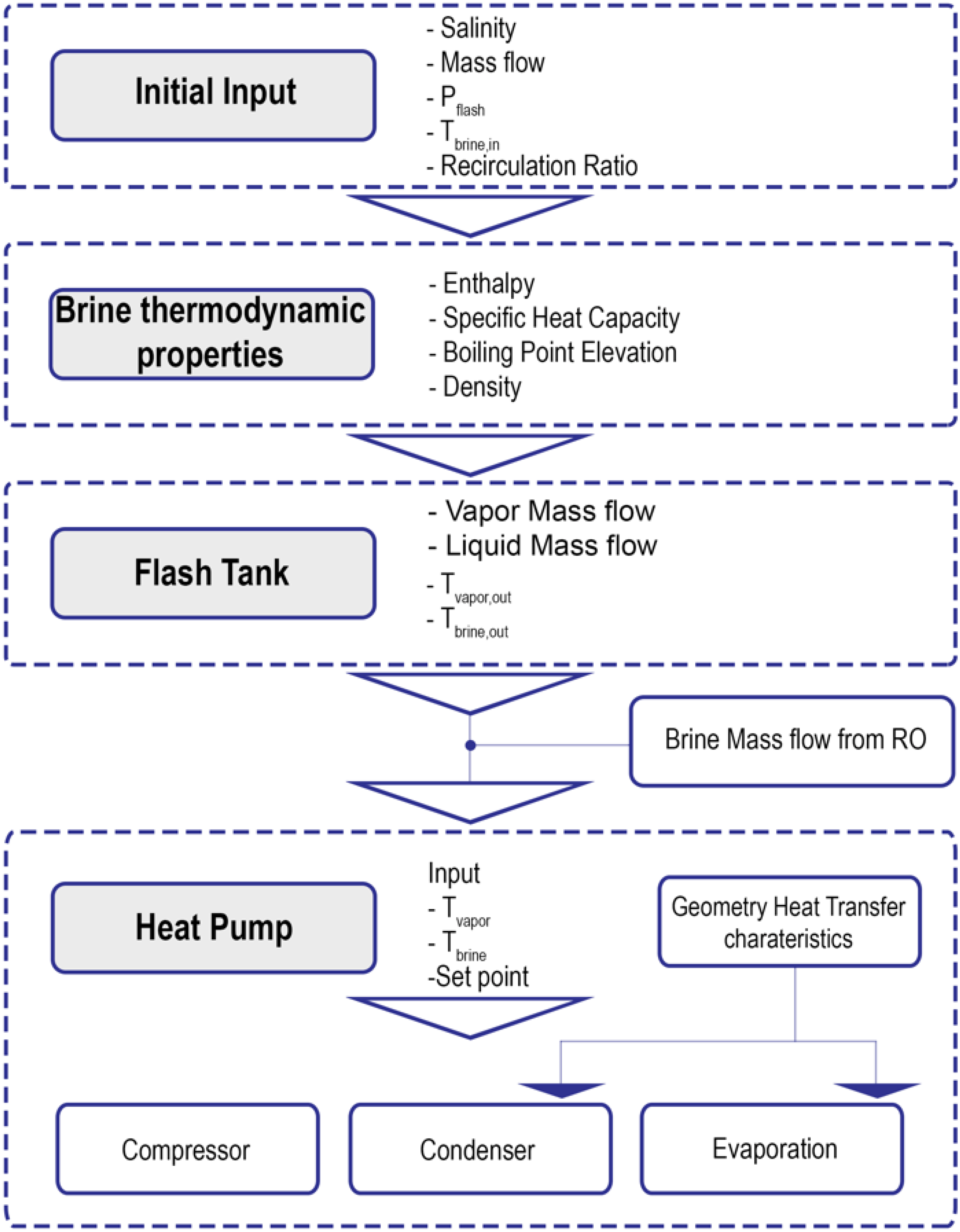
As noticed in the international literature, most of the research concentrates on the VMD and vacuum distillation systems coupled with solar or geothermal heat sources, while the use of the heat pump as a heat source remains relatively unexplored. The current research attempts to combine high-efficiency and eco-friendly technologies for brine treatment in order to enhance the freshwater production and eliminate the environmental and cost impact because of the brine rejection, which could be applied in small islands with limited habitants and varying demand in winter and summer. The innovation of the proposed system consists of the heating of the brine before it enters the flash tank, taking advantage of the rejected heat for the condensation of the refrigerant on the HP side, and in parallel, the system makes use of the latent enthalpy of the vapor that flows out of the flash tank, evaporating the refrigerant of the heat pump. More specifically, the combination of a high-temperature heat pump (HTHP) with a brine treatment technology based on evaporation under a vacuum is investigated, focusing on the parameters affecting the freshwater production and the electrical energy consumption. A heat pump system that is designed to reach a COP of up to 3.7, as a renewable energy technology, in principle, acts as the energy prime mover that is capable of mitigating the GHG impact of the energy intensive brine treatment process. The goal is to make the selected brine treatment system environmentally friendly but also cost-effective to a great extent. However, the proposed combined HTHP-brine treatment process entails an in-depth analysis and optimization, since it constitutes a sensitive, multi-parametric study that involves several variables, such as vacuum pressure, evaporation temperature, recirculation ratio, brine concentration etc.

2. System Description and Modelling

2.1. System Description

In this study, a mathematical modelling was elaborated and an energy analysis of the minimum liquid discharge (ΜLD) system for recovering freshwater from the brine was performed. A schematic diagram of the system is shown in Figure 1. The system is fed with brine water with a salinity in the order of 69,000 ppm. This brine concentration is typical of an RO unit with a recovery ratio of 40% supposed to treat seawater of 42,000 ppm and was calculated using ROSA software [21].

The integrated brine treatment system consists of a heat pump and a flash evaporation tank. The brine from RO is led to the condenser of the heat pump (1–2), where its temperature rises up to 80 °C, before it is driven to the flash tank, using a recirculating pump (2–3). The flash tank is under a pressure difference of 0.7–0.8 barg compared to the atmospheric one, which is continually preserved by a suitable vacuum pump. When the brine at this temperature enters the flash tank, its pressure is decreased to the pressure of the tank. At this point, the brine is superheated in relation to the saturation temperature that corresponds to the flash tank pressure, while this abrupt depressurization of the feed liquid brine, in conjunction with the superheat of the brine, lead to a phase change in the liquid; thus, a fraction of its mass is vaporized. The void fraction development depends on this depressurization and the superheating, making the brine inlet temperature and the vacuum in the tank the decisive parameters for the fraction that is vaporized [22,23]. Figure 2 illustrates the process using a pressure-composition diagram under a constant flash temperature. Therefore, the fluid is separated into a vapor and a liquid phase. The vapor is taken off from the upper part of the tank, while the liquid drains to the bottom of the tank. The vapor produced under these conditions flows out of the tank (3–4i) towards the heat pump’s evaporator, where it is condensed by dissipating its enthalpy (4i–5). On the other hand, the liquid fraction of the process remains as brine with increased salinity and also flows out of the tank (3–4ii). When the brine exits the flash tank, a fraction of the brine is rejected to the sea, while the rest flows back to the brine heater (4ii–1) and the amount of the rejected brine is balanced with the brine coming from the RO unit. Therefore, a large percentage of the brine with increased salinity recirculates, is heated up in the condenser and treated in the flash evaporation tank. The vapor is then driven to the heat pump’s evaporator, which extracts the heat from the vapor that condensates (4i–5). The recovered freshwater is finally collected in a tank (5–6).

The heat pump is used to supply heat to the brine, but also to condensate the vapor as it exits the flash tank. The operation of the heat pump is roughly described as follows: the refrigerant is compressed through a semi-hermetic screw compressor (R1–R2) and then, it is cooled to the unit’s condenser by dissipating its heat to the brine (R2–R3). The subcooled fluid passes through a filter before it is expanded through an electronic expansion valve (R3–R4) and finally, it is heated through an evaporator to superheated vapor (R3–R4).

For the modelling, R134a is selected as the working refrigerant of the heat pump as it is suitable for this temperature range, although a fourth generation substitute, such as R1234ze(E), of ultra-low GWP could be preferably chosen for environmental purposes. However, the performance variables (i.e., power consumption and mass flow rate as a function of evaporation and condensation temperature) of the commercially available compressor that has been chosen are provided only by the manufacturer for R134a (see Section 2.2.2). The accuracy in the calculation of the performance of the compressor at varied conditions can be only assured if these variables are provided by the manufacturer.

2.2. Mathematical Modelling

This study employs a numerical tool developed with the use of Matlab Simscape [24], which includes block-components that are built by specified thermodynamic equations, mass and energy equilibria to describe each process of the system. Each block of the developed model represents one of the following components of the system: the heat pump’s components (compressor, condenser, expansion valve, evaporator, receiver) and the flash tank with the appropriate recirculation and vacuum pumps. The properties of the brine, such as density, boiling point elevation, specific heat capacity or enthalpy, are calculated according to the MIT model [25,26] and are based on the salinity, while the thermodynamic properties of R134a are calculated from the CoolProp library [27]. It must be noted that the MIT model has been elaborated for salinity up to 12%.

The performance of the heat pump under varying conditions is calculated by a physics-based model. Each component is calculated separately and then linked with the next component through the input parameters, while conservation equations of heat and mass transfer are applied. The following assumptions were considered to develop the mathematical model:

• The components are considered to be well insulated, so heat loss to the surroundings is neglected (adiabatic).
• The model is considered quasi-steady.
• Expansion and compression processes are assumed to be adiabatic.

As was described above, the brine that flows out of the flash tank has an increased salinity compared with the feed brine. The part of the brine that is not rejected recirculates towards the brine heat, while the rejected brine is balanced with the amount of brine coming from RO and the whole flow re-enters the flash tank. Therefore, there is only a fraction of the feed brine that recirculates at a temperature equal to the flash tank temperature, while the brine coming from RO is still cold, since it has not passed from the brine heater, which is the condenser of the heat pump. Depending on the fraction of the initial brine that recirculates, the required thermal load to heat the whole brine at the desired temperature (setpoint of the heat pump) varies. Thus, the recirculation ratio $\left(r\right)$ is considered to define the part of the brine that recirculates ${\dot{m}}_{b, rec}$ (kg/s) over the initial total brine, ${\dot{m}}_{b, ini}$, (kg/s), which is as follows:

$$r=\frac{{\dot{m}}_{b, rec}}{{\dot{m}}_{b, ini}}$$

(1)

The recirculation ratio has values between 0 and 1 or can be presented as a percentage. Figure 3 presents the flowchart of the numerical process for the developed model, which is discussed in the following section.

2.2.1. Flash Tank

The flash tank is modeled by a custom Simscape block. The mass and energy equilibria are expressed assuming that the feed brine enters the flash tank, while the vapor and the liquid phases flow out of this, with the corresponding specific enthalpy in the following equations:

$${\displaystyle \sum }_{i=1}^N{\dot{m}}_o={\displaystyle \sum }_{i=1}^N{\dot{m}}_{in}$$

(2)

$$\frac{\partial Q}{\partial t}-\frac{\partial W}{\partial t}={\displaystyle \sum }_{i=1}^N{\dot{m}}_o{h}_o-{\displaystyle \sum }_{i=1}^N{\dot{m}}_{in}{h}_{in}$$

(3)

$$\frac{{\dot{m}}_{vap}}{{\dot{m}}_{b, total}}=\frac{h_{brine, in}-h_{liq,sat}}{h_{vap, sat}-h_{liq,sat}}$$

(4)

where ${\dot{m}}_{in}$ and ${\dot{m}}_o$ are the mass flow rates that flow into and out of the tank in kg/s, respectively, i the number of components at the inlet and outlet of the tank, $Q$ the heat provided to the flash tank (if adiabatic $Q=0$), $W$ is the work consumed in the tank (zero in this case) and $h_{in}$ and $h_o$ are the specific enthalpies of the inlet and outlet streams, respectively, in kJ/kgK. The specific enthalpy and other thermodynamic properties of the feed brine and the pressure in the flash tank are considered as inputs for the model. Applying the energy equilibrium, the outlet sp. enthalpy for the vapor and liquid parts of the flow and their respective fractions are estimated, according to Equation (4). In this equation, ${\dot{m}}_{vap}$ and ${\dot{m}}_{b, total}$ are the mass flow of the generated vapor and the total brine at the inlet of the flash in kg/s, respectively, $h_{brine, in}$ is the specific enthlapy (kJ/kg) of the inlet brine coming from the brine heater, $h_{vap, sat}$ is the specific enthalpy of the saturated vapor (kJ/kg) at the flash tank pressure, and $h_{liq,sat}$ is the specific enthalpy of the saturated liquid brine (kJ/kg), based on the brine salinity. The performance of the flash evaporator was validated with the results presented by the experimental study of Miyatake et al. [18] for the superheat of the inlet brine more than 10 K, compared to the flash evaporator saturation temperature (as function of pressure).

2.2.2. The Heat Pump Model

i.

Compressor

The compressor of the HTHP system is selected to be of a screw type (Hanbell RC2-100G) [28], with a displacement of 98 m³/h at 2950 rpm and a volume ratio of 3.0. The compressor model in Simscape uses as input the evaporation, condensation and ambient temperature. As the compressor manufacturer provides information about the mass flow and power coefficients (

Table 1. Power consumption and mass flow rate coefficients given by Hanbell for the RC2-100G compressor model.

Coefficient	For Power Consumption Estimation	For Mass Flow Rate Estimation
$c_1$	−41,051	4527.2
$c_2$	733.81	49.7467
$c_3$	1935.7	−145.1809
$c_4$	14.075	−0.18796
$c_5$	−25.59	0.26831
$c_6$	−20.338	2.06611
$c_7$	0.0261	0.019067
$c_8$	−0.2159	−0.003456
$c_9$	0.237	−0.001059
$c_{10}$	0.0929	−0.010284

) through the polynomial $y$ below for R134a, the mass flow rate and the power consumption are estimated as a function of the evaporation and condensation temperatures, ($T_{ev}, T_{cd}$). The mass flow rate in kg/h and the power consumption in W are calculated using the following equation with the respective coefficients from Table 1:

$$y=c_1+c_2\times T_{ev}+c_3\times T_{cd}+c_4\times {T_{ev}}^2+c_5\times T_{ev}\times T_{cd}+c_6\times {T_{cd}}^2+c_7\times {T_{ev}}^3+c_8\times T_{cd}\times {T_{ev}}^2+c_9\times T_{ev}\times {T_{cd}}^2+c_{10}\times {T_{cd}}^3$$

(5)

ii.

Condenser

The condenser of the heat pump is modeled as a shell and tube heat exchanger using the condenser-evaporator (TL-MA) block model, where energy is transferred from the refrigerant to the colder brine and various parameters, such as flow arrangement (counter flow) and geometrical characteristics and is set to reflect the problem specifications. Heat transfer between the hot side (refrigerant) and cold side (brine) is calculated based on the effectiveness-number of transfer units (ε-NTU) method for the counter-flow heat exchanger. The heat transfer is divided into three zones (liquid, mixture and vapor) and the heat transfer is calculated for each phase. The heat transfer calculation is based on the Gnielinski correlation for the subcooled liquid or superheated vapor zones, while the Cavallini–Zecchin correlation is used for the liquid–vapor mixture zone. The heat transfer characteristics of the condenser are summarized in

Table 2. Geometric characteristics of the heat pump’s evaporator and condenser.

Parameter	HTHP Condenser	HTHP Evaporator
Heat transfer coef. (W/m2K)	1530	306
Heat transfer area (m2)	10.6	5.28

.

iii.

Expansion valve

A thermostatic expansion valve was modeled by Simscape blocks, thermostatic expansion valve (2P), for the expansion process and was placed between the condenser and the evaporator of the heat pump system, moderating the flow into the evaporator. The opening of the valve was automatically adjusted by the Simscape block in order to achieve the desired superheat in the evaporator outlet (5K).

iv.

Evaporator

The evaporator of the heat pump system is modeled by Simscape blocks as a shell and tube, where heat is transferred from the vapor that exits the flash tank to the refrigerant in order to evaporate it, while the vapor is condensed. Similarly with the condenser case, the evaporator is modeled as a heat exchanger divided into three zones along the length of the pipe (liquid zone, mixture zone and vapor zone) to model the phase change in the fluid, while the heat transfer rate is based on the change in specific enthalpy in each zone. The zone length fractions can range from 0 to 1, and the rate of heat transfer depends on the fluid phase of each zone. In addition, heat transfer is calculated between the fluids and the external environment. The same correlations with the condenser were also used for the Nusselt number estimation. The geometric and thermal characteristics used in the evaporator design are presented in Table 2.

Finally, the coefficient of performance (COP) is estimated using the heating capacity of the brine at the heat pump’s condenser and the power consumed by the compressor during the whole operation.

$$\mathrm{COP}=\frac{{\dot{Q}}_{cd}}{{\dot{W}}_{comp}}$$

(6)

The nominal characteristics of the heat pump’s components for the freshwater production of 160 L/h of water are presented in

Table 3. Design specifications of the heat pump.

Parameter	Value
Refrigerant	R134a
Displacement (m3/h)	98
Design compressor speed (RPM)	2950
Compressor volume ratio	3
Compressor nominal power consumption (kW)	35.9
Nominal heating capacity (kW)	102.6
Condensation temperature (°C)	80
Evaporation temperature (°C)	25

.

The control strategy is based on the physics of the problem described in Section 2.1 and is shortly described next. The pre-selected vacuum pressure determines the saturation temperature (e.g., at 0.25 bar, the evaporation temp is 65 °C) of the brine, where phase change takes place. Thus, the heat pump condensation temperature is set to obtain a brine inlet temperature higher than the evaporation temperature (at the vacuum pressure), so that this temperature difference can assure that the brine is continuously evaporating. The set-point temperature is the condensation temperature of the HTHP, and it is defined by the user/operator. Therefore, the high inlet temperature of the brine leads to increased void fraction (water production), but the increase in the condensation temperature leads to the reduced COP of the HP.

On the other hand, the brine temperature depends on the flash tank conditions and the recirculation ratio (the percentage of the flow that recirculates after the flash tank and the flow that comes from RO). When this temperature difference is greater than 2 degrees, the controller switches on the HTHP. When this difference is below 2, the HTHP is switched off. Since the condensation temperature is defined by the set-point and the evaporation temperature depends on the evaporation temperature at the pressure conditions of the flash tank, the load of the HTHP is not expected to vary significantly.

For validation purposes, the heat pump model was compared for the steady operation at various operating points with the software provided by the compressor manufacturer (Hanbell), presenting similar results for the heating capacity and COP. Therefore, the heat pump developed model that presents acceptable accuracy to predict the whole system operation is considered. Figure 4 presents the variation between the in-house developed model and the software developed by Hanbell, showing a deviation smaller than 2%.

3. Results and Discussion

The main goal of this study was to evaluate the performance of the whole unit. Thus, a sensitivity analysis of the main operating parameters took place in order to evaluate the water production in comparison with the energy consumption of the heat pump. Various parameters were investigated, such as the recirculation ratio, the heating temperature of the brine (heat pump’s condensation temperature) and the vacuum provided by the vacuum pump, and they are presented in this section.

Three different vacuum differential pressure scenarios in the flash tank were investigated, examining the pressure difference (Δp) of 0.7, 0.75 and 0.8 bar, considering the atmospheric pressure as 1.0133 bar. Therefore, the three vacuum absolute pressure scenarios are as follows: 0.31 bar, 0.26 bar and 0.21 bar, with evaporation temperatures of 70.1, 66.1 and 61.5 °C, respectively. For each vacuum scenario examined, the impact of recirculation ratio on the water recovery, heat pump power consumption and COP were investigated.

3.1. Effect of Heat Pump Set-Point Temperature

Firstly, the impact of the heat pump set-point on the production of water was investigated. A vacuum scenario of 0.26 bar absolute pressure (Δp = 0.75 bar) was selected to investigate the impact of the temperature considered as the set-point. The heat pump operates to produce the required thermal load to heat the brine at the heat pump’s condenser. The target temperature (set-point) constitutes the condensation temperature of the heat pump, operating until the brine reaches this temperature before it enters the flash tank. If the brine reaches this temperature, the heat pump stops its operation. The recirculation ratio (Equation (1)) defines the fraction of the brine that recirculates. A high recirculation ratio indicates that only a small fraction of the brine comes from the RO unit with a lower temperature, while the largest fraction has a temperature close to the set-point of the heat pump (due to recirculation); thus, the heat pump is mostly needed to operate to fully heat up the amount of brine that comes from RO (in addition to some heat losses to the environment of the recirculating amount that are also taken into account). For that reason, high recirculating ratios demonstrate lower energy consumption. At low recirculation ratios, the heat pump does not always reach the desired set-point temperature, since the required heating load happens to be higher than the heat pump capacity in some conditions.

Figure 5 shows the water production from the flash evaporation as the recirculation ratio increases from 70 up to 98%. Figure 5a presents the produced water in m³/h, while Figure 5b shows the percentage of water that is recovered from the initial feed brine. It is observed that, as the recirculation ratio increases, the water production increases up to 0.2 m³/h when the set-point for the temperature is 85 °C and the recirculation ratio is 95%, while for a higher recirculation ratio, this production decreases. When the recirculation ratio is too high, there is only a small flow of brine coming from RO to substitute the rejected brine to the sea. Therefore, the recirculating brine presents high salinity and the vapor production in the flash tank needs extra pressure difference from the vacuum pump, leading to reduced water production. The water production experiences the same behavior when the set-point is at 80 °C. In the case that the temperature is set at 75 °C, the water production remains relatively stable, around 0.128 m³/h, when the recirculation ratio is higher than 85% and exibits a slight decrease after 97%. For the water recovery, it is clear that it increases with the recirculation ratio and also when the set-point temperature increases.

Figure 6 demonstrates the mean concentration in salinity of the liquid brine that flows out of the tank. It was noticed that the salinity increases as the recirculation ratio and the set-point temperature increases. This can be explained by the higher water production, which means that a higher fraction is vaporized and in turn, the remaining brine presents higher salinity. The thermodynamic properties of the model do not present the appropriate accuracy for salinity higher than 12%, but the results are presented to show the trend.

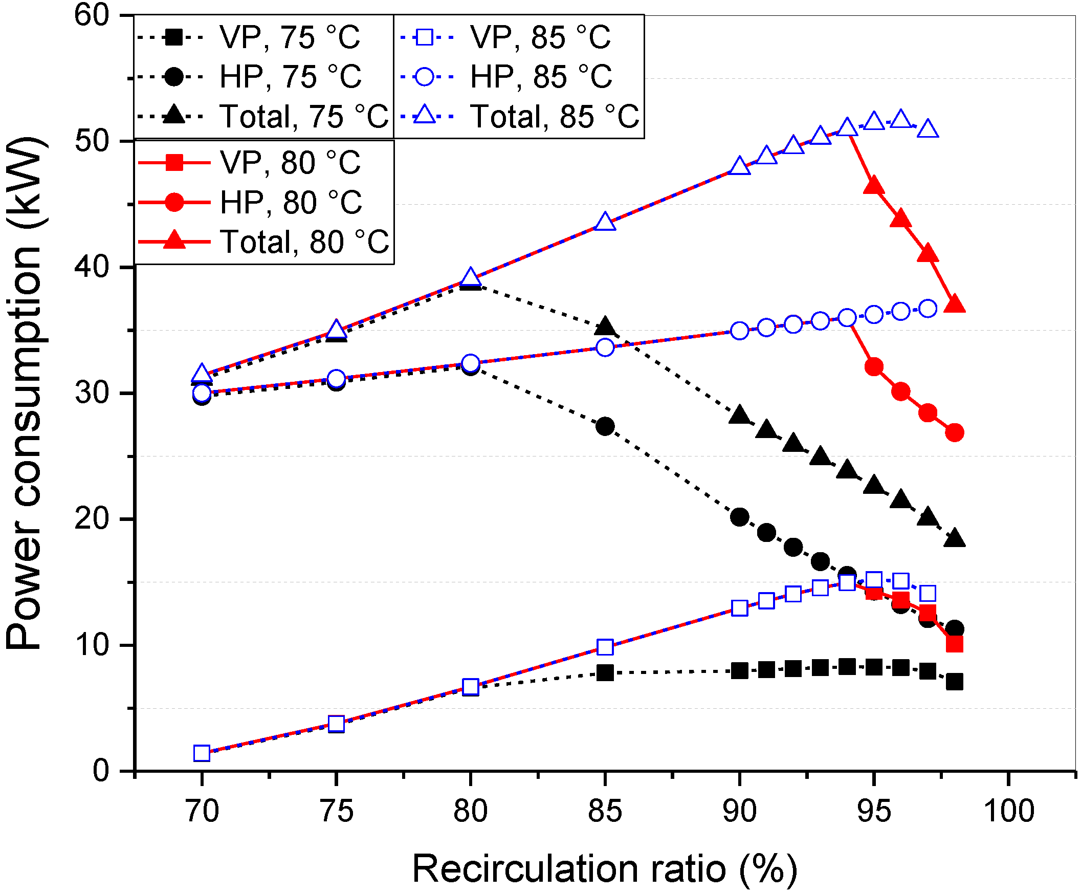
Figure 7 illustrates the electric power consumption for the respective water production for each set-point of the heat pump. The figure presents the required power consumption of the vacuum pump (VP) for the vacuum of 0.26 bar, the heat pump (HP) consumption and the total power consumption of the system as the recirculation ratio increases for the set-point of the heat pump at 75, 80 and 85 °C. The lower consumption is identified for the case of 75 °C where the maximum water production is 0.13 m³/h, the lowest compared to the other cases. It is observed that, when the recirculation ratio is up to 80%, both the vacuum pump and the heat pump’s compressor power consumption increase, leading to an increased total power consumption with a maximum of 40 kW. When the recirculation ratio takes values higher than 80%, the vacuum pump power consumption remains almost constant, while the heat pump and total power consumption decrease, since the largest percentage of the recirculating brine is already hot and the heat pump switches off. A similar behavior can be observed for the set-point at 80 °C, presenting higher total power consumption, while the heat pump reaches the set-point at a recirculation ratio of 93%. Finally, when the set-point of the heat pump is 85°C, the vacuum pump, heat pump and the total power consumption show the highest values and the heat pump does not seem to reach the set point. Figure 8 presents the respective coefficient of performance (COP) for the three cases.

The specific energy consumption in terms of total electricity absorbed by the system is presented in Figure 9 for the three set-points of the heat pump, showing the total energy consumed for each cubic meter of produced water. It can be observed that, for the specific vacuum (0.26 bar) provided by the vacuum pump, the set-point of 75 °C presents the lowest specific energy consumption, while the specific energy consumption of 80 and 85 °C present similar values for the recirculation ratio up to 95%.

3.2. Effect of Pressure Difference Derived by Vacuum Pump

In the previous section, the effect of the heat pump set-point temperature on the system performance and water production was examined. However, the pressure difference applied on the fash tank, which is derived from the vacuum pump, also has a significant impact on the system’s performance. Figure 10 provides the water production for two pressure differences at two different heat pump set-points (75 and 80°C), as the recirculation ratio increases. For the case of 75 °C, it can be observed that, when the recirculation ratio is up to 81%, the highest pressure difference (Δp = 0.8, i.e. vacuum at 0.21 bar) presents higher water production, while for the higher recirculation ratio, a lower vacuum leads to slightly higher water production, up to 0.13 m³/h.

For the case of 80 °C, the pressure difference of 0.75 bar (vacuum 0.26 bar) presents much higher water production, up to 0.2 m³/h, than the pressure difference of 0.7 bar (vauum 0.31 bar).

Figure 11 presents the salinity of the outlet brine flowing out of the flash tank. It is observed that, for a recirculation ratio of more than 95%, the salinity increases significantly for all the cases.

Figure 12 presents the power consumption as the recirculation ratio increases to produce the corresponding quantity of water. Figure 12a shows the vacuum pump, the heat pump and the total power consumption for the pressure difference of 0.75 bar (vacuum 0.26 bar) and 0.8 bar (vacuum 0.31 bar) at the heat pump’s set-point at 75 °C. It is observed that the case with Δp = 0.8 bar presents much higher total power consumption, up to 51 kW, as the recirculation ratio increases up to 93%, as the vacuum pump has a larger load and the heat pump operates to reach the set temperature. Figure 12b depicts the same parameters for the pressure difference of 0.75 bar (vacuum 0.26 bar) and 0.7 bar (vacuum 0.31 bar) for the heat pump’s set-point at 80 °C. The behavior for the two scenarios is similar to the case presented in Figure 12a.

Figure 13 depicts the COP of the heat pump as the recirculation ratio increases for the two different set-points of the heat pump and the pressure differences derived from the vacuum pump. For the set-point of 75 °C, two pressure differences are presented, namely Δp = 0.75 bar (vacuum 0.26 bar) and Δp = 0.8 bar (0.21 bar), showing that the COP decreases for every case when the recirculation ratio is lower than 80%, but after this point, the COP increases with the recirculation ratio, up to 4.15 for Δp = 0.8 bar and 3.66 for Δp = 0.75 bar. This can be explained by the heat pump energy consumption presented in Figure 10, which decreases after the recirculation ratio is 80%, since the brine reaches the set-point temperature, and its compressor reduces the power consumption. For the case of the heat pump’s set-point of 80 °C, the COP reduces with the increase in the recirculation ratio, and drops below 3 when the recirculation ratio equals 85% for Δp = 0.7 bar and 93% for Δp = 0.75 bar, while after this point, the COP increases again up to 3.1 and 3.25, respectively.

It is observed that, for the same vacuum (Δp = 0.75 bar), two different set-point scenarios (75 and 80°C) lead to a COP with a very small difference when the recirculation ratio is up to 80%, while for the recirculation ratio higher than 80%, only a small part comes from RO with a low temperature, and the set-point of 75 °C can be more easily reached, leading to reduced power consumption and higher COP.

Finally, the specific energy consumption for all these scenarios is presented in Figure 14. It is observed that the specific energy consumption reduces significantly as the recirculation ratio increases, presenting a minimum of 170 kWh/m³ of produced water for a recirculation ratio of 98%. Moreover, when the pressure difference is higher, at 0.8 bar, the specific energy consumption is significantly lower for low recirculation ratios compared to Δp = 0.75 bar and Δp = 0.7 bar, while this difference reduces when the recirculation ratio increases. Furthermore, for the same vacuum, the heat pump set-point seems to present the same performance for a recirculation ratio lower than 85%, but for higher values, the specific energy consumption is higher in the case of higher set-point temperatures. As the brine inlet temperature increases, the energy that is lost to the sea discharge is highly increased, since at the set-point of 75 °C, the outlet temperature of the flash tank is 4–5 °C higher than the saturation temperature, while at 80 and 85°C, the temperature difference is much higher, and a part of this brine flow is rejected to the sea, leading to increased specific energy consumption.

3.3. Preliminary Economic Evaluation

A preliminary parametric techno-economic analysis is performed to evaluate the viability of the proposed technological solution for the brine treatment. The analysis is based on the estimation of the levelized cost of water ($\mathrm{LCOW}$) [€/m³]. Levelized costs are commonly utilized in investment planning to compare the different proposed technological solutions. For the proposed system, $\mathrm{LCOW}$ represents the average cost that its owner will have to pay for every m³ of produced freshwater throughout its life cycle. $\mathrm{LCOW}$ is calculated by the following formula:

$$\mathrm{LCOW}=\raisebox{1ex}{${\sum }_{i=1}^{N_t}{\displaystyle \frac{I_i+M_i+E_i}{{\left(1+r\right)}^i}}$}\!\left/ \!\raisebox{-1ex}{${\sum }_{i=1}^{N_t}{\displaystyle \frac{Q_i}{{\left(1+r\right)}^i}}$}\right.$$

(7)

where $N_t$ [years] is the anticipated life cycle of the unit, $r$ [%] is the discount rate, whereas $I_i$ [€], $M_i$ [€], $E_i$ [€], and $Q_i$ [m³] represent the investment cost, the O&M cost, the total cost of electricity, and the total freshwater production in year $i$, respectively.

The following assumptions were considered for the analysis:

• The anticipated life cycle $N_t$ of the unit is 20 years.
• The specific electricity consumption is taken equal to 150 kWh/m³, as it is the minimum electricity consumption of the unit.
• The discount rate $r$ is 3%.
• The annual production of freshwater is equal to 920 m³ (corresponding to 8000 operation hours annually), and it remains constant throughout the unit’s life cycle.
• The investment cost $I_1$ in year 1 is estimated to be about 80,000€, and no investments are necessary thereafter.
• The annual cost $M_i$ is considered constant and equal to 1% of $I_1$.
• An annual increase of 2% in the price of electricity is considered.

A parametric analysis was performed with the cost of electricity $e$ [€/kWh] as the varying quantity, because of the great differentiation in its value based on the installation location and the acute fluctuations noticed in the global energy market during the past few years. The values of $\mathrm{LCOW}$ as a function of $e$ are listed in

Table 4. Estimation of LCOW.

Cost of Electricity, e [€/kWh]	LCOW [€/m3]
0.07	11.78
0.10	15.33
0.15	21.26
0.20	27.18

.

The values of $\mathrm{LCOW}$ are in accordance with the values documented in the literature [29], taking into consideration that brine has an adverse impact on the environment due to its high salinity. The economic viability and competitiveness of the unit will be increased by reducing the cost of the necessary electricity input because the brine treatment process is highly energy-consuming. Ideally, this will be accomplished by integrating renewable energy sources into the system, such as PV collectors.

4. Conclusions

The current study presents a novel brine treatment technology, which is based on the evaporation under a vacuum and a high-temperature heat pump providing the appropriate heating for the brine and cooling for the vapor condensation. The main goal of the paper is to present the key parameters affecting the water production and the electrical energy consumption of the system, in order to minimize the environmental impact and operation cost of the unit. To this end, a quasi-state numerical tool was developed with the use of Matlab Simscape, simulating the flash evaporation and the heat pump operation in varying conditions. The effect of two significant parameters on the system performance was investigated, namely the effect of heat pump set-point temperature and the effect of the pressure difference provided by the system’s vacuum pump, varying the recirculation ratio, which defines the brine flowrate that is rejected to the sea and the brine coming from RO. The study showed that, for a constant vacuum pressure difference, the water production increases with the increase in the set-point temperature and the recirculation ratio. On the other hand, the power consumption for higher set-point temperatures increases, leading to the reduced COP of the heat pump and, in turn, to an elevated specific energy consumption up to 300 kWh per m³ of produced freshwater.

The impact of the vacuum pressure difference was investigated, showing that increased pressure difference provided by the vacuum pump leads to increased water production, but reduces the COP. The specific energy consumption remains lower when the temperature of the heat pump is set at lower levels, while for higher set-point temperatures, the recirculation ratio has an important impact on the specific energy consumption. It is shown that, when the recirculation ratio is up to 87%, a higher vacuum leads to lower specific energy consumption, while for higher values of recirculation, a lower vacuum leads to lower specific energy consumption, with a minimum of 150 kWh/m³ of produced freshwater. Finally, a preliminary economic evaluation of the brine treatment system was accomplished, showing a levelized cost of water that can be competitive with other technologies.

References

1. Panagopoulos, A.; Haralambous, K.J. Environmental impacts of desalination and brine treatment—Challenges and mitigation measures. Mar. Pollut. Bull. 2020, 161, 111773. [Google Scholar] [CrossRef]
2. Cipolletta, G.; Lancioni, N.; Akyol, C.; Eusebi, A.L.; Fatone, F. Brine treatment technologies towards minimum/zero liquid discharge and resource recovery: State of the art and techno-economic assessment. J. Environ. Manag. 2021, 300, 113681. [Google Scholar] [CrossRef]
3. Shatilla, Y. Nuclear desalination. In Nuclear Reactor Technology Development and Utilization, 1st ed.; Khan, S.U.D., Nakhabov, A., Candice, J., Eds.; Woodhead Publishing Series in Energy; Elsevier: Sawston, UK, 2020; pp. 247–270. [Google Scholar]
4. Arafat, H. Brine Management in Desalination Plants. In Desalination Sustainability: A Technical, Socioeconomic and Environmental Approach; Arafat, H., Fedor, J., Eds.; Elsevier: London, UK, 2017; pp. 207–236. [Google Scholar]
5. Rahimpour, M.R.; Kazerooni, N.M.; Parhoudeh, M. Water Treatment by Renewable Energy-Driven Membrane Distillation. In Current Trends and Future Developments on (Bio-) Membranes Renewable Energy Integrated with Membrane Operations, 1st ed.; Basile, A., Cassano, A., Figoli, A., Eds.; Elsevier: London, UK, 2019; pp. 179–211. [Google Scholar]
6. Ghalavand, Y.; Hatamipour, M.S.; Rahimi, A. A review on energy consumption of desalination processes. Desalin. Water Treat. 2015, 54, 1526–1541. [Google Scholar] [CrossRef]
7. Mohamed, A.; Soliman, A.M. A novel study of using oil refinery plants waste gases for thermal desalination and electric power generation: Energy, exergy & cost evaluations. Appl. Energy 2017, 195, 435–477. [Google Scholar]
8. Pangarkar, B.L.; Deshmukh, S.K.; Thorat, P.V. Experimental study of multi-effect membrane distillation (MEMD) for treatment of water containing inorganic salts. Water Pract. Technol. 2016, 11, 765–773. [Google Scholar] [CrossRef]
9. Rivero, R.; Garcia, M.; Urquiza, J. Simulation, exergy analysis and application of diabatic distillation to a tertiary amyl methyl ether production unit of a crude oil refinery. Energy 2004, 29, 467–489. [Google Scholar] [CrossRef]
10. Torres, S.; Acien, G.; Garcia-Cuadra, F.; Navia, R. Direct transesterification of microalgae biomass and biodiesel refining with vacuum distillation. Algan Res. 2017, 28, 30–38. [Google Scholar] [CrossRef]
11. Bin, L.; Ling, C.; Tianyin, L.; Muhammad, S. Chapter 5: Distilled water production by a vacuum heat pump. In Desalination and Water Treatment, 1st ed.; Eyvaz, M., Yüksel, E., Eds.; IntechOpen: London, UK, 2018; pp. 77–95. [Google Scholar] [CrossRef] [Green Version]
12. Almtairi, A.; Sharaf Eldean, A.M.; Soliman, M.A.; Mabroul, A.; Fath, H.E.S. A new preliminary system design of using geothermal well brine heater for desalination/nanofiltration process. Clean. Eng. Technol. 2021, 4, 100213. [Google Scholar] [CrossRef]
13. Ogosu, W.; Danwi, B.; Dagde, K.K.; Akpa, G.J.; Goodhead, O.T. Computer Aided Simulation of Multiple Effect Evaporator for Concentration of Caustic Soda Solution. East Afr. Sch. J. Eng. Comput. Sci. 2020, 3, 146–156. [Google Scholar] [CrossRef]
14. Nafey, S.A.; Abdelaal, M.; Elden, M.A.; El-Maghraby, M.R. Design and Performance Calculation using MATLAB for Multiple Effect Evaporator Desalination Process with Different Configurations. Int. J. Eng. Res. Technol. 2020, 13, 3029–3042. [Google Scholar] [CrossRef]
15. Gao, H.; Jiang, A.; Huang, Q.; Xia, Y.; Gao, F.; Wang, J. Mode-Based Analysis and Optimal Operation of MSF Desalination System. Processes 2020, 8, 794. [Google Scholar] [CrossRef]
16. Said, A.S.; Emtir, M.; Mujtaba, M.I. Flexible Design and Operation of Multi-Stage Flash (MSF) Desalination Process Subject to Variable Fouling and Variable Freshwater Demand. Processes 2013, 1, 279–295. [Google Scholar] [CrossRef]
17. Hassanean, H.M.M.; Nafey, S.A.; El-Maghraby, M.R.; Ayyad, M.F. Simulation of Multi-Stage Flash with Brine Circulating Desalination Plan. JPM Eng. 2019, 21, 34–42. [Google Scholar]
18. Miyatake, O.; Koito, Y.; Tagawa, K.; Maruta, Y. Transient characteristics and performance of a novel desalination system based on heat storage and spray flashing. Desalination 2001, 137, 157–166. [Google Scholar] [CrossRef]
19. Vakilabadi, A.M.; Bidi, M.; Najafi, F.A.; Ahmadi, H.M. Energy, Exergy analysis and performance evaluation of a vacuum evaporator for solar thermal power plant Zero Liquid Discharge Systems. J. Therm. Anal. Calorim. 2020, 139, 1275–1290. [Google Scholar] [CrossRef]
20. Panagopoulos, A. Process simulation and techno-economic assessment of a zero liquid discharge/multi-effect desalination/thermal vapor compression (ZLD/MED/TVC) system. Int. J. Energy Res. 2020, 44, 473–495. [Google Scholar] [CrossRef]
21. ROSA Software. Available online: https://www.wateronline.com/doc/rosa-7-0-0001 (accessed on 30 December 2021).
22. Pinhasi, G.A.; Ullmann, A.; Dayan, A. Modeling of flashing two-phase flow. Rev. Chem. Eng. 2005, 21, 133–264. [Google Scholar] [CrossRef]
23. Liao, Y.; Lucas, D. Computational modelling of flash boiling flows: A literature survey. Int. J. Heat Mass Transf. 2017, 111, 246–265. [Google Scholar] [CrossRef]
24. Mathworks Software. Available online: https://www.mathworks.com/help/matlab/ref/rand.html (accessed on 12 March 2022).
25. Nayar, K.G.; Sharqawy, M.H.; Banchik, L.D.; Lienhard, J.H. Thermophysical properties of seawater: A review and new correlations that include pressure dependence. Desalination 2016, 390, 1–24. [Google Scholar] [CrossRef] [Green Version]
26. Sharqawy, M.H.; Lienhard, J.H.; Zubair, S.M. Thermophysical properties of seawater: A review of existing correlations and data. Desalin. Water Treat. 2010, 16, 354–380. [Google Scholar] [CrossRef]
27. Bell, H.I.; Wronski, J.; Quolin, S.; Lemort, V. Pure and Pseudo-pure Fluid Thermophysical Property Evaluation and the Open-Source Thermophysical Property Library CoolProp. Ind. Eng. Chem. Res. 2014, 53, 2498–2508. [Google Scholar] [CrossRef] [Green Version]
28. Available online: http://www.hanbell.com.cn/En/Skippower/downloadFile/id/70/modelid/57.html (accessed on 12 March 2022).
29. Panagopoulos, A. Techno economic evaluation of a solar multi-effect distillation/thermal vapor compression hybrid system for brine treatment and salt recovery. Chem. Eng. Process. Process Intensif. 2020, 152, 107934. [Google Scholar] [CrossRef]
Figure 1. Desalination unit for brine treatment.
Applsci 12 04542 g001
Figure 2. Phase diagrams for flash evaporation.
Applsci 12 04542 g002
Figure 3. Flowchart of the numerical process.
Applsci 12 04542 g003
Figure 4. Validation of the current model compared with commercial software for the heat capacity and COP estimation at the evaporation temperature of 32 °C.
Applsci 12 04542 g004
Figure 5. Water production (a) and percentage of water recovery of the flash evaporation (b) as recirculation ratio increases, for three different set-points of the heat pump.
Applsci 12 04542 g005
Figure 6. Salinity of the output liquid brine as recirculation increases for varying set-point temperature of the heat pump.
Applsci 12 04542 g006
Figure 7. Vacuum pump (VP), heat pump (HP) and total power consumption as recirculation ratio increases for the set-points of 75, 80 and 85 °C.
Applsci 12 04542 g007
Figure 8. Coefficient of performance (COP) variation with recirculation ratio for the set-points of the heat pump at 75, 80 and 85 °C.
Applsci 12 04542 g008
Figure 9. Specific energy consumption as the recirculation ratio increases for the set-points of 75, 80, 85 °C.
Applsci 12 04542 g009
Figure 10. Water production as the recirculation ratio increases for two set-points at pressure differences, Δp = 0.7, 0.75 and 0.8 bar.
Applsci 12 04542 g010
Figure 11. Salinity of the liquid outlet brine as the recirculation ratio increases, for two set-points at Δp = 0.7, 0.75 and 0.8 bar.
Applsci 12 04542 g011
Figure 12. Power consumption of the vacuum pump, heat pump and the whole system for Δp = 0.75 and 0.8 bar at 75 °C (a) and for Δp = 0.7 and 0.75 bar at 80 °C (b).
Applsci 12 04542 g012
Figure 13. Coefficient of performance (COP) as recirculation ratio increases for Δp = 0.7, 0.75 for the set point at 80 °C and Δp = 0.75, 0.8 bar for the set-point at 80 °C.
Applsci 12 04542 g013
Figure 14. Specific energy consumption as the recirculation ratio increases for Δp = 0.7, 0.75 and 0.8 bar.
Applsci 12 04542 g014