Abstract
Analytic models, complex simulations, and simple models are being used to predict the production performance of hydraulically fractured shale. Analytical models such as decline curve analysis and rate transient analysis are used for a quick evaluation of reservoir performance. However, they have considerable limitations. For instance, decline curve analysis cannot honor the physical phenomena in shale wells that are related to hydraulic fracture, reservoir characteristics, and fluid flow. On the other hand, even though explicit hydraulic fracture modeling is the most comprehensive approach when compared with other traditional techniques, it cannot guarantee to model enough hydraulic fracture effects. Hence, calibration of the model, which commonly is referred to in the oil and gas industry as history matching, becomes a must. However, history matching of an explicit hydraulic fracture model with limited information is time-consuming and cumbersome. Especially history matching of a full field shale gas/oil model with many wells is a daunting task. In this study, we propose a workflow to integrate numerical reservoir simulation and well test analysis. In the workflow, information such as fracture half-length and enhanced effective permeability are obtained from pressure transient analysis and are used to calibrate grid properties in the vicinity of the plane covered by the fracture length and width. Finally, the simulation model is calibrated using pressure and flow rate data, and it is used for the long-term performance prediction of a hydraulic fractured well. The workflow was evaluated by using a synthetic reservoir model whose permeability mimicked that of a shale formation. As a result, the workflow thus enabled the use of coarse grid blocks, which, in turn, reduced the simulation time to just 1.5% of the simulation runtime consumed by a reference fine grid model.
1. Introduction
The extraction of hydrocarbons from a tight formation has attracted considerable attention in recent years. Tight formations are characterized by having low porosity and low permeability. The production of crude oil trapped in such low porosity and low permeability formations require stimulation by hydraulic fracturing [1,2]. Hydraulic fracturing creates fracture networks that are vital for efficient production from such formations. To predict the long- and short-term production performances of the stimulated well, an accurate model of the induced fracture networks is crucial. However, owing to difficulties arising from explicitly modeled fracture networks and transient flow at the stimulated reservoir volume, forecasting the production is complex [3,4].
Multiple studies have proposed empirical and analytical models and workflows that range from simple to more complex ones to predict production from a tight formation such as a shale formation [3,5,6,7,8,9,10]. Well test analysis methods and numerical reservoir simulation are two of the well-established techniques employed to predict production. Despite the successful application of well test analysis techniques to the model drainage area of a hydraulic fractured well [11], analytical models developed for well test analysis may not provide a reliable long-term prediction. This is due to the underlining assumptions used to find an analytical solution of the celebrated diffusivity equation [12]. On the other hand, numerical reservoir simulation, which is based on the first principle models, is capable of long-term prediction [13]. However, the difficulty in modeling fracture networks and the high cost of computation calls for a concerted and demanding effort.
The cornerstone of a numerical reservoir model is a geological model which comprises the physical appearance and static properties of the actual reservoir. Hence, to build the geological model (geocellular model), data obtained from seismic, well logs, routine and special core analysis are applied in multimillion grid blocks that represent the heterogeneity and anisotropy of the structure. In addition, discrete fracture network models are included in the generated grid block system via statistical means. These fractures are clustered, and for each cluster, fracture half-length, fracture height, fracture width, and fracture conductivity are estimated.
Despite having an irregular shape, the induced fractures and fracture networks are represented by a well-rounded geometry, which reduces the accuracy of the model [14]. Moreover, the integration of fracture characteristics in the geocellular model is a rather meticulous task that requires the modification of the starting geological model. Often, local grid refinements are utilized to account for the hydraulic fracture characteristics [15,16,17]. The numerical computation of fluid flow in fine-tuned grid blocks tends to consume a significant amount of computational time.
Explicit hydraulic fracture (EHF) modeling [18], microseismic mapping [15], and stimulated reservoir volume (SRV) [19,20] methods are commonly used to incorporate the impact of fracture and fracture networks. In contrast to other traditional practices such as decline curve analysis and rate transient analysis, a numerical model integrated with the EHF model is most comprehensive and robust [21]. It is descriptive of the impact of hydraulic fracturing during numerical simulation studies [22]. However, the limitation in EHF modeling has led to the development of the SRV [18,20]. The SRV modeling technique lends itself to a simple yet efficient technique for handling the effect of complex and multicluster hydraulic fractures in numerical reservoir modeling and simulation. In the SRV method, a 3D volume is assumed around the hydraulic fractured well [20]. This volume is then assigned with enhanced permeability to account for the impact of the hydraulic fractures. The performance of the reservoir model with modified permeability is then matched with historical data to calibrate the permeability and supposed stimulated reservoir volume. However, it is essential to recognize that the SRV is only the reservoir volume affected by the stimulation; hence, it does not honor the details of the fracture structure and spacing.
Rincones 2014, compared the performance of the SRV method with Arp’s analytical decline curve analysis [23]. It was found that when the hyperbolic decline curve model is systematically used in segments according to flow regimes (by appropriate choice of decline exponent constant), decline curve analysis provides the same result as the SRV method. However, the decline curve analysis requires less effort and time compared to the SRV method. Hence, the SRV method may not be a good option to be used in reservoir simulation. Moreover, the misinterpretation of the stimulated reservoir volume and its aspect ratio, defined by the ratio of height to width and to length, may result in a significant discrepancy of simulation output and the actual performance. In general, capturing important reservoir properties and fully integrating fracture properties in reservoir modeling and simulation by using EHF and SRV is painstaking.
Liu 2016, showed that well test analysis using data acquired during production could provide more detail and reliable information than SRV or EHF methods [24]. The stimulated reservoir volume method should be used only if a single method such as micro-seismic monitoring or pump-off drawdown test is available. Important fracture properties such as reservoir permeability, fracture conductivity, and fracture half-length can be better estimated by well-test analysis. Nevertheless, the analytical model from well testing interpretation alone may not adequately provide long-term prediction because of the underlining assumptions made during the development of the analytical solution to the diffusivity equation upon which well test analysis is based.
On the other hand, reservoir simulation has been successfully employed for long-term prediction, in spite of difficulties to describe hydraulic fracture well behavior [9,25] and high computational time [26]. One of the difficulties in using numerical simulation is the representation of hydraulic fracturing effects [13,27]. In EHF modeling, extremely fine grid blocks are set up near the fractured well, and the fracture properties are distributed based on fracking job characteristics, such as fluid injection rate and proppant volume [28].
On a similar note, well test analysis is efficient in providing critical information such as fracture half-length, effective permeability, and conductivity of a hydraulic fracture well [29,30]. One of the ways to present hydraulic fractured well behavior via well test analysis is by employing high negative skin. While half or quarter slopes in the log–log plot are not captured during well test analysis, negative skin and fracture half-length can be estimated using large-scale grid sizes. This is because, in hydraulically fractured wells, the effective wellbore radius is big.
In this study, a method that combines well test analysis and reservoir simulation is proposed for the efficient and long-term production forecasting of a hydraulically fractured well. The method optimizes gridding of a numerical reservoir simulator by incorporating interpretations obtained from well test analysis. In this study, the grid size is set for the main stress direction with fracture half-length and optimized for the minor stress direction based on simulation results. This allows to effectively utilize the capability of the numerical model with reduced computational time.
2. Methodology
A workflow is presented for the long-term prediction of flowrate and bottomhole flowing pressure. The workflow integrates reservoir simulation and well test analysis for better performance prediction of a hydraulically fractured tight formation. The following five steps discuss the workflow.
- Step 1:
- Estimate fracture half-length and permeability through well testing analysis. In cases where the half slope or quarter slope is not captured in a log–log plot, it can be estimated using negative skin.
- Step 2:
- Construct a grid in the direction of the main stress. A fracture is growing in the opposite direction to the main stress, which is the perpendicular direction of the minimum stress direction. Hence, the common grid size follows the main stress direction. Meanwhile, fine gridding is required in direction perpendicular to the main stress direction. In practice, the longer side could be the general half-length size obtained in step 1. The short side could be around 40 ft or less.
- Step 3:
- To reduce the simulation time, apply dual porosity for the fractured cells only.
- Step 4:
- Match the simulation model to pressure behavior obtained during well testing: For infinite conductivity fracture model, the matching parameter of the simulation model is fracture porosity. On the other hand, for finite conductivity fracture model, the matching parameters are fracture permeability and fracture porosity of the simulation model.
- Step 5:
- Predict performance using the well test matched simulation model.
In order to demonstrate the proposed approach, a synthetic reservoir model with fine grid blocks and an aerial grid size of 5 × 5 ft is constructed using commercial numerical reservoir modeling and simulation software. Some of the important information used to construct the model is generated based on information from several wells found in Northern India. The data used to construct the reference sector model are presented in Table 1. This case is selected to represent a real case model of shale gas formation with a hydraulic fracture.

Table 1.
Reservoir rock and fluid properties of a reference sector model and coarse grid models.
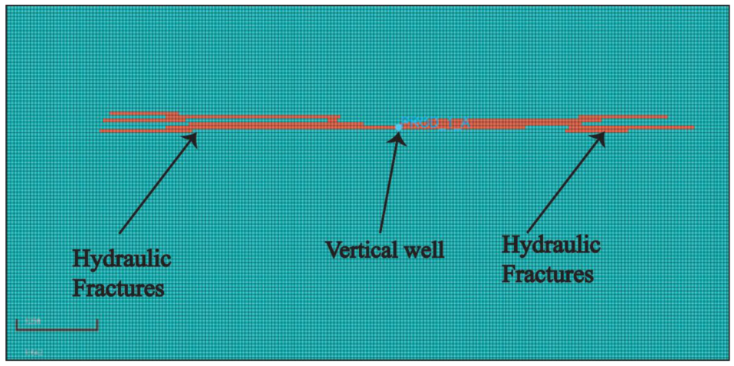
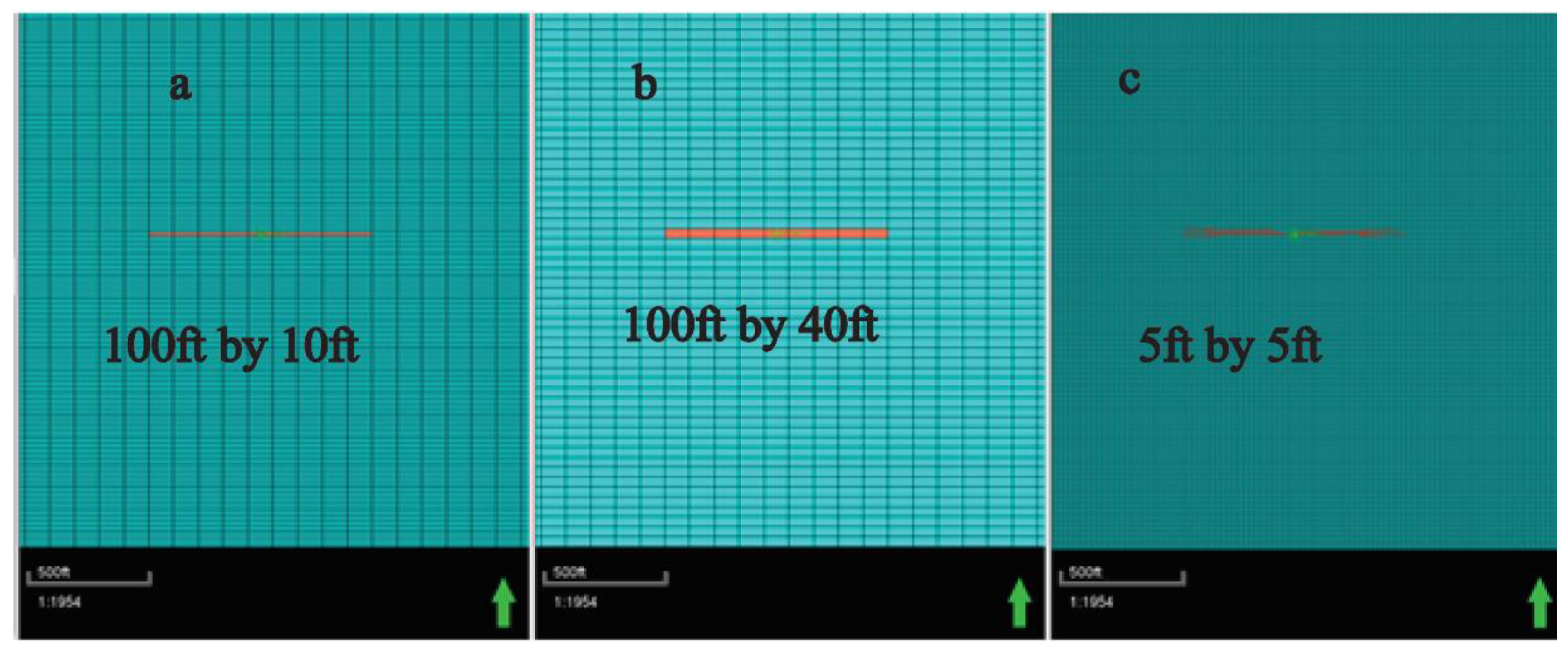
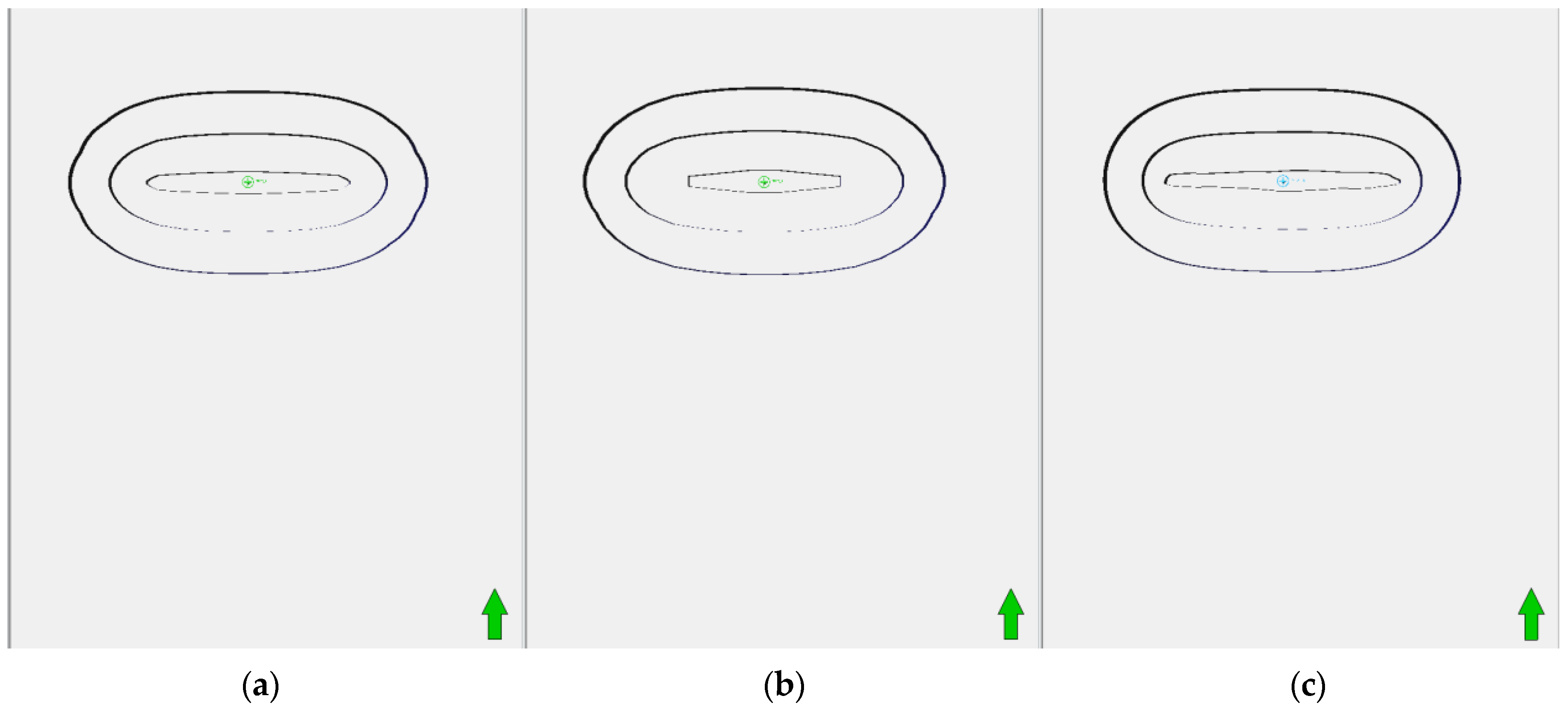
Figure 1 displays the fine grid reservoir model and a vertical well with a hydraulic fracture. Using the same property, two other coarse grid reservoir models, namely coarse grid model 1 and coarse grid model 2, with an aerial dimension of 100 × 10 ft and 100 × 40 ft, respectively, are constructed as shown in Figure 2. The respective data are also presented in Table 1, along with the reference sector model. In order to minimize the simulation run time, only a sector model of the reference synthetic model is used. This is possible by first identifying the drainage area without a boundary effect. A dual-porosity model is used for the fractured area only. In the simulation model, the sigma factor controls the flow between the matrix and the fracture. In the fine grid, the single porosity can be applied to draw a fracture directly; however, in a coarse grid, it is better to use dual porosity in the fracture.
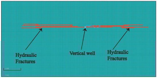
Figure 1.
Synthetic hydraulic fractured well and reservoir.
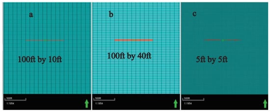
Figure 2.
Coarse and coarser gridding for production performance comparison, (a) Coarse model 1 (b) Coarse model 2, (c) Reference sector model.
3. Result and Discussion
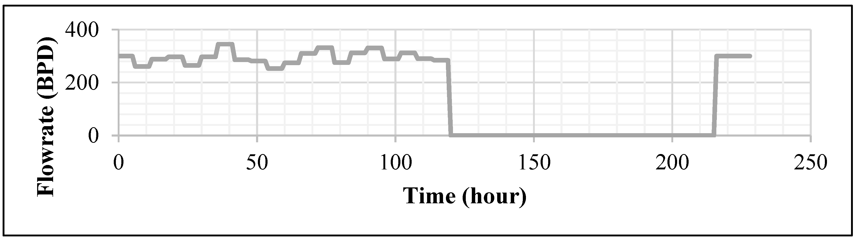
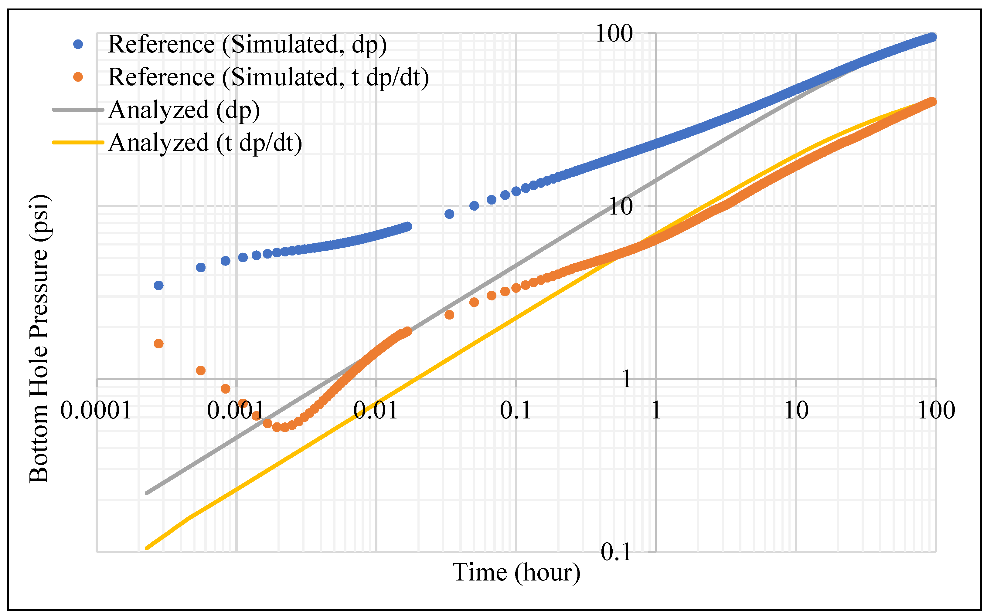
Figure 3 displays the simulated result of a pressure build-up test of the reference model. As presented in the previous section, this case is selected as a reference to represent a real reservoir. Well tests in exploration wells and new wells are often made in a sequence where a drawdown test precedes a build-up test. The build-up test is analytically interpreted by using well-established pressure transient analysis techniques found in many textbooks and the literature. The interpretation can be drawn using methods such as Horner analysis and Miller–Dyes–Hutchinson (MDH) analysis [22]. The detailed description of the equations for pressure transient analysis can be referred to from any well test analysis textbooks. The Horner analysis assumes infinite acting flow at shut-in, which is a short production period. The MDH analysis is based on the opposite assumption that the stable production period before shut-in is very long, and thus pressure changes that originate from the production can be ignored compared to the pressure changes due to a shut-in. The log–log plot analysis is also presented in Figure 4.
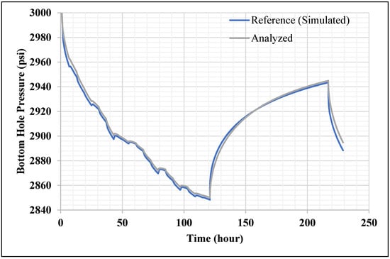

Figure 3.
Analysis of simulation result of the synthetic hydraulic fractured model in Cartesian Plot.
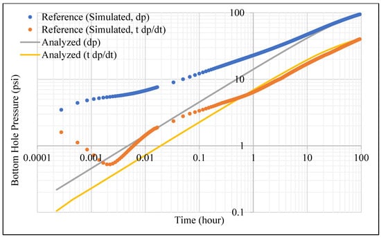
Figure 4.
Analysis of build-up test of the reference model in the log–log plot.
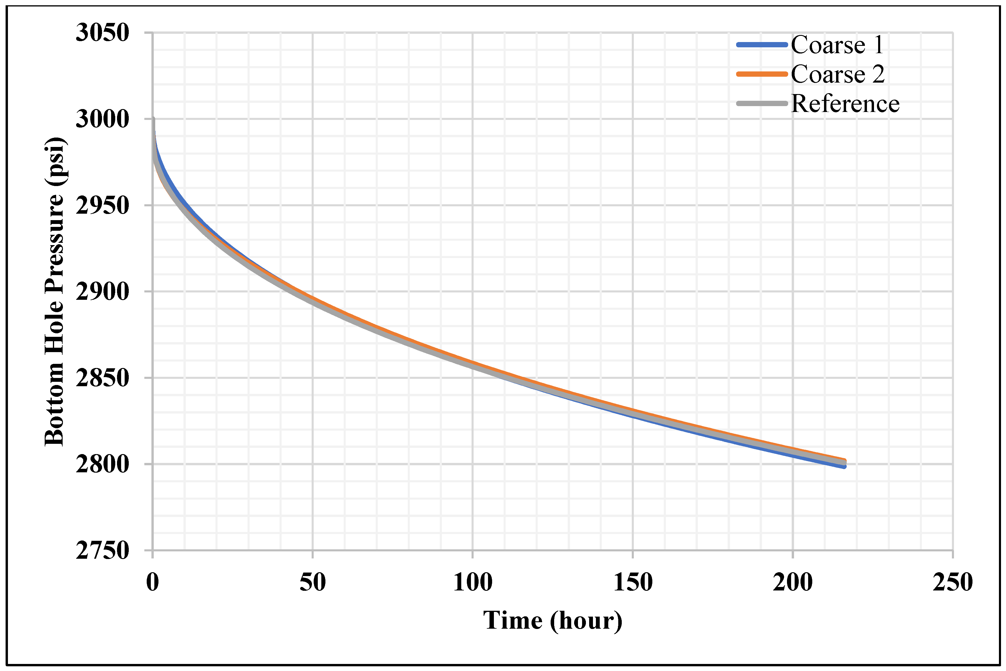
From this analysis, the formation permeability and fracture half-length are estimated to be 0.5 md and 450 ft, respectively. Next, the two coarse grid models presented in Figure 2 are constructed by upscaling the reference model. The grid size along the main stress direction is set to 100 ft, and the size in the perpendicular direction is set to 10 ft and 40 ft for coarse model one and coarse model two, respectively. Dual porosity is set up only for the fractured plane cells. A simulation is run by applying the same constant flowrate tuning to the models. By using the parameters in Table 1, the pressure behaviors are very close to each other.
The pressure results are presented in Figure 5. Here, we simulated an infinite conductivity case (the finite conductivity case can be simulated without difficulty changing fracture permeability). A half-slope straight line on a log–log plot in Figure 4 shows infinite conductivity fracture characteristics [12]. After the linear flow period, the infinite acting radial flow behavior occurs. This model—the infinite conductivity fractured model in well testing interpretation—is based on a fracture plane with zero thickness and total penetration. In the early time (1/2 slope straight line on log–log plot), the pressure drop is based on the area of the fracture plane (thickness × fracture half-length) and formation permeability. Therefore, by taking the inverse of this pressure drop, the formation permeability and fracture half-length could be estimated. As mentioned before, even if the ½ slope is not recognized, the half-length can still be evaluated using negative skin.
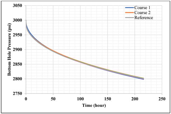
Figure 5.
Bottom hole pressure of the Base Case, Coarse Case, and Reference for a constant flow rate.
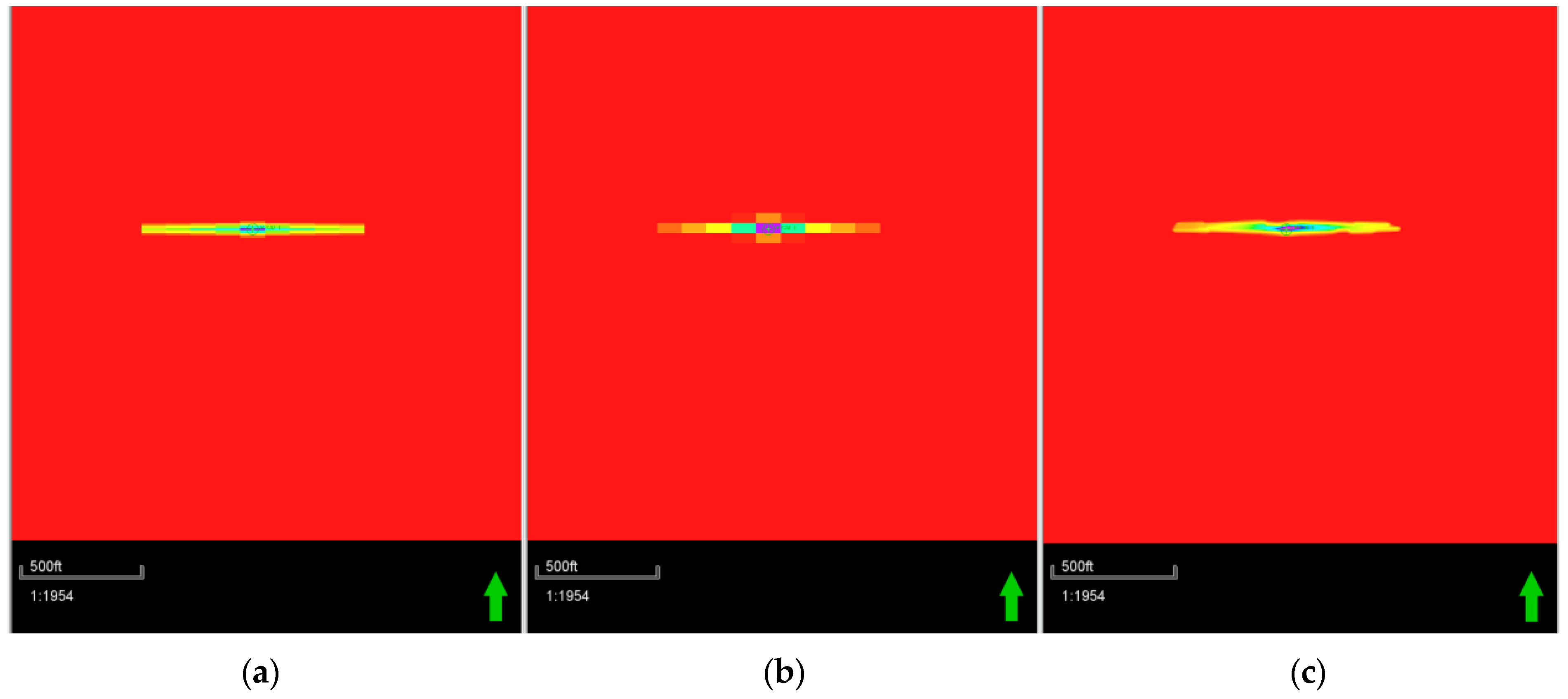
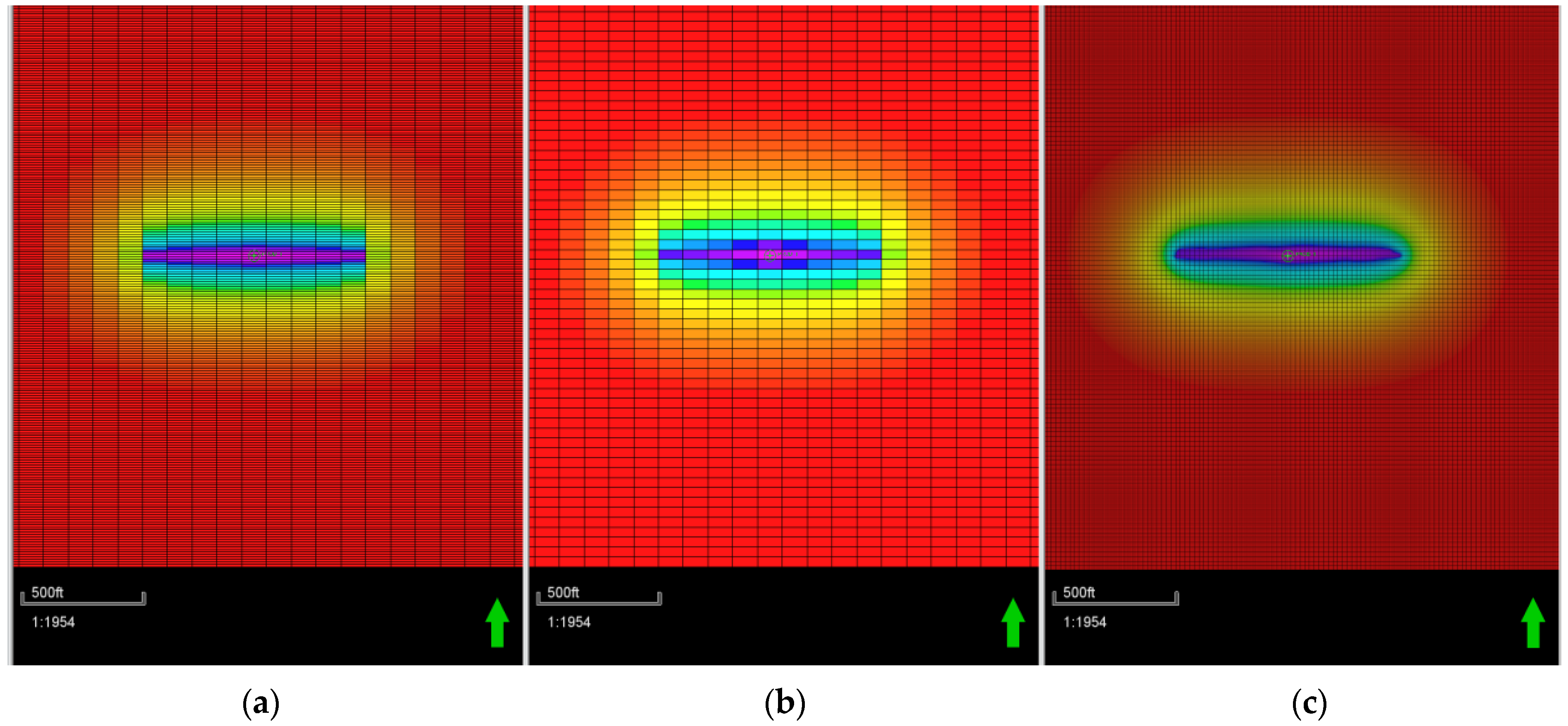
In Figure 6, the early time (9 h) pressure behavior in the reservoir is a little bit different because of the shape of the fracture, even though the bottomhole pressure behavior is very similar, as shown in Figure 5. However, the pressure behavior in the reservoir is very similar at a later time (240 h), as shown in Figure 7 and Figure 8. Those cases will go to a radial flow if there is no boundary effect.
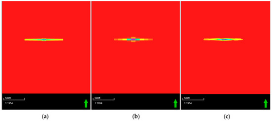
Figure 6.
Pressure map in early time for (a) Base Case, (b) Coarse Case, and (c) Reference.
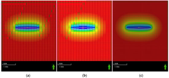
Figure 7.
Pressure map in late time for (a) Base Case, (b) Coarse Case, and (c) Reference.
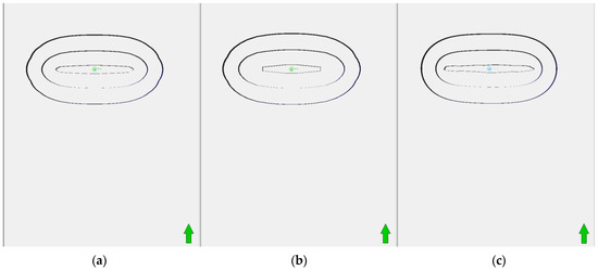
Figure 8.
Pressure contour in early time for (a) Base Case, (b) Coarse Case, and (c) Reference.
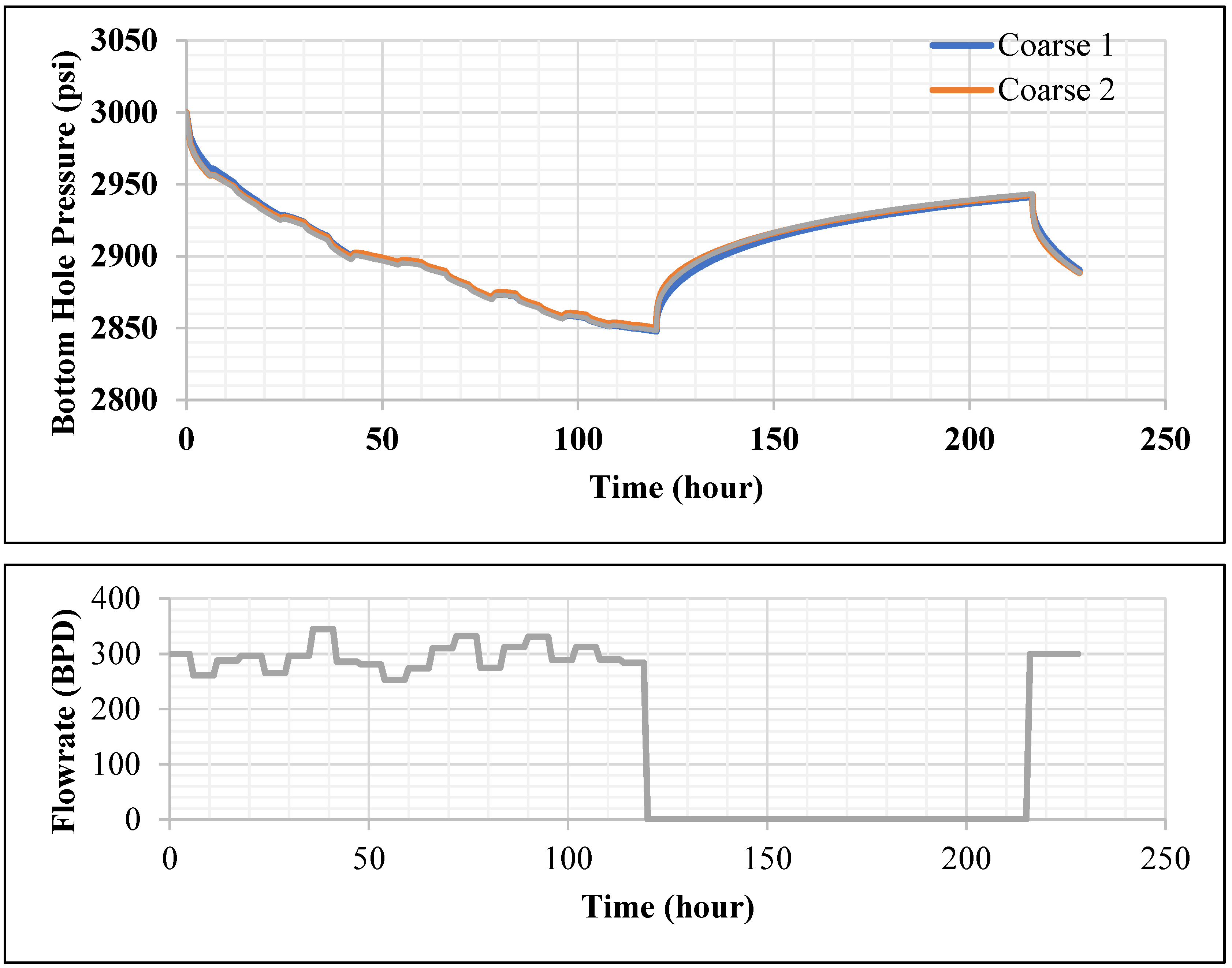
Finally, as shown in Figure 9, coarse models one and two could accurately represent the reference case with a considerably coarsened grid size with only 1.5% of the simulation time. After performing the model setup, the prediction could be performed in a single well as well as in a full field case.
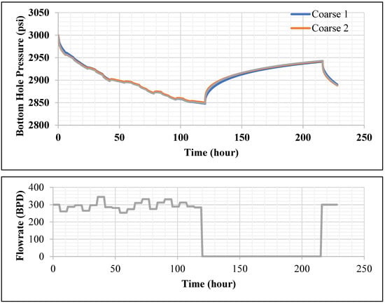
Figure 9.
Bottom hole pressure for Coarse Case and Reference in respectively.
4. Conclusions
This study aimed to show that it is not required to present fracture in the fine grid because fluid/reservoir behavior is very well represented by a single fracture plane. We presented a workflow for modeling the effect of hydraulic fracture on the performance of a synthetic reservoir model. First, a fine grid synthetic reference model which represents a hydraulically fractured reservoir is modeled using data generated based on the information from several wells found in northern India. Two other cases are also developed using the same data but with two different resolutions, i.e., large grid blocks. By calibrating the coarse models with data obtained from the pressure transient analysis, it is shown that their performance closely matches the fine grid performance. The grid shape is a rectangle with long sides that follow the perpendicular direction of the main stress. The size of the grid can be considered normal (not refined) for a long side. Refinement is required for only the short side; however, it can also be optimized. This was especially true at later times when the flow became radial. The proposed method is effective and accurate, and the simulation run times consumed by the coarse grid models were only 1.5% of the reference fine grid models. In addition, by using the unconventional reservoir simulation together with the well test analysis, it is shown that the long-time prediction of the performance of hydraulically fractured reservoir is possible without the requirement of a fine grid model.
Author Contributions
J.H.L., Conceptualization, Funding, Methodology, Software, Writing—original draft preparation; B.M.N., Conceptualization, Methodology, Analysis, Writing—review and editing. All authors have read and agreed to the published version of the manuscript.
Funding
This research received no external funding.
Acknowledgments
The authors would like to express their deepest gratitude for Universiti Teknologi PETRONAS for providing YUTP grants (015LC0-355, 015LC0-412), the required software license and creating the necessary working environment.
Conflicts of Interest
The authors declare no conflict of interest.
References
- Inamdar, A.; Ogundare, T.; Purcell, D.; Malpani, R.; Atwood, K.; Brook, K.; Erwemi, A. Pilot Test Stimulation Approach; The American Oil and Gas Reporter: Haysville, KS, USA, 2011. [Google Scholar]
- Malayalam, A.; Gangopadhyay, A.; Aboubakar, C.; Sebastian, H.; Woodward, D. Reservoir modeling and forecasting shale multi-stage stimulation with multi-disciplinary integration. In Proceedings of the Unconventional Resources Technology Conference, Denver, CO, USA, 12 August 2013. [Google Scholar]
- Suhag, A.; Ranjith, R.; Aminzadeh, F. Comparison of Shale Oil Production Forecasting using Empirical Methods and Artificial Neural Networks. In Proceedings of the SPE Annual Technical Conference and Exhibition, San Antonio, TX, USA, 9 October 2017. [Google Scholar]
- Nejadi, S.; Trivedi, J.J.; Leung, J. History matching and uncertainty quantification of discrete fracture network models in fractured reservoirs. J. Pet. Sci. Eng. 2017, 152, 21–32. [Google Scholar] [CrossRef]
- Makinde, I.; Lee, W.J. Forecasting production of liquid rich shale (LRS) reservoirs using simple models. J. Pet. Sci. Eng. 2017, 157, 461–481. [Google Scholar] [CrossRef]
- Makinde, I.; Lee, W.J. Forecasting Production of Shale Volatile Oil Reservoirs Using Simple Models. In Proceedings of the SPE/IAEE Hydrocarbon Economics and Evaluation Symposium, Houston, TX, USA, 10 May 2016. [Google Scholar]
- Makinde, I.; Lee, W.J. Production Forecasting in Shale Volatile Oil Reservoirs Using Reservoir Simulation, Empirical and Analytical Methods. 2016. In Proceedings of the Unconventional Resources Technology Conference (URTEC), San Antonio, TX, USA, 1 August 2016. [Google Scholar]
- Wang, S.; Chen, S. Evaluation and Prediction of Hydraulic Fractured Well Performance in Montney Formations Using a Data-Driven Approach. In Proceedings of the SPE Western Regional Meeting, Anchorage, AK, USA, 23 May 2016. [Google Scholar]
- Baroni, A.; Delorme, M.; Khvoenkova, N. Forecasting Production in Shale and Tight Reservoirs: A Practical Simulation Method Capturing the Complex Hydraulic Fracturing Physics. In Proceedings of the SPE Middle East Oil & Gas Show and Conference, Manama, BH, USA, 8 March 2015. [Google Scholar]
- Agboada, D.K.; Ahmadi, M. Production decline and numerical simulation model analysis of the eagle ford shale play. In Proceedings of the SPE Western Regional & AAPG Pacific Section Meeting 2013 Joint Technical Conference, Monterey, CA, USA, 18 April 2013. [Google Scholar]
- Imam, K. Evaluating Hydraulic Fracture Properties Using Well Test Analysis on Multi Fractured Horizontal Wells. In Proceedings of the SPE/PAPG Annual Technical Conference, Islamabad, Pakistan, 26 November 2013. [Google Scholar]
- Gringarten, A.C.; Ramey, H.J., Jr.; Raghavan, R. Unsteady-state pressure distributions created by a well with a single infinite-conductivity vertical fracture. Soc. Pet. Eng. J. 1974, 14, 347–360. [Google Scholar] [CrossRef] [Green Version]
- De Araujo Cavalcante Filho, J.S.; Sepehrnoori, K. Simulation of planar hydraulic fractures with variable conductivity using the embedded discrete fracture model. J. Pet. Sci. Eng. 2017, 153, 212–222. [Google Scholar] [CrossRef]
- Zhao, J.; Chen, X.; Li, Y.; Fu, B. Simulation of simultaneous propagation of multiple hydraulic fractures in horizontal wells. J. Pet. Sci. Eng. 2016, 147, 788–800. [Google Scholar] [CrossRef]
- Novlesky, A.; Kumar, A.; Merkle, S. Shale Gas Modeling Workflow: From Microseismic to Simulation—A Horn River Case Study. In Proceedings of the Canadian Unconventional Resources Conference, Calgary, AB, Canada, 15 November 2011. [Google Scholar]
- Gataullin, T. Modeling of hydraulically fractured wells in full field reservoir simulation model. In Proceedings of the SPE 117421 Presented at the 2008 SPE Russian Oil & Gas Technical Conference & Exhibition, Moscow, Russia, 28–30 October 2008. [Google Scholar]
- Ai, S.; Cheng, L.; Liu, H.; Zhang, J.; Huang, S. Production Forecasting of Multistage Hydraulically Fractured Horizontal Wells in Shale Gas Reservoirs with Radial Flow. J. Ind. Intell. Inf. 2014, 2, 303–307. [Google Scholar] [CrossRef]
- Chaudhary, A.S.; Ehlig-Economides, C.A.; Wattenbarger, R.A. Shale oil production performance from a stimulated reservoir volume. In Proceedings of the SPE Annual Technical Conference and Exhibition, Denver, CO, USA, 30 October 2011. [Google Scholar]
- Rubin, B. Accurate simulation of non Darcy flow in stimulated fractured shale reservoirs. In Proceedings of the SPE Western Regional Meeting, Anaheim, CA, USA, 27 May 2010. [Google Scholar]
- Mayerhofer, M.; Lolon, E.; Warpinski, N. What Is Stimulated Reservoir Volume? In Proceedings of the Paper SPE 119890 Presented at Shale Gas Production Conference, Fort Worth, TX, USA, 16–18 November 2008. [Google Scholar]
- Ciezobka, J. Marcellus Shale Gas Project. RPSEA, Annual Report, 2012. Available online: https://www.energy.gov/sites/prod/files/2013/04/f0/2012_annual_plan.pdf (accessed on 29 December 2021).
- Al-Otaibi, B.Z.; Schechter, D.S.; Wattenbarger, R.A. Production Forecast, Analysis and Simulation of Eagle Ford Shale Oil Wells. In Proceedings of the SPE Middle East Unconventional Resources Conference and Exhibition, Muscat, Oman, 26 January 2015. [Google Scholar]
- Rincones, M. Production Forecasting for Shale Oil: Workflow. In Proceedings of the SPE Asia Pacific Unconventional Resources Conference and Exhibition, Brisbane, Australia, 9 November 2014. [Google Scholar]
- Liu, X. Shale-gas well test analysis and evaluation after hydraulic fracturing by stimulated reservoir volume (SRV). Nat. Gas Ind. B 2016, 3, 577–584. [Google Scholar] [CrossRef]
- Cipolla, C.L. Modeling production and evaluating fracture performance in unconventional gas reservoirs. J. Pet. Technol. 2009, 61, 84–90. [Google Scholar] [CrossRef]
- Kazemi, H.; Merrill, L.S.; Porterfield, K.L.; Zeman, P.R. Numerical simulation of water-oil flow in naturally fractured reservoirs. Soc. Pet. Eng. J. 1976, 16, 317–326. [Google Scholar] [CrossRef]
- Liang, B.; Khan, S.A.; Puspita, S.D. An Integrated Modeling Work Flow with Hydraulic Fracturing, Reservoir Simulation, and Uncertainty Analysis for Unconventional-Reservoir Development. SPE Reserv. Eval. Eng. 2017, 21, 462–475. [Google Scholar] [CrossRef]
- Lee, J.H.; Shuhili, J.A.B.M. A Single Equation to Depict Bottomhole Pressure Behavior for a Uniform Flux Hydraulic Fractured Well. Appl. Sci. 2022, 12, 817. [Google Scholar] [CrossRef]
- Egya, D.O.; Corbett, P.W.; Geiger, S.; Norgard, J.P.; Hegndal-Andersen, S. Calibration of naturally fractured reservoir models using integrated well-test analysis—An illustration with field data from the Barents Sea. Pet. Geosci. 2022, 28. [Google Scholar] [CrossRef]
- Kaya, O.A.; Durgut, I.; Canbolat, S. Numerical Modeling of Waterflooding Experiments in Artificially Fractured and Gel Treated Core Plugs by Embedded Discrete Fracture Model of a Reservoir Simulation Toolbox. In Proceedings of the SPE International Conference and Exhibition on Formation Damage Control. OnePetro, Lafayette, LA, USA, 16 February 2022. [Google Scholar]

Publisher’s Note: MDPI stays neutral with regard to jurisdictional claims in published maps and institutional affiliations. |
© 2022 by the authors. Licensee MDPI, Basel, Switzerland. This article is an open access article distributed under the terms and conditions of the Creative Commons Attribution (CC BY) license (https://creativecommons.org/licenses/by/4.0/).