Abstract
Earthquakes are a major external factor that induce landslides. In order to systematically study the dynamic effects and failure mechanism of anti-dip bedding rock slopes (the slope trend is the same as the joint trend, while the slope dip direction is opposite to the joint dip direction) under seismic action (as well as the spatial effects of the structural planes in the anti-dip bedding rock slopes), three-dimensional (3D) discrete-element numerical calculations were performed to analyze anti-dip bedding rock slopes with different slope angles, joint angles, and joint trends subjected to the action of natural seismic and sinusoidal waves. The results were analyzed to investigate the amplification effect, change in Fourier spectrum, failure mechanism, and permanent displacement of the slope under the applied seismic action. The permanent displacement of the slope was calculated using Newmark’s method and the results obtained were discussed and compared with those obtained from a dynamic analysis performed using the 3D discrete-element method. The results showed that the regularity of the spatial distribution of the amplification effect was less clear than that encountered in the planar problem (unidirectional or bidirectional dynamical loading), and this leads to the effect of having an overall rhythmical nature. The seismic wave decays in the high-frequency part from the bottom up of the slope, while the dominant frequency of the seismic wave decreases. The value of the permanent displacement obtained using Newmark’s method is much smaller than that obtained using the dynamic 3D discrete-element analysis approach. The angle between the joint and slope trends has a significant effect on the amplification effect, failure mode, permanent displacement, and stability of slopes subjected to seismic action.
1. Introduction
Flexure toppling failure is widely found in anti-dip bedding rock slopes. According to Goodman and Bray, the toppling failure modes of anti-dip bedding rock slopes can be divided into three categories: block toppling, flexure toppling, and block–flexure toppling, depending on the nature of the structural planes present [1]. To date, a large number of studies have been conducted on these three failure modes in anti-dip bedding rock slopes subject to static (self-weight) conditions. These include theoretical analyses [2,3,4], tests using models and, for example, centrifuges [5,6,7], and numerical analyses [4,6,7]. Therefore, our understanding of the stability (and mechanism responsible for the failure) of anticlinal rocky slopes under static conditions is relatively mature. However, the dynamic response and stability of anti-dip bedding rock slopes under dynamic effects (e.g., seismic and blasting disturbance) are much more complicated compared to those under static conditions.
The 8.0 Ms Wenchuan earthquake that occurred in 2008 induced more than 60,000 landslide hazards and caused more than 20,000 casualties [8]. The recently-initiated Sichuan–Tibet Railway is a major engineering project that includes 12 potential problem areas along its corridor, wherein the basic seismic intensity can reach up to 0.3 g or higher [9]. Therefore, the need to undergo engineering and construction tasks in areas with high seismic intensities, and also the need to generally prevent disasters occurring due to secondary geological hazards such as landslides, have led to new and more stringent requirements being placed on studies focused on the stability of rock slopes subjected to seismic action.
Compared to bedding rock slopes, anti-dip bedding rock slopes are generally more stable under seismic action. However, once the seismic intensity reaches a certain critical value, insidious processes are set in motion that can lead to disaster and the scale of the instability may become enormous (deep failure). Therefore, it is of great engineering significance to study the failure mechanisms and dynamic responses of anti-dip bedding rock slopes under seismic action.
At present, the stability of anti-dip bedding rock slopes subjected to dynamic action is mainly studied using pseudo-static methods, centrifugal model tests, and numerical calculation. The pseudo-static methods usually simplify the problem by separating the dynamic seismic action into inertia forces acting in two directions: the horizontal direction (with the slope facing outwards) and the vertically upward direction. The limit equilibrium and other methods are then used to make refinements compared to static conditions, thus enabling the stability of the slope under the seismic action to be evaluated. This approach thereby converts the original dynamic problem into a static equilibrium problem. Pseudo-static methods are easy to implement and so they are widely used in engineering practice [10]. However, they cannot be used to study the dynamic response of the slope under dynamic action and so they cannot accurately describe the failure mechanism involved. As a result, researchers usually apply pseudo-static methods in combination with other methods to more comprehensively evaluate the stability of slopes under seismic action [11,12,13].
Yagoda-Biran and Hatzor [11], for example, used a pseudo-static method to analyze the ultimate equilibrium state of a single block in a slope and then deduced the relationship between the failure mode of the rock mass and the slope angle, the width-to-height ratio, and the friction angle. Guo et al. [12] derived an analytical solution for the stability of anti-dip bedding rock slopes subject to dynamic action using limit equilibrium theory that can be readily applied to shaking-table tests. Their method predicts that the slumping or sliding of the blocks from the top of the slope to the foot gradually increases as the input acceleration is increased, while the safety factor gradually decreases. Their results were further shown to be in full agreement with the deformation characteristics and stability conditions encountered in shaking-table tests. Zheng et al. [13] combined a pseudo-static method with a genetic algorithm approach to create a new way of evaluating the dynamic stability of anti-dip bedding rock slopes. They found that dynamic failure surfaces are formed in the anti-dip bedding rock slope that are all step-like in nature and the form of the slope’s failure surface and stability are closely related to the strength of the rock.
Shaking-table tests can realistically simulate the instability of rock slopes subject to dynamic disturbance by, for example, earthquakes. Meanwhile, the dynamic effects and failure processes in slopes can be analyzed by setting up appropriate displacement and acceleration monitoring points in the test models. However, the experimental process is time-consuming, costly, and complicated to operate. Shaking-table tests have been carried out by previous researchers for different types of anti-dip bedding slopes (using appropriate model ratios) based on seismically-unstable slopes that have already undergone failure [14,15,16].
Fan et al. [14] investigated the dynamic responses and failure mechanisms of bedding and anti-dip bedding rock slopes with siltized intercalation using shaking-table tests. Their results suggest that both bedding and anti-dip bedding rock slopes begin to exhibit dynamic response characteristics that are nonlinear when the intensity of the incoming seismic wave exceeds 0.3 g. Chen et al. [15] designed a test model based on Goodman’s mechanical model and used it to investigate the failure modes of blocks under different dynamic conditions. They found that the order in which blocks undergo toppling under the dynamic action directly depends on their slenderness ratio. Ning et al. [16] studied the evolution of the failure process in anti-dip bedding slopes subjected to seismic action using shaking-table tests. In their work, they chose to use an engineering background for their slopes matching the upper part of the Yalong River in China; they also verified their results by carrying out numerical analysis. Their results indicate that the failure process in anti-dip bedding slopes subjected to seismic action can be divided into four stages of evolution: tensile crack development in the stratum, tensile crack formation at the top of the slope, formation of a collapse zone, and instability.
When a slope is subjected to seismic action, the conditions experienced are understandably complex. Under such circumstances, numerical simulations provide an easier way to perform investigations compared to other methods and the results obtained can be more mature and reliable. At present, a variety of numerical computational methods (e.g., finite-element, discrete-element, and finite-difference methods) have been widely applied to analyze the stability of anti-dip bedding rock slopes subjected to seismic action [17,18,19].
Zhang et al. [17] used the Universal Distinct Element Code (UDEC) software package to conduct a dynamic 2D analysis of anti-dip bedding rock slopes subjected to different natural seismic wave. Under different seismic effects, their results suggest a tensile state dominated at the surface of the slope, and a shear state dominated at the toe or in the deep part of topplings. Fan et al. [18] performed a dynamic analysis of anti-dip bedding slopes with siltized intercalation using a finite-difference method and found that the slope first undergoes shear failure in the siltized intercalation zone. Zheng et al. [19] used UDEC to conduct a dynamic 2D discrete-element analysis of reinforced anti-dip bedding rock slope (reinforced using pre-stressed cables) subjected to seismic action and compared the results with those that were not reinforced. It was found that the use of pre-stressed cables is a very effective way of reducing the deformation suffered by anti-dip bedding rock slopes exposed to seismic activity.
In summary, a great deal of research has been conducted on the seismo-dynamic response and stability of anti-dip bedding rock slopes using different methods, and some significant results have been achieved. However, little research has been carried out on the following two aspects: (i) Natural seismic waves occur in the form of U–P, E–W, and N–S three-directional loading: the U–P waves are primary waves (P-waves), and the E–W and N–S waves are east–west and north–south secondary waves (S-waves), respectively. The research conducted so far has been limited to the conditions appropriate to model experiments and 2D numerical simulations. Generally, therefore, only two of the above components are considered. This simplifies the actual three-dimensional (3D) space problem by approximating it as a plane-strain problem. Thus, the current approaches cannot fully and correctly model the real instability state of anti-dip bedding rock slopes in the presence of natural seismic waves. (ii) Current research focuses on ideal anti-dip bedding slopes, i.e., slopes in which the dip direction of the joints is opposite to the dip direction of the slope surface (180° difference) and so the joint trend is exactly the same as the slope trend. However, in reality, there is usually a small angle (5–20°) between the joint and slope trends.
Therefore, in this paper, 3D discrete-element modeling is performed using the software package 3DEC (ver5.20, Itasca, 2019, Minneapolis, MN, USA) in order to analyze the dynamics of anti-dip bedding rock slopes with different joint angles and different slope angles under the action of natural seismic and sinusoidal waves loaded in the E–W, U–P, and N–S directions. Our aim is to reveal the real 3D dynamic responses of anti-dip bedding rock slopes (and the mechanism responsible for their failure), and to obtain the permanent displacements of the slopes, (which we can then compare to those obtained using Newmark’s method).
In addition, we also study the spatial effects of the structural planes to reveal the amplification effects, failure modes, and permanent displacements of anti-dip bedding rock slopes with different angles between their joint and slope trends.
2. Numerical Modeling Using 3D Discrete Elements
2.1. Overview
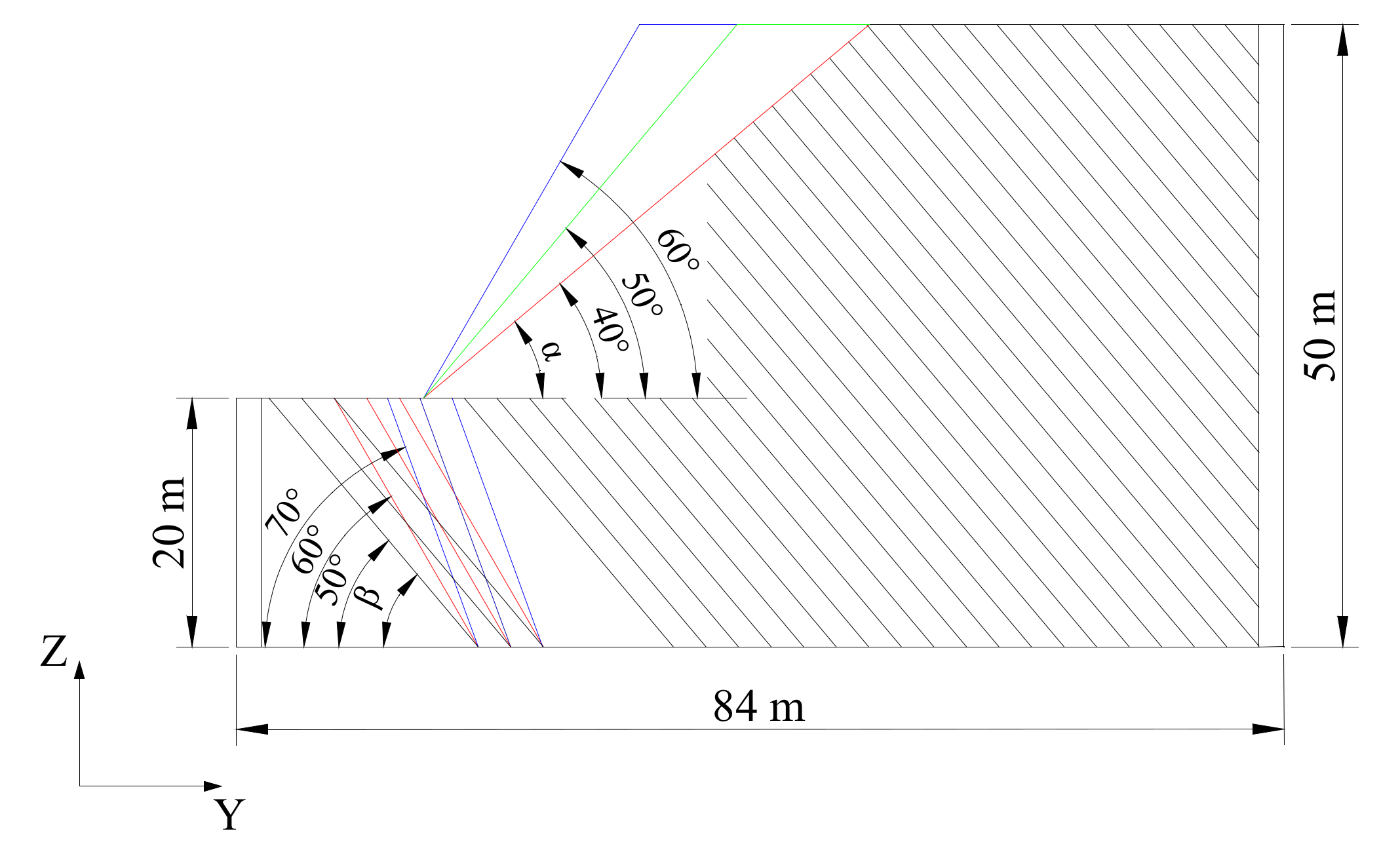
We want to evaluate the effect of varying the slope angle α, joint angle β, and the angle γ between the joint and slope trends on the dynamic response and permanent displacement of anti-dip bedding rock slopes subjected to dynamic action. Therefore, nine 3D discrete-element models (pairwise correspondence, nine combinations, γ = 0°) were first established using slope angles α of 40°, 50°, and 60° and rock angles β of 50°, 60°, and 70° (Figure 1). Eight 3D discrete-element models were subsequently built with γ values corresponding to –20°, –15°, –10°, –5°, 5°, 10°, 15°, and 20°, while the other angles were fixed at α = 40° and β = 70° (Figure 2).
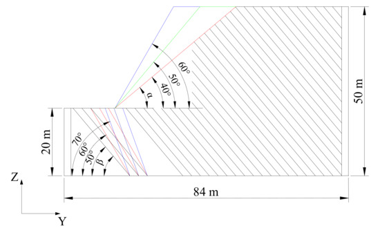
Figure 1.
Side view of the discrete-element model of the slope.
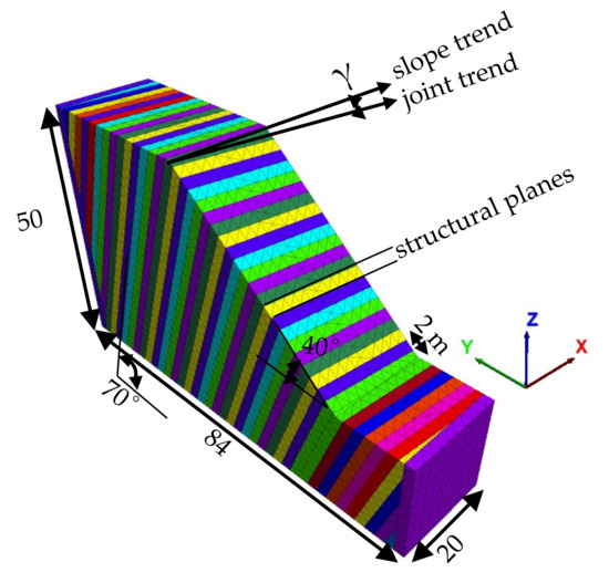
Figure 2.
Three-dimensional view of the slope model.
The sizes of the 3D models correspond to 84 × 20 × 50 m (length × width × height), and the structural planes are equidistantly spaced at 2 m. The slope dip direction is opposite to the joint dip direction geometrically. The Mohr–Coulomb failure model was used for the rock mass and the Coulomb slip failure model was used for the structural planes—the relevant physical and mechanical parameters are presented in Table 1. The normal Kn and tangential Ks stiffnesses of the structural surfaces in the table were calculated using the expressions:
where K is the bulk modulus, G is the shear modulus, E is the Young’s modulus, and ΔZmin is the minimum width in the direction of normal contact of the adjacent units in the discrete-element model [20].

Table 1.
Physical and mechanical parameters used for the rock mass and structural planes.
2.2. Setting the Dynamic Parameters
Unlike the general static case, when numerical analysis is performed under dynamic conditions careful consideration must be given to the relevant dynamic parameters and conditions so that appropriate values can be chosen. Usually, the model must first be run under static (i.e., gravity-only) conditions until static equilibrium is reached. Thereafter, the dynamic analysis can be performed.
The grid size of the model is set to 2 m in order to satisfy the relationship , which is necessary to ensure the accurate propagation of the stress waves within the rock mass [21], where —grid size and —wavelength. Rayleigh damping is also introduced into the dynamic analysis to account for damping phenomena:
where is the mass matrix, is the stiffness matrix, is the critical damping ratio, and is the circular frequency. In this paper, the values = 0.02 and = 5 Hz are adopted.
The bottom of the model was chosen to be a viscous (no-reflection) boundary, that is, separate dampers were set in the normal and tangential directions at the bottom of the model to provide viscous normal and tangential traction, respectively. Free field boundaries were adopted on the four sides of the model to simulate free field motion (Figure 3).
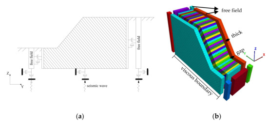
Figure 3.
Schematic diagrams illustrating the dynamic boundary conditions imposed on the 3D discrete-element models showing: (a) a side view of the model, and (b) a 3D spatial view.
As the bottom of the model is set to be a viscous boundary, the dynamic load should be converted from acceleration history to velocity history (by integration) and then to stress history according to:
which are applied to the bottom of the model, where and are the applied normal and shear stresses, respectively, is the rock density, and are the speeds of the P- and S-waves, respectively, and and are the normal and tangential velocities, respectively.
In this paper, two types of dynamic loads were used in the dynamic analysis corresponding to sinusoidal and natural seismic waves. The whole dynamic process lasted 6 s. The expressions for the acceleration history of the sinusoidal waves in the three directions are all in the form: —see Figure 4—the corresponding velocity history is therefore given by ). In this paper, the parameter values adopted are: = 5 Hz for the frequency, because the main energy of the earthquake is concentrated in this frequency band; and = 3.14 m/s2 for the amplitude as these values correspond to a natural Wechuan earthquake in 2008, of intensity Ms = 8.0 [22].
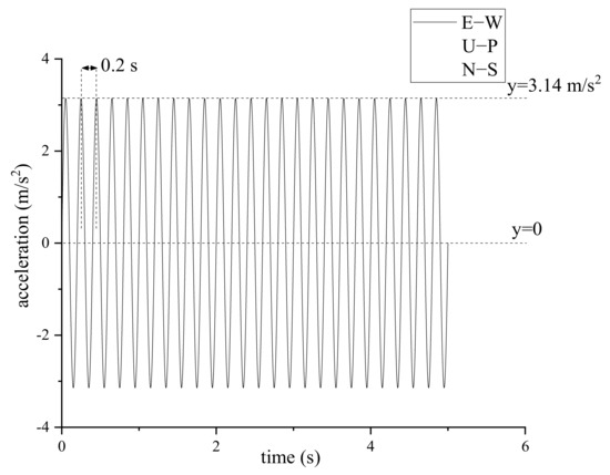
Figure 4.
The input acceleration history of the sinusoidal wave used. The holding time is assumed to be 5 s, the amplitude 3.14 m/s2, and the period (T) 0.2 s.
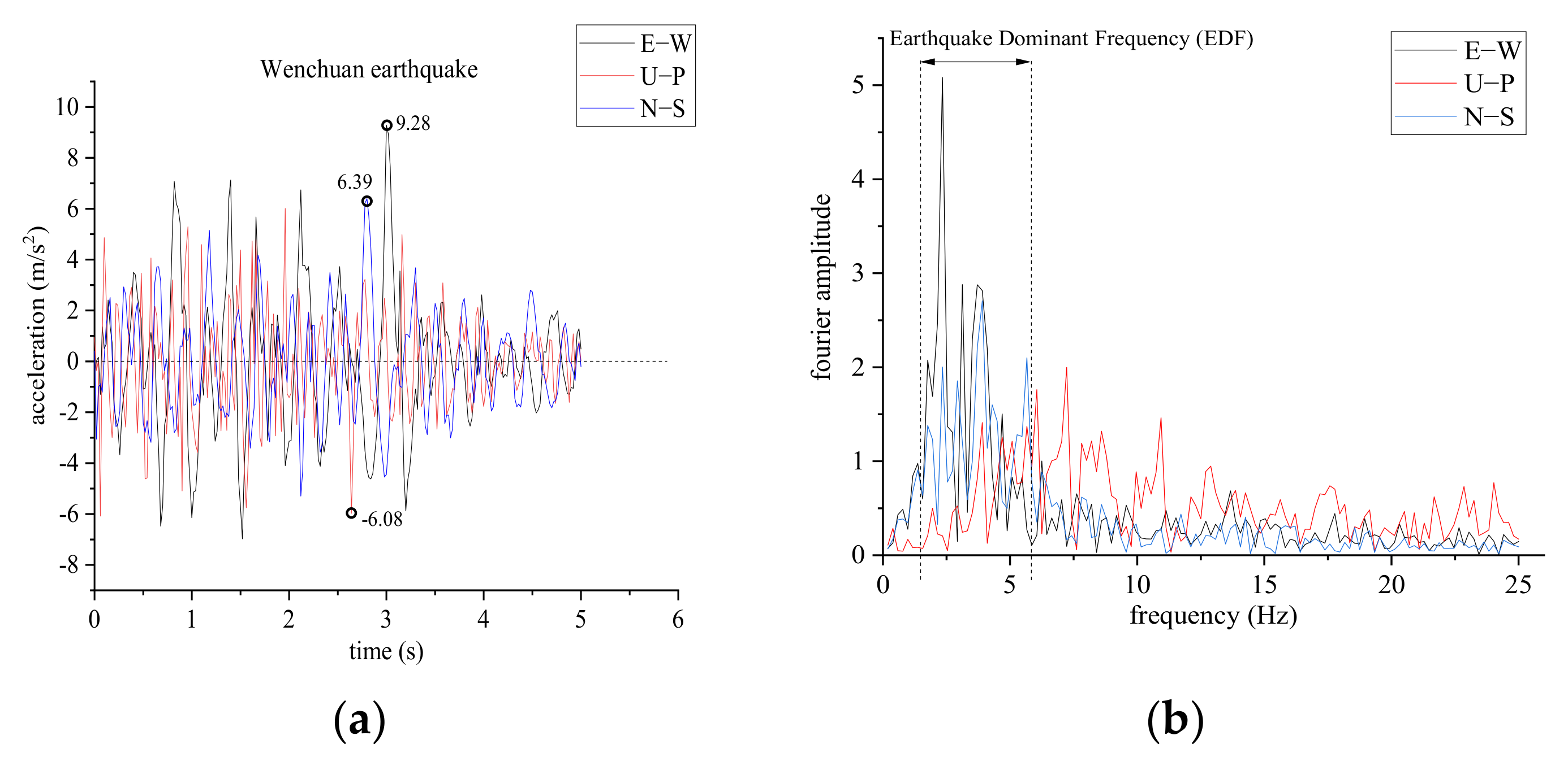
The natural seismic waves used for U–P, E–W, and N–S three-directional loading are taken to have a 5 s acceleration history, which is derived from the Wolong seismic wave of the 2008 Wenchuan earthquake (Ms = 8.0, with an Arias intensity = 5.85 m/s and PGA = 9.28 m/s2)—see Figure 5. The input acceleration history must be baseline corrected to suppress zero drift, that is, it must satisfy , which ensures that the deformation failure of the model is caused only by the dynamic load.
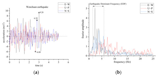
Figure 5.
The nature of the input acceleration used in this work (Wolong waves of the Wenchuan earthquake), showing: (a) the acceleration history with a holding time of 5 s and E–W, U–P, and N–S PGA values of 9.28, 6.39, and −6.08 m/s2, respectively, and (b) the corresponding Fourier spectra and earthquake dominant frequency range (1.5–6 Hz).
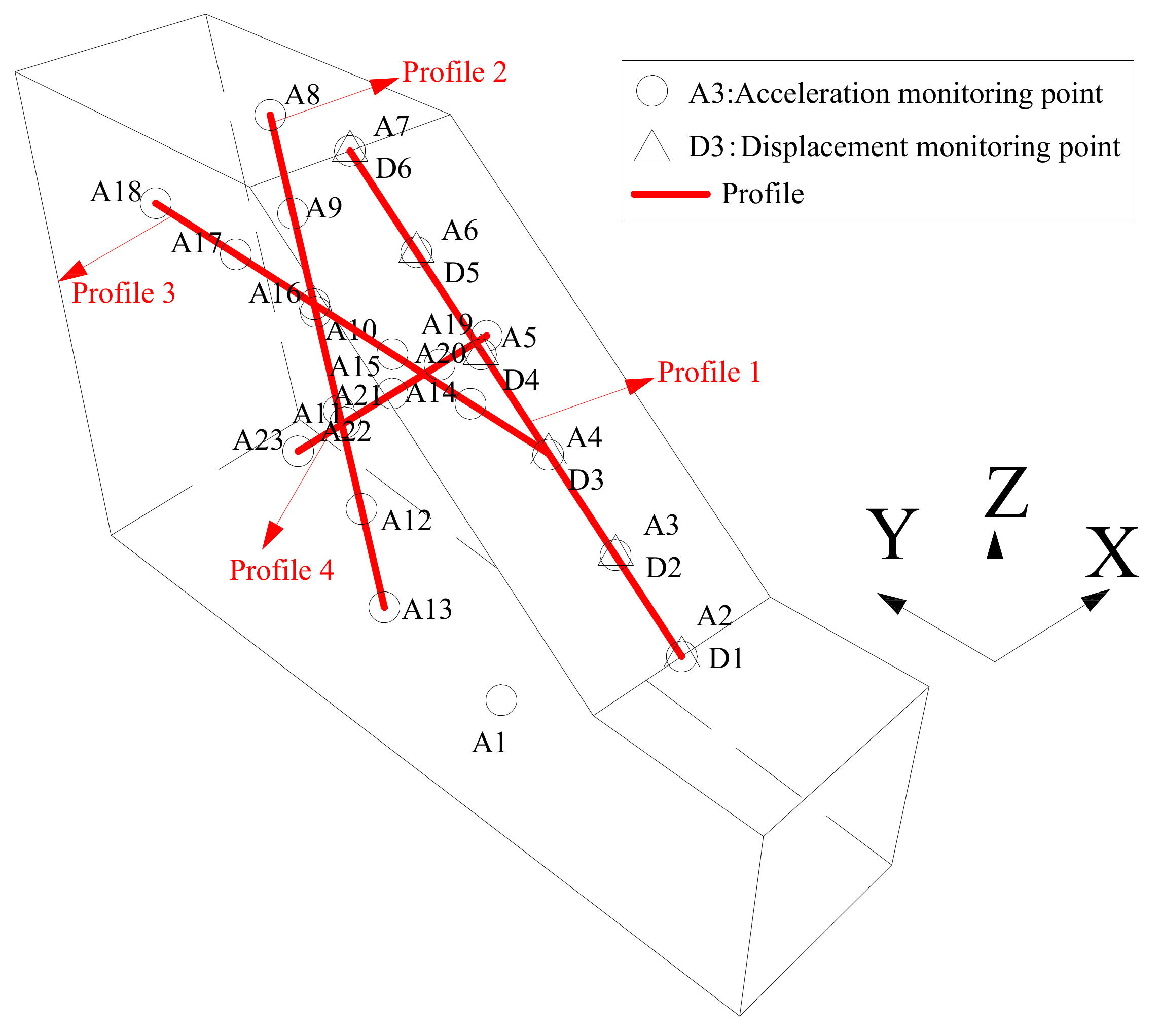
In order to analyze the dynamic amplification effect and variation of the permanent displacement of the slope under dynamic action, 23 XYZ three-directional acceleration calculation points and 6 XYZ three-directional displacement calculation points located on four straight lines were set up inside and on the surface of the slope (Figure 6). These were used to monitor the changes in three-directional acceleration and displacement of the slope model with time during the dynamic loading process.

Figure 6.
Spatial locations of the acceleration (A) and displacement (D) monitoring points and the profiles upon which they are located in the slope model.
Referring to the previous related research methods, and considering the three-dimensional space problem, which is the focus of this paper, the measuring points are distributed equidistantly along the three directions of XYZ. Point A1 is located at the center of the bottom of the model. Points A2–A7 and Points D1–D6 are located on the midline of the slope’s surface (profile 1). Points A8–A13 are located on profile 2 which points in the Z-direction. Points A14–A18 (along with A4) are located on profile 3 which points in the Y-direction. Points A19–A23 are located on profile 4 which points in the X-direction.
3. Dynamic Response of the Slope
3.1. Analysis of the Amplification Effect
The dynamic response of the slope is most intuitively represented by specifying the increase in acceleration experienced by each part of the slope compared to the initial input dynamic acceleration, i.e., the amplification effect. For the sake of simplicity and clarity, the acceleration amplification factor (AAF) calculated using PGA values is usually used to evaluate the amplification effect, i.e., the PGA value measured at a particular point is compared (ratioed) with the PGA value of the initial dynamic input [23,24].
In this paper, the AAFs in the X-, Y-, and Z-directions are denoted by AAFx, AAFy, and AAFz, respectively, and are calculated using the expressions:
where xPGAn, yPGAn, and zPGAn are the PGA values measured in the three directions at a given point in the model and xPGA0, yPGA0, and zPGA0 are the input PGA values in the three directions at the bottom of the model (point A1).
The regularity of the spatial distribution of the dynamic amplification effect inside the model is considered first. Figure 7 shows the AAF results obtained using a slope model with α = 40° and β = 60° when the slope is subjected to dynamic loading in the form of natural seismic waves and sinusoidal waves. Overall, the AAFs produced using sinusoidal waves are generally larger than those produced using natural seismic waves (and their spatial variation pattern is also more obvious). We can compare these results with those obtained in previous research where the amplification effect in anti-dip bedding rock slopes subjected to seismic action was derived using test models and numerical simulations [17,24,25]. According to Figure 7a,b, the slope does not exhibit a single ‘elevation effect’ under the action of three-directional dynamic loading. More specifically, in the plane problem, the AAFs increase monotonically as the elevation increases—here, however, the maximum values appear in the middle and upper parts of the slope (i.e., points A5 and A9). Similarly, it can be found that the ‘surface effect’ that occurs in the plane problem (in which the larger AAF values are encountered closer to the surface of the slope) does not appear under three-directional loading conditions. Instead, according to Figure 7c, the largest AAF values are concentrated at the trailing edge (i.e., points A16–A18) and are further away from the slope surface. We also note that, on the whole, the three-directional accelerations along profiles 1, 2, and 3 do not increase monotonically. Instead, a pattern of increasing (decreasing) values at first followed by decreasing (increasing) values is found.
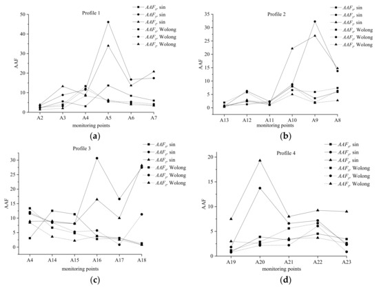
Figure 7.
Variation of the acceleration amplification factors at different acceleration monitoring points due to the action of natural seismic and sinusoidal waves for points along profiles: (a) 1, (b) 2, (c) 3, and (d) 4.
According to elastic wave scattering theory, the seismic S-wave is split when it interacts with a structural plane and is decomposed into a reflected S-wave and refracted P-wave. When a wave propagates from the bottom of the slope to the top it passes through several structural planes and so a complex vibrational wave field is formed within the slope. As a result, a rhythmic pattern of variation is generated in the AAFs. According to Figure 7a,b, we find that AAFz > AAFy in the upper part of the slope and vice versa in the lower part. This coincides with the regularity of the results derived from shaking-table tests conducted by previous workers [26]. This phenomenon can also explain the large amount of horizontal throwing failure that occurred on the slopes during the Wenchuan earthquake. Figure 7d further shows that the high AAF values are concentrated on one side of the slope (point A20), i.e., they are not axisymmetric along the width direction of the slope (X-direction).
Overall, the spatial distribution of the slope amplification effect in the case of three-directional dynamic loading is much less regular than that in the case of the planar problem (one- or two-directional dynamic loading). The AAFs in each direction also have larger increases compared to those in the planar problem. Intuitively, this is also a reflection of the complexity of the propagation and mutual superposition effects of the three-directional seismic waves within the rock mass of the slope.
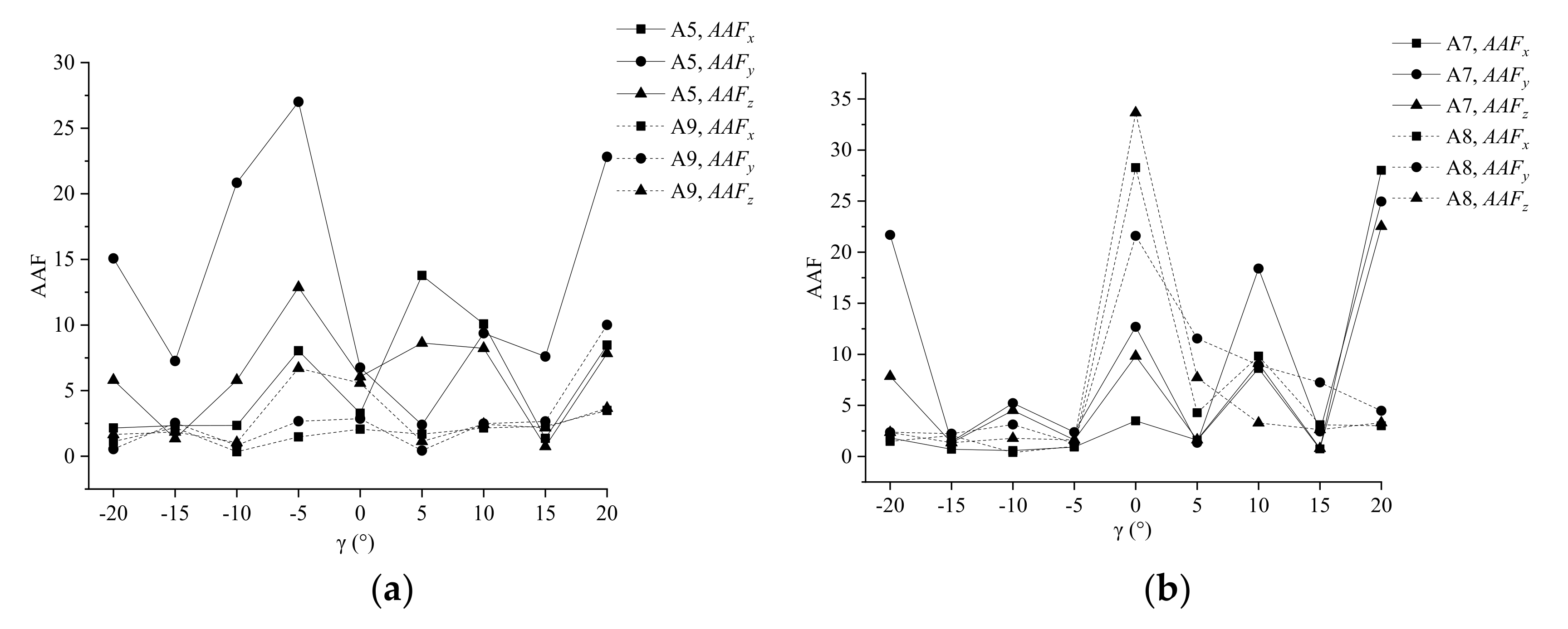
In order to investigate the effect that the regularity of the structural planes has on the slope amplification effect, the variation of the AAFs in the upper part of slopes subjected to the action of sinusoidal waves was studied for different values of γ (angle between the joint and slope trends; the slope and joint angles were fixed at 40° and 70°, respectively). The results are shown in Figure 8. It can be seen that the amplification effect is strong in the upper part of the slope (Figure 8b) when γ is small (−5° to 5°). Then, as γ increases, the AAF values tend to decrease and then increase again when a certain angle is reached (~15°). That is, there is a certain regularity in the AAF values (showing an overall decrease at first and then increasing again). This phenomenon can also be used to visualize the direct relationship between energy dissipation and angle of incidence when a seismic wave is reflected/refracted. It also confirms that the spatial effect of the structural planes is an important factor that cannot be neglected when studying the dynamic response of an anti-dip bedding slope subjected to earthquake activity.
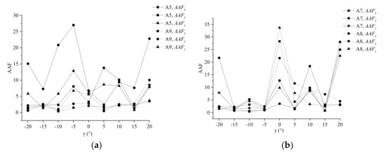
Figure 8.
Variation of the peak acceleration amplification factors at four different points in slopes subjected to the action of sinusoidal waves. The values are plotted as functions of the angle γ and the points chosen are: (a) A5 and A9, and (b) A7 and A8.
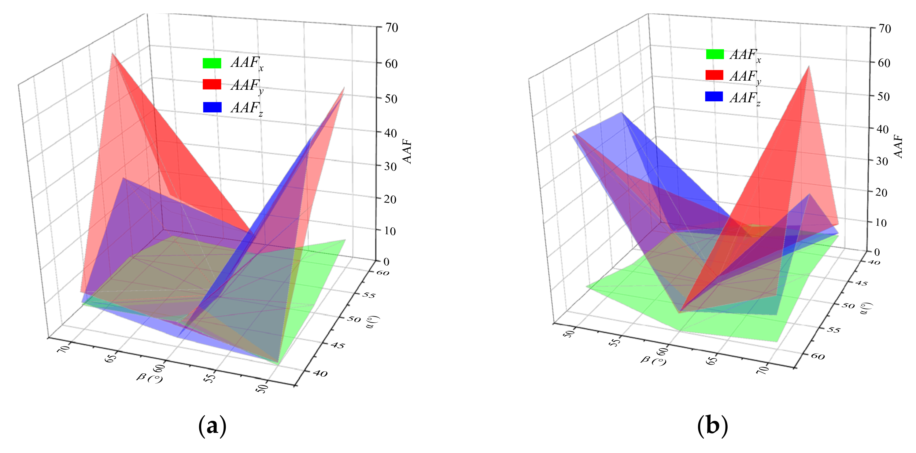
The effect of slope geometry (i.e., slope angle α and joint angle β) on the amplification effect was also investigated. The point A8 at the top of the slope was selected for this purpose. Figure 9 shows surface plots of the AAF results for slopes subjected to sinusoidal and natural seismic waves for different values of α and β. Overall, in both cases, the magnitudes of the components decrease in the order AAFz > AAFy > AAFx. In fact, the AAFx component essentially remains constant and does not vary much as α and β are changed. Thus, the geometry of the slope has a stronger influence on the diffraction and superposition of seismic waves in the YZ-plane (while it has almost no effect in the XY-plane). The trends in AAFy and AAFz are basically the same, i.e., they both increase and then decrease as the slope angle α increases, and decrease and then increase as the joint angle β increases. The largest values of AAFy and AAFz occur when α = 50° and β = 50° and 70°, and the smallest values occur when α = 50° and β = 60°. It is not difficult to find that both the slope angle α and the joint angle β have significant effects on both AAFy and AAFz, because they directly determine the way seismic waves propagate within the rock and the intensity of diffraction, which is intuitively reflected in the magnitude of AAF. In addition, by comparison, it is found that the joint angle β has more influence on AAF compared with the slope angle α, because the rock layers are evenly distributed in the slope, and their quantity is much larger than the slope surface of the slope, so it has more influence on AAF.

Figure 9.
Variation of the three-directional peak AAF values at point A8 with slope angle α and joint angle β: (a) under the action of sinusoidal waves, and (b) under the action of natural seismic waves.
3.2. Fourier Spectra
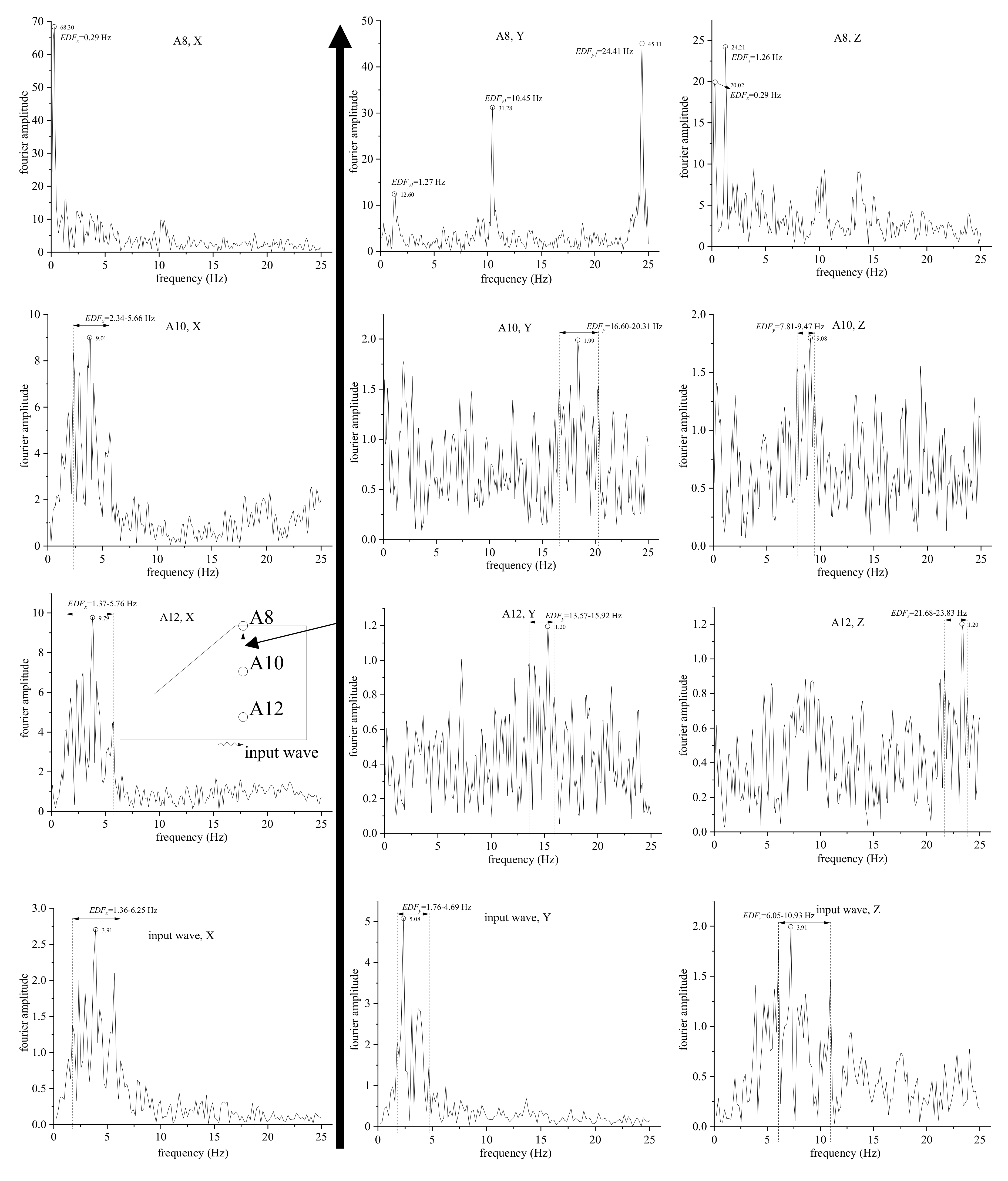
The acceleration histories can be transformed into Fourier spectra by applying a fast Fourier transformation (FFT) algorithm to the data. The Fourier spectra allow certain features of the dynamic response of the slope to be readily visualized. We are specifically interested in the variation of the Fourier amplitude with frequency and the earthquake dominant frequency (EDF). Three points in a model with α = 50° and β = 70° were chosen for Fourier analysis (A8, A10, and A12 along profile 2). Figure 10 shows the resulting Fourier spectra together with the corresponding ones generated for the input seismic wave. (The data in Figure 10 are arranged to emphasize how the form of the seismic vibration changes as it migrates upwards from the input level to points A12, A10, and then A8.)
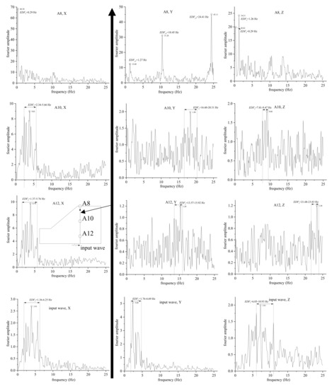
Figure 10.
Fourier spectra components and their dominant frequencies at different elevations within a slope subjected to the action of a natural seismic wave. The data are arranged in order of increasing elevation from bottom to top (points A12, A10, and A8 along profile 2).
Consider first the component of the Fourier spectrum in the X-direction. As can be seen, the EDF and amplitude of the Fourier spectrum in the X-direction vary little from the bottom of the slope (point A12) up to point A10: the former remains around 1–6 Hz and the latter remains around 9. However, as we move up to point A8, the Fourier amplitude is sharply amplified to 68.3 and the EDF is reduced to 0.29 Hz.
In the Y-direction, the EDF of the Fourier spectrum gradually increases as the input wave migrates to A10 while the Fourier amplitude slightly decreases. At point A8, however, the EDF shows double- or even triple-peak characteristics and the Fourier amplitude of the seismic component around 10 Hz is amplified to about 32. Moreover, the low frequency part (~1.27 Hz) is also amplified. The EDF of the Fourier spectrum in the Z-direction seems to decrease from bottom to top and reaches a minimum value of 1.2 Hz at point A8 (top of the slope). The Fourier amplitude essentially just fluctuates between 1.2 and 2.
In the planar problem, the Y- and Z-directions are equivalent to the horizontal and vertical directions, respectively. It is not surprising, therefore, that the patterns of Fourier amplitude variation found in these two directions are similar to the results obtained in previous table-shaking experiments [26]. On the whole, the seismic wave propagates from the bottom of the slope to the upper parts through reflection and refraction at the structural planes. The superposition effect of the seismic waves leads to the displacement response of the slope and hence relative motion of the rock masses. The more work that is conducted, the greater the amount of energy dissipation that will take place. As a result, high-frequency seismic waves with higher energy are generally more strongly attenuated and the EDF decreases correspondingly. Therefore, the dynamic response of the anti-dip bedding rock slope is stronger (and so more likely to become unstable) under the action of low-frequency seismic waves. This also explains why the AAFs of the slopes shown in Figure 7 are larger under the action of the sinusoidal wave (whose frequency is fixed at a low value of 5 Hz) than under the action of the natural seismic wave, (which contains frequency components that are much higher than 5 Hz).
4. Mechanism Responsible for Slope Failure under Seismic Action
The mechanism that leads to the failure of an anti-dip bedding rock slope subject to earthquake activity can be investigated by monitoring the displacement of the slope in the Y-direction as a function of time. Figure 11 presents contour plots of displacement data calculated for a slope with α = 40° and β = 60° by a cross parallel to the Y-axis through the center of the model. In the figure, the critical displacement value is taken to be 2 cm.
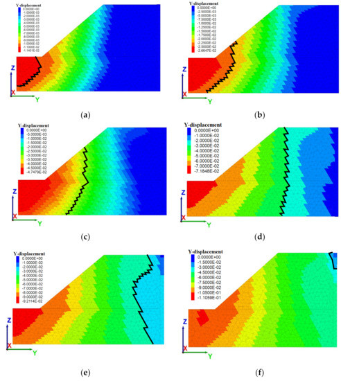
Figure 11.
Contour plots of the displacement in the Y-direction of a slope (α = 40° and β = 60°) subjected to a natural seismic wave. The plots show the displacements in the plane corresponding to x = 10 m at different times after the onset of the seismic disturbance: (a) 1 s, (b) 2 s, (c) 3 s, (d) 4 s, (e) 5 s, and (f) 6 s.
According to Figure 11, failure begins to occur under the seismic action at the leading edge of the slope. Furthermore, the failure surface is step-like, showing that the failure process has the characteristics of flexure toppling on the whole. As time progresses, a free surface is generated after the flexure toppling of the front edge and thus the rear part of the slope starts to undergo flexure toppling failure. The failure surface is therefore continuously extended to the rear part of the slope body. After the 5 s seismic loading wave had ended, the slope was already in a destabilized state. However, the slope displacement continued to develop beyond this point until the slope was completely destroyed.
These results should be compared with the results of shaking-table experiments conducted by previous authors [25]. In the current paper, it is found that the seismic wave induces the anti-dip bedding rock slope to start to fail at the bottom of the slope. In contrast, previous work has suggested that failure is due to the opening up of the structural planes at the top of the slope, which leads to the generation of tension cracks. It can thus be seen that the component of the seismic waves in the X-direction cannot be neglected. Furthermore, it is not just related to the stability of the anti-dip bedding rock slope, it also directly affects its failure mode.
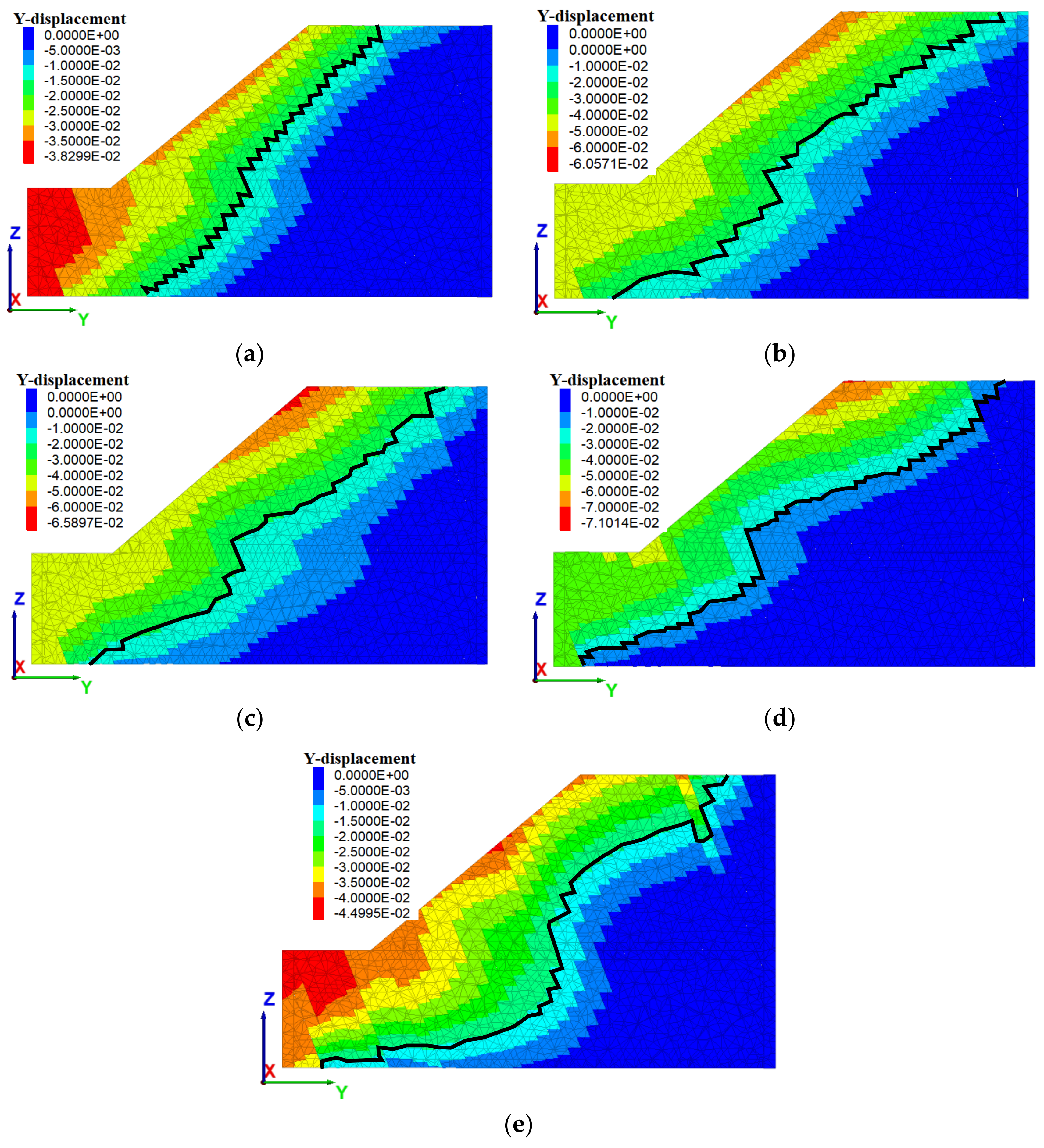
The influence of the spatial effect of the structural planes on the failure mode of the slope was also investigated. Figure 12 shows the displacement (again in the Y-direction) of a slope with α = 40° and β = 70° for different angles γ between the joint and slope trends. This time, the slope is subjected to the action of sinusoidal waves. In these plots, the critical displacement value is once again taken to be 2 cm. When γ = 0 (Figure 12a), the failure surface has a regular step-like shape. However, when γ ≠ 0, the failure surface becomes irregular.
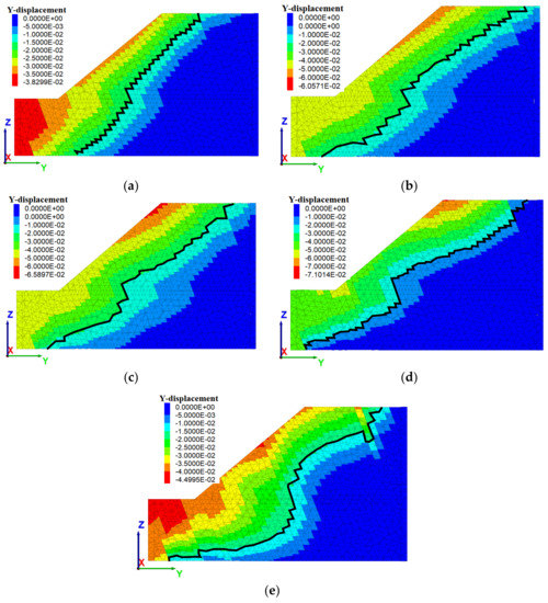
Figure 12.
Contour plots of the displacement in the Y-direction of a slope (α = 40° and β = 70°) subjected to a sinusoidal wave. The plots show the displacements in the plane corresponding to x = 10 m at the end of the period of disturbance (t = 5 s) for different values of γ: (a) 0°, (b) 5°, (c) 10°, (d) 15°, and (e) 20°.
It is also noticeable that, on the whole, the depth of the failure surface increases as the value of γ increases. At the same time, the scope of the slope instability becomes wider. Consequently, the slope will be less stable when subjected to dynamic action. When γ ≠ 0, the maximum displacement occurs around the upper shoulder of the slope, indicating that the most dangerous region of the slope (when it is subjected to dynamic action) is located in the upper part of the slope. Therefore, in areas of high seismic activity, it is essential that the statistics of the structural planes of an anti-dip bedding rock slope are thoroughly investigated before assessing the level of geological hazard present. This is because the spatial effects of the structural planes will directly affect the stability of the slope when it is subjected to seismic action.
5. Permanent Displacement of the Slope
5.1. Newmark’s Method
Some time ago, Newmark proposed an analysis method for dam slopes in which the stability of the slope under seismic action depends only on the permanent displacements it undergoes [27]. A pseudo-static method was subsequently used to derive an expression for the permanent displacement assuming the geotechnical object acts as a rigid body. Newmark thus found that the permanent displacement D only depends on the action of the seismic waves and safety factor of the slope under static forces. Based on this, an expression can be derived for D of the form,
where is the acceleration history and Ng is the horizontal critical acceleration, calculated using:
where is the slope angle and is the safety factor of the slope under static conditions. Newmark’s method is simple and easy to use. Other researchers have subsequently modified and improved the method and applied it to evaluate the stability of slopes and landslides [28,29].
As Newmark’s method can only consider the acceleration history in a single direction, in this work (for the sake of convenience later), the E–W direction of the Wolong seismic waves was selected for analysis purposes. This corresponds to the slope direction of displacement (i.e., the Y-axis). Furthermore, the displacement data for monitoring point D6 on the slope were chosen for analysis. Nine models were analyzed in all (Table 2).
Table 2.
Model-related parameters and permanent displacements calculated using Newmark’s method.
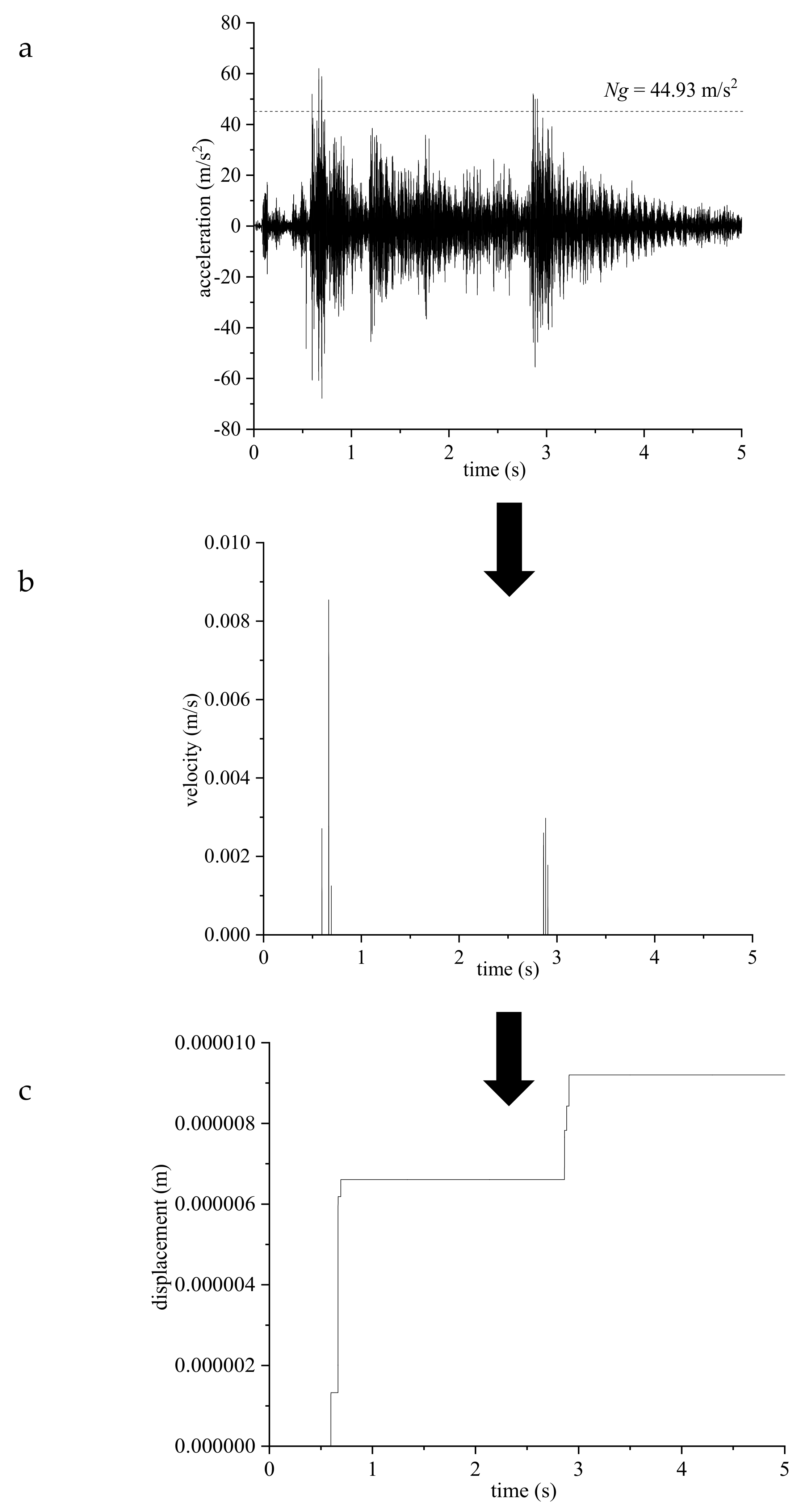
The SF values in the table were obtained via limit equilibrium analysis. Figure 13 illustrates the process used to find the permanent displacement using Newmark’s method (taking model No. 2 as an example). The permanent displacements thus obtained for each model are also shown in Table 2. It can be seen that the permanent displacement of the slope D tends to increase as the values of α and β increase. However, changing the angle α exerts a stronger influence compared to changing β because the surface of the slope is a free surface. Thus, the slope’s dip angle is inevitably the most important factor determining the displacement of individual points on the surface. In addition, the larger the joint angle β, the larger the topping moment and hence the lower the stability. Therefore, a larger permanent displacement will occur. The largest permanent displacement, 0.76 cm, occurred in the slope with α = 50° and β = 70°; the smallest, 0.0003 cm, in the slope with α = 40° and β = 50°.
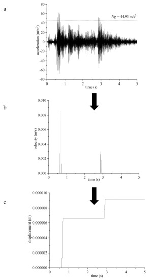
Figure 13.
Example of the use of Newmark’s method: (a) acceleration history (Y-direction) at point A6, (b) corresponding relative velocity history, and (c) cumulative displacement history.
5.2. Displacements Calculated Using the 3D Discrete-Element Method
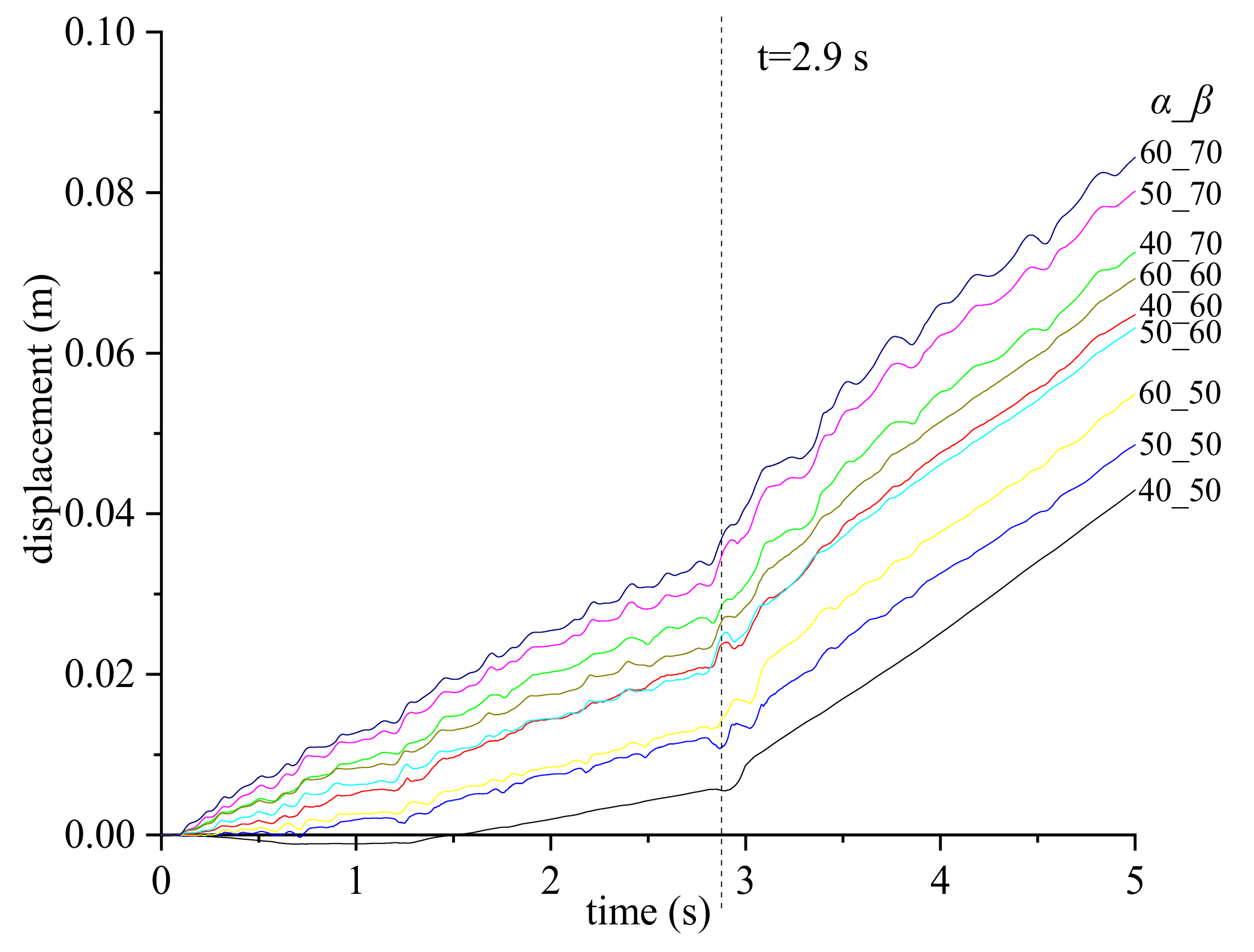
The permanent displacements of the slopes can also be obtained using the dynamic 3D discrete-element method. The monitoring point D5 was selected for this purpose. Figure 14 shows the displacement histories of the nine slopes listed in Table 2 (in the Y-direction at point D5) when the slopes are subject to the natural seismic wave.
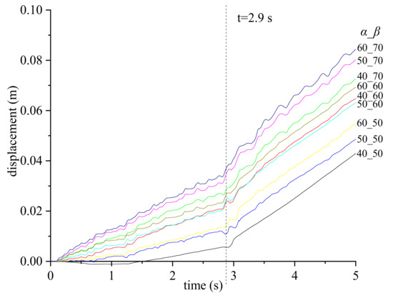
Figure 14.
Displacement history of point D5 in the Y-direction for different slopes subjected to the action of a natural seismic wave. The slopes are labeled α_β according to their α and β angles.
The results shown in Figure 14 imply that the displacement histories of each of the nine slopes do not converge, i.e., the slopes all become unstable. Moreover, there appears to be a critical time in the displacement histories Tc that occurs at ~2.9 s. Before Tc, the displacement at point D5 increases relatively slowly and so the curves have small gradients. After Tc, however, the rate of displacement suddenly becomes much faster (larger gradients), which means that the slopes experience accelerated rates of destabilization. Figure 14 also shows that the magnitudes of the slope displacements increase as the values of α and β increase. However, both α and β seem to have a similar degree of influence.
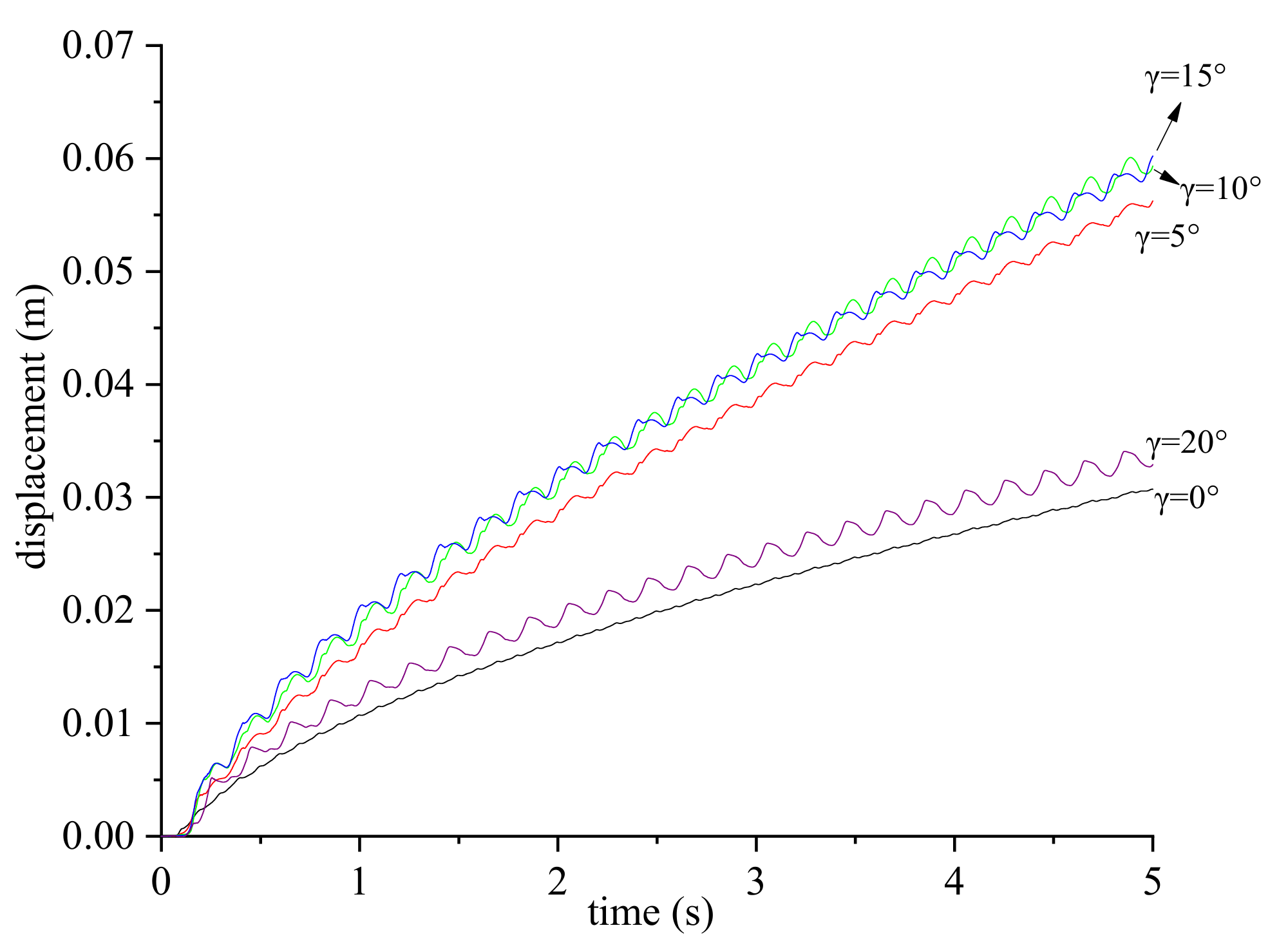
The effect of varying the angle γ on the permanent displacement of the slope was also studied (Figure 15). In this case, the sinusoidal wave was applied to one particular slope (with α = 40° and β = 70°) and the angle γ between the joint and slope trends was varied from 0° to 20°. The displacement history at point D5 in the Y-direction was then calculated while the wave was applied.
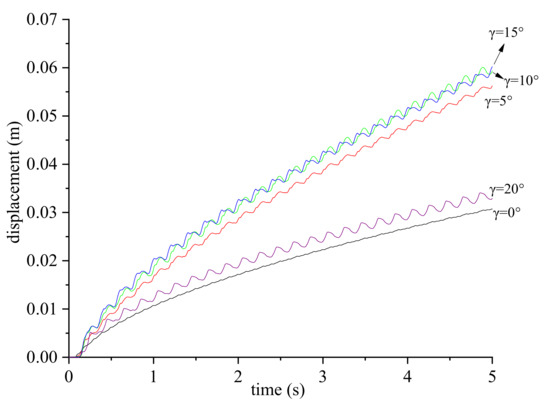
Figure 15.
Displacement history of point D5 in the Y-direction for slopes subjected to the action of a sinusoidal wave. Each slope has α = 40° and β = 70° but different values of γ.
As can be seen from Figure 15, the displacement at D5 under the action of the sinusoidal wave develops uniformly with time. That is, the displacement curves do not feature a critical time, Tc, similar to that shown in Figure 14. With the loading of the sinusoidal wave, the displacement exhibits an ‘S’ type fluctuation, that is, the local parts of the displacement history decrease and then increase. As γ is increased, the permanent displacement tends to increase at first and then decrease. When γ is increased from 15° to 20°, the permanent displacement decreases sharply and is very similar to that produced when γ = 0°. This regularity exactly matches that found in Section 3.1 (i.e., the way in which the acceleration amplification coefficient in the Y-direction varies with γ).
5.3. Comparison of Results and Discussion
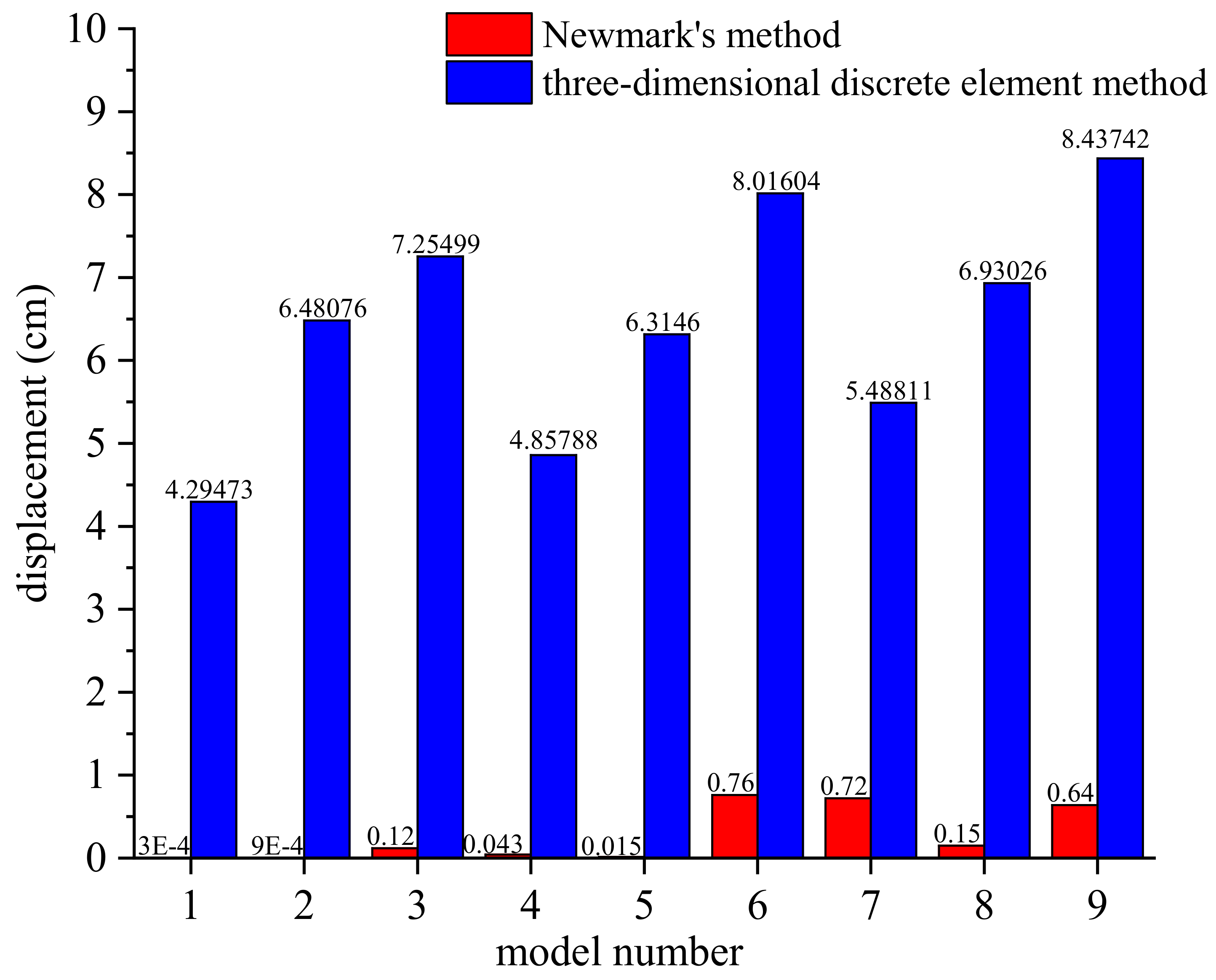
The permanent displacement of point D5 in the Y-direction has thus been found for different slopes using Newmark’s method and the 3D discrete-element method. It is instructive, therefore, to compare these results (Figure 16).

Figure 16.
Comparison of the permanent displacements of point D5 (in the Y-direction) under the action of a natural seismic wave as calculated using Newmark’s method and dynamic 3D discrete-element method.
The comparison shown in Figure 16 highlights the fact that the permanent displacements derived using Newmark’s method are significantly smaller than those obtained using the 3D discrete-element method. In fact, the largest differences between the two sets of predictions correspond to four orders of magnitude (models 1 and 2)—even the best correspondence amounts to an order of magnitude difference (model 7). Xiao et al. [30] also compared their results obtained for cascading landslides using a 2D discrete-element method (UDEC) with those obtained using Newmark’s method and found better correspondence. However, in contrast to the comparative study conducted by Xiao et al., we have conducted a comparison between the 3D discrete-element method and Newmark’s method of anti-dip bedding rock slopes by permanent displacement. Therefore, the results obtained in this paper are the product of a more comprehensive analysis. That is, we took into account the following factors:
- Compared with bedding slopes (or landslides), anti-dip bedding slopes are more stable under static conditions and have higher safety factors (SF). On the other hand, Newmark’s method is based on the assumption that sliding failure occurs with a straight failure surface. This is obviously contrary to the flexure toppling failure mode of anti-dip bedding rock slopes.
- Newmark’s method is based on a pseudo-static method and assumes that the geotechnical object can be regarded as a rigid, nondeforming body. In reality, the geotechnical object will deform and the 3D discrete-element method takes this into account. As a result, the displacement obtained using our method will be larger.
- Newmark’s method is based on the assumption that the problem can be treated in a single plane; the seismic waves and displacements are also considered to be in the same horizontal direction. In this paper, we consider the loading caused by the seismic waves in the X-, Y- and Z-directions. This means our model can account for 3D spatial effects that cannot be treated using a simple single-plane approach.
In summary, although Newmark’s method is simple and easy to operate, it cannot be used to objectively and accurately determine the permanent displacement of anti-dip bedding slopes subject to 3D seismic loading (and hence their stability). Instead, a more mature and complex analysis method needs to be used.
6. Conclusions
In this paper, 3D discrete-element numerical software (3DEC) is used to analyze the dynamic response and failure mechanism of anti-dip bedding rock slopes with different slope angles, joint angles, and angles between the joint and slope trends. The slopes were subjected to the action of natural seismic waves and sinusoidal waves loaded in three directions. The permanent displacement of the slope was also calculated using Newmark’s method. The following conclusions can be drawn:
- When the slope is dynamically loaded using a 3D seismic wave, the 3D acceleration magnification coefficient of the slope is not very regular; there is also no sign of obvious ‘elevation’ and ‘appearance’ effects. Instead, it shows rhythmicity. The peak acceleration amplification effect is more significant under the action of sinusoidal waves. As the angle between the joint and slope trends increases, the amplification effect of the slope first decreases and then increases.
- As the seismic wave propagates within the slope, the amplitudes of the low-frequency parts of the seismic wave are generally amplified and the earthquake dominant frequency tends to decrease. The EDF in the Y-direction also diverges, forming 2 or 3 peaks.
- When subjected to seismic action, the slope starts to fail in the lower part of the slope and failure progresses from bottom to top. The failure surface is step-like, showing the characteristics of flexure toppling. When the angle between the joint and slope trends is nonzero, the failure surface becomes more irregular. Moreover, as this angle increases, the depth of the failure surface increases and the scope of the unstable part of the slope becomes wider.
- The permanent displacement of the slope increases as the slope and joint angles increase. Under the action of natural seismic waves, the displacement of the slope in the Y-direction develops slowly at first and then accelerates at a critical time Tc. As the angle between the joint and slope trends increases, the permanent displacement of the slope increases and then decreases.
- Newmark’s method only considers the action of seismic waves in one direction (i.e., the method is only useful for planar problems). The displacement results obtained using the method are much smaller than those obtained using the dynamic 3D discrete-element method. The results obtained using Newmark’s method are therefore overly conservative.
Author Contributions
Conceptualization and methodology, C.C. and C.S.; Data curation, Y.W.; Software, Z.R. and C.S.; Writing—original draft, Z.R.; Writing—review and editing, Z.R. and C.S. All authors have read and agreed to the published version of the manuscript.
Funding
The research was financially supported by National Natural Science Foundation of China (Grant Nos. 12072358 and 12102443). We are grateful for the Foundation’s continued support and also to our colleagues for their valuable help to this research.
Conflicts of Interest
The authors declare that there are no conflict with this publication.
References
- Goodman, R.E.; Bray, J.W. Toppling of Rock Slopes. In Proceedings of the Specialty Conference on Rock Engineering for Foundations and Slopes, Boulder, CO, USA, 15–18 August 1976; Volume 2, pp. 201–234. [Google Scholar]
- Aydan, Ö.; Kawamoto, T. The stability of slopes and underground openings against flexural toppling and their stabilisation. Rock Mech. Rock Eng. 1992, 25, 143–165. [Google Scholar] [CrossRef]
- Liu, C.H.; Jaksa, M.B.; Meyers, A.G. Improved analytical solution for toppling stability analysis of rock slopes. Int. J. Rock Mech. Min. Sci. 2008, 45, 1361–1372. [Google Scholar] [CrossRef]
- Zheng, Y.; Chen, C.; Liu, T.; Zhang, H.; Sun, C. Theoretical and numerical study on the block-flexure toppling failure of rock slopes. Eng. Geol. 2019, 263, 105309. [Google Scholar] [CrossRef]
- Ding, B.; Han, Z.; Zhang, G.; Beng, X.; Yang, Y. Flexural Toppling Mechanism and Stability Analysis of an Anti-dip Rock Slope. Rock Mech. Rock Eng. 2021, 54, 3721–3735. [Google Scholar] [CrossRef]
- Alejano, L.R.; Gómez-Márquez, I.; Martínez-Alegría, R. Analysis of a complex toppling-circular slope failure. Eng. Geol. 2010, 114, 93–104. [Google Scholar] [CrossRef]
- Brideau, M.A.; Stead, D. Controls on block toppling using a three-dimensional distinct element approach. Rock Mech. Rock Eng. 2010, 43, 241–260. [Google Scholar] [CrossRef]
- Xue, Y.; Kong, F.; Yang, W.; Qiu, D.; Su, M.; Fu, K.; Ma, X. Main unfavorable geological conditions and engineering geological problems along Sichuan-Tibet railway. Chin. J. Rock Mech. Eng. 2020, 39, 445–468. [Google Scholar]
- Peng, J.B.; Cui, P.; Zhuang, J.Q. Challenges to engineering geology of Sichuan-Tibet railway. Chin. J. Rock Mech. Eng. 2020, 39, 2377–2389. [Google Scholar]
- Chinese Code GB 50011-2010, Code for Seismic Design of Buildings. Available online: https://www.doc88.com/p-3037442363978.html (accessed on 31 August 2018).
- Yagoda, B.G.; Hatzor, Y.H. A new failure mode chart for toppling and sliding with consideration of earthquake inertia force. In Proceedings of the 47th US Rock Mechanics/Geomechanics Symposium, San Francisco, CA, USA, 23–26 June 2013. [Google Scholar]
- Guo, S.; Qi, S.; Yang, G.; Zhang, S.; Saroglou, C. An analytical solution for block toppling failure of rock slopes during an earthquake. Appl. Sci. 2017, 7, 1008. [Google Scholar] [CrossRef]
- Zheng, Y.; Chen, C.; Liu, T.; Ren, Z. A new method of assessing the stability of anti-dip bedding rock slopes subjected to earthquake. Bull. Eng. Geol. Environ. 2021, 80, 3693–3710. [Google Scholar] [CrossRef]
- Fan, G.; Zhang, J.; Wu, J.; Yan, K. Dynamic response and dynamic failure mode of a weak intercalated rock slope using a shaking table. Rock Mech. Rock Eng. 2016, 49, 3243–3256. [Google Scholar] [CrossRef]
- Chen, C.-C.; Li, H.-H.; Chiu, Y.-C.; Tsai, Y.-K. Dynamic response of a physical anti-dip rock slope model revealed by shaking table tests. Eng. Geol. 2020, 277, 105772. [Google Scholar] [CrossRef]
- Ning, Y.; Zhang, G.; Tang, H.; Shen, W.; Shen, P. Process analysis of toppling failure on anti-dip rock slopes under seismic load in southwest China. Rock Mech. Rock Eng. 2019, 52, 4439–4455. [Google Scholar] [CrossRef]
- Zhang, Z.; Wang, T.; Wu, S.; Tang, H. Rock toppling failure mode influenced by local response to earthquakes. Bull. Eng. Geol. Environ. 2016, 75, 1361–1375. [Google Scholar] [CrossRef]
- Fan, G.; Zhang, L.; Zhang, J.; Yang, C. Analysis of seismic stability of an obsequent rock slope using time–frequency method. Rock Mech. Rock Eng. 2019, 52, 3809–3823. [Google Scholar] [CrossRef]
- Zheng, Y.; Wang, R.; Chen, C.; Sun, C.; Ren, Z.; Zhang, W. Dynamic analysis of anti-dip bedding rock slopes reinforced by pre-stressed cables using discrete element method. Eng. Anal. Bound. Elem. 2021, 130, 79–93. [Google Scholar] [CrossRef]
- Itasca 3DEC-3 Dimensional Distinct Element Code, Version 5.2; Itasca Consulting Group: Minneapolis, MN, USA, 2019.
- Kuhlemeyer, R.L.; Lysmer, J. Finite element method accuracy for wave propagation problems. J. Soil Mech. Found. Div. ASCE 1973, 99, 421–427. [Google Scholar] [CrossRef]
- Chinese Code GB/T 17742-2020, The Chinese Seismic Intensity Scale. Available online: https://www.doc88.com/p-61773129398077.html (accessed on 27 August 2020).
- Rizzitano, S.; Cascone, E.; Biondi, G. Coupling of topographic and stratigraphic effects on seismic response of slopes through 2D linear and equivalent linear analyses. Soil Dyn. Earthq. Eng. 2014, 67, 66–84. [Google Scholar] [CrossRef]
- Yang, G.; Qi, S.; Wu, F.; Zhan, Z. Seismic amplification of the anti-dip rock slope and deformation characteristics: A large-scale shaking table test. Soil Dyn. Earthq. Eng. 2018, 115, 907–916. [Google Scholar] [CrossRef]
- Yang, G.; Ye, H.; Wu, F.; Qi, S.; Dong, J. Shaking table model test on dynamic response characteristics and failure mechanism of antidip layered rock slope. Chin. J. Rock Mech. Eng. 2012, 31, 2214–2221. [Google Scholar]
- Fan, G.; Zhang, J.J.; Fu, X. Dynamic response differences between bedding and count-tilt rock slopes with siltized intercalation. Chin. J. Geotech. Eng. 2015, 37, 692–699. [Google Scholar]
- Newmark, N.M. Effects of earthquakes on dams and embankments. Geotech. 1965, 15, 139–160. [Google Scholar] [CrossRef] [Green Version]
- Jibson, R.W. Predicting earthquake-induced landslide displacements using Newmark’s sliding block analysis. Transp. Res. Record 1993, 1411, 9–17. [Google Scholar]
- Romeo, R. Seismically induced landslide displacements: A predictive model. Eng. Geol. 2000, 58, 337–351. [Google Scholar] [CrossRef]
- Xiao, K.; Li, H.; Liu, Y.; Xia, X.; Zhang, L. Study on deformation characteristics of bedding slopes under earthquake. Rock Soil Mech. 2007, 28, 1557–1564. (In Chinese) [Google Scholar]


Publisher’s Note: MDPI stays neutral with regard to jurisdictional claims in published maps and institutional affiliations. |
© 2022 by the authors. Licensee MDPI, Basel, Switzerland. This article is an open access article distributed under the terms and conditions of the Creative Commons Attribution (CC BY) license (https://creativecommons.org/licenses/by/4.0/).