Abstract
With the development and popularization of unmanned aerial vehicles (UAVs) and surveillance cameras, vehicle re-identification (ReID) task plays an important role in the field of urban safety. The biggest challenge in the field of vehicle ReID is how to robustly learn the common visual representation of vehicle from different viewpoints while discriminate different vehicles with similar visual appearance. In order to solve this problem, this paper designs the normalized virtual softmax loss to enlarge the inter-class distance and decrease the intra-class distance, and a vehicle ReID model is proposed by jointly training the network with the proposed loss and triplet loss. In addition, we contribute a novel UAV vehicle ReID dataset from multiple viewpoint images to verify the robustness of methods. The experimental results show that comparing with the other softmax-based losses, our method achieves better performance and gets 76.70% and 98.95% in Rank-1 on VRAI and VRAI_AIR dataset, respectively.
1. Introduction
With the development of economy, public safety is attracting more and more attention in society. As the most commonly used transportation, vehicles may be related to criminal activities, in which accurately locating the vehicles in surveillance system is the key to stopping crime and keeping the city safe. However, the license plates of the suspect vehicles are often taken down, replaced or blocked, making troubles in locating them by plates. Thus, the vehicle re-identification (ReID) technology that distinguishes vehicles by visual features has been developed and plays an important role in urban governance [1], anti-terrorist attacks [2] and tracking criminals [3].
The unmanned aerial vehicles (UAVs) are developing rapidly, research on images of which has gradually draw an increasing attention by both academia and industry that yet focus on object detection and target tracking task mostly. In vehicle ReID task, the disadvantages of traffic surveillance cameras is that it has fixed locations and limited viewpoints. In contrast, the UAV platform gets broader range of perspectives and large-scale scene, as well as better flexibility, mobility and convenience.
In spite of the great research value, there are intractable problems in vehicle ReID task on UAV platform.
- Datasets: according to our survey results, vehicle ReID from UAV platform is a less explored task, and there is a lack of public dataset. Most of the vehicle ReID datasets are derived from urban surveillance systems of which images are very different from those got by UAV (shown in Figure 1a,c), and the existing UAV image datasets originally serve object detection or target tracking task in which camera’s height is too high to get a suitable spatial resolution for ReID task (shown in Figure 1b). As far as we are concerned, the only UAV platform dataset especially for the vehicle ReID task is VRAI [4] and it’s difficult to comprehensively examine the effectiveness of the algorithms using one single dataset for research. The scarcity of the dataset restricts the research on vehicle ReID on UAV platforms.
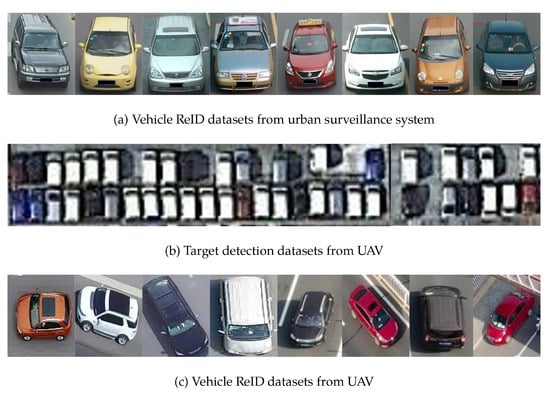 Figure 1. Different datasets for different tasks and captured by different platform.
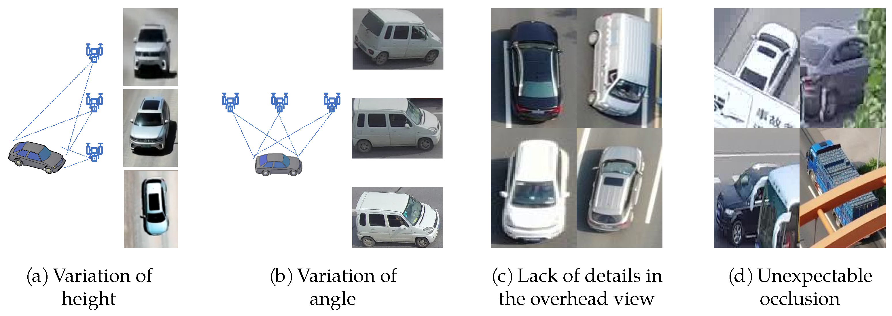
 - Viewpoint: the image features of the UAV platform are very different from that of the fixed surveillance cameras. Fixed surveillance cameras are installed in the well-chosen location along the streets so that the discriminative visual features behind the windshield can be easily found, and there is little occlusion in the pictures. The UAV moves relatively flexible, having a wide range of height changes (3~100 m) and angle changes (pitch angle ~, yaw angle ~) (Figure 2a,b), and less detailed visual features at large angle of inclination (Figure 2c). What’s more, the image spatial resolution is relatively reduced and there is unpredictable occlusion during the flying (Figure 2d).
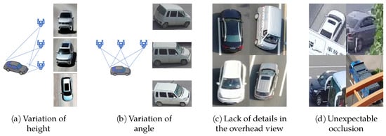 Figure 2. The problem of viewpoint in vehicle ReID on UAV platform.
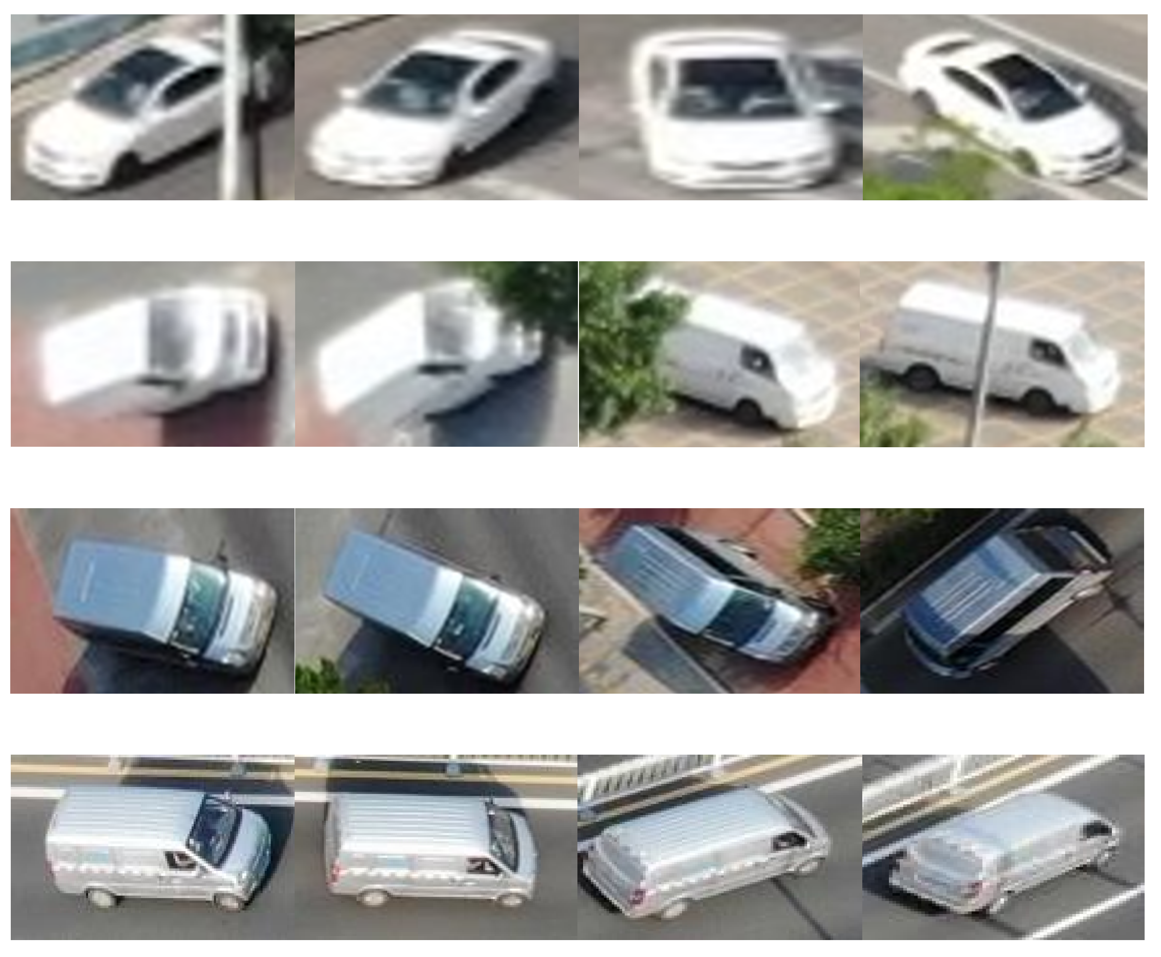
 - Confusion: the image features of the UAV platform exacerbated the problem of large intra-class difference and small inter-class difference. There are three major challenges in Vehicle ReID task. Firstly, the number of classes is very large. Researchers often use classification loss when training the network in the vehicle ReID task, which means every unique vehicle (every ID) is treated as an independent class. For example, there are 13,021 classes in VRAI dataset, while there are only 80 classes in Microsoft Common Objects in Context dataset (COCO) [5], which is a famous target detection and segmentation dataset. Secondly, the intra-class difference is large. The same car under the different cameras at variations in viewpoints, altitudes, and under different illuminations may seem completely different. Figure 3a shows two examples. Thirdly, the inter-class difference is tiny. Different vehicles with same brand or same paint may seem of no difference, which can only be distinguished by discriminative visual details. Figure 3b shows four different vehicles with same paint. The problem of viewpoint aggravates the confusion of inter-class and intra-class and the confusion is relative to the mixture of features among different classes in feature space.
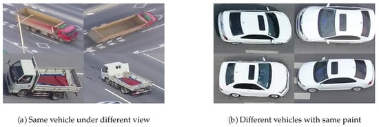 Figure 3. Intra-class variation and inter-class similarity in the vehicle ReID.
Typically, a standard ReID system contains two main components: feature extraction and metric learning [6,7,8]. The former focus on extracting clear features from images and the latter concentrates on optimizing the feature distance in feature space. Recently most of the researchers are attracted to the proposal of novel feature extraction networks, leaving the metric learning with barely research. However, the problems of UAV vehicle ReID mentioned above are just relative to the phenomenon of mixed feature space and the weakness of the metric learning ability. Thus, we introduce joint normalized virtual softmax loss (NV-softmax loss) and triplet loss to guide a better feature distance learning. In the practical application of vehicle ReID technology, comparing with the other softmax-base method, ours can return more accurate query results, thus effectively identifying criminal vehicles.
In summary, vehicle ReID task on UAV platform involves many new challenges and difficulties, which requires detailed discrimination ability. In this paper, we build a new UAV dataset called VRAI-AIR to provide effective data support for complex backgrounds and various viewpoints of UAV images. Furthermore, we design normalized virtual softmax loss with triplet loss to solve viewpoint and confusion problem. We will elaborate in the latter two sections of Dataset and Method.
2. Related Work
2.1. Dataset
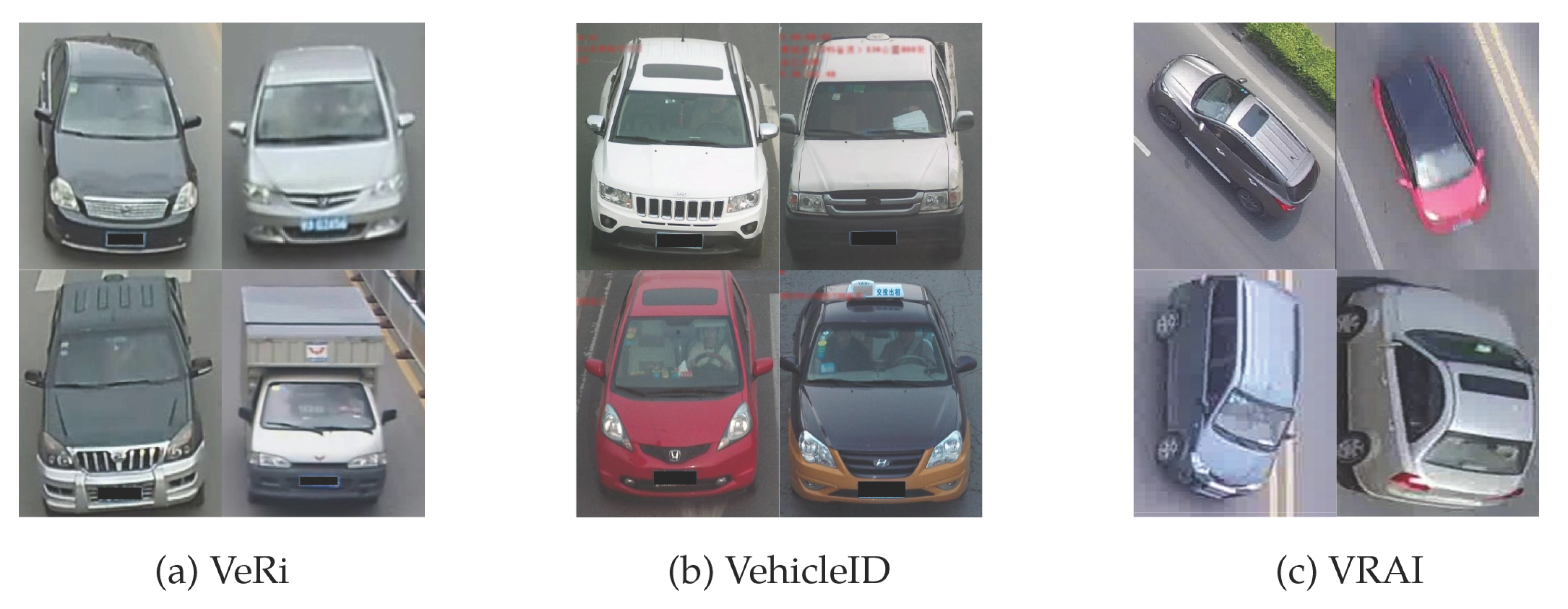
There are several established benchmark datasets for Vehicle ReID task. VeRi [9] (Figure 4a) is a relatively small dataset including 40,000 bounding boxes of 619 vehicles. The advantage of VeRi is that the location of cameras is showed on the map and the distance between them is showed in a matrix so researcher can take spatio-temporal relationship into account. VehicleID [10] (Figure 4b) is a much larger dataset with 221,763 images of 26,267 vehicles, and the license plate of the vehicles is especially made to be mosaic to better suit the real usage of vehicle ReID task.

Figure 4.
Samples from different datasets.
With the rapid development of UAVs, some aerial remote sensing visual datasets were constructed for the research on UAV vision tasks, among which DOTA and VisDrone have received special attention. DOTA [11] is a large-scale remote sensing dataset, part of which comes from UAVs while the other part from satellites. The images from the UAVs aim to serve the object detection task so the flying height is so high that the spatial resolution is not suitable for the ReID task. VisDrone dataset [12] consists of 400 video clips formed by 265,288 frames and 10,209 static images, which is used as the benchmark for the challenge of “vision meets drone”. VisDrone is used for object detection and tracking, but the images with higher spatial resolution have the probability to evaluate ReID task if further annotation can be labeled.
Considering that the lack of UAV dataset limits the research of Vehicle ReID task on UAV platform, Wang et al. [4] constructed an aerial dataset called VRAI (Vehicle Re-identification in Aerial Imagery, Figure 4c). VRAI are captured by two DIJ consumer UAVs at different location with a diversified shooting angles and flight altitudes, including 137,613 images of 13,022 vehicles, and 66,113 images among them are published. There is something special about VRAI that the discriminative parts of vehicles are marked by the bounding box, such as luggage racks and personalized stickers. However, high image resolution of the dataset with large memory size is not suitable for practical application, and one single dataset cannot effectively test the robustness of algorithm, so we come up with our own dataset.
2.2. Vehicle ReID Approaches
Ye et al. [6] roughly divide the ReID task into two parts—feature representation and metric learning. Feature representation focuses on constructing different networks to extract features from images, while metric learning focuses on designing different loss functions, and related work is also carried out around these two points.
In terms of feature representation, most existing works adopt the network designed for classification task as the backbone, in which every unique vehicle (every ID) is treated as a class. Resnet [13] is widely used and has been proven to be the best backbone, in which a deep residual learning framework is proposed to solve the problem of degradation. Furthermore, for the first few layers of the convolutional neural network (CNN) only extract the dataset-independent texture information [14], Resnet is often pre-trained on the large dataset ImageNet [15] to get general learning capabilities for better performance. Based on Resnet, Wang et al. [4] proposed a ReID method adapted to the characteristics of the VRAI dataset. On the one hand, they use deep CNN to extract global features of every image, and on the other hand, they use an object detector to detect discriminative parts, and finally combine the features of discriminative parts with global features to get the weighted features. With the popularity of the visual transformer (ViT) [16], He et al. [17] applied it to the ReID task and also achieved good performance.
In terms of metric learning, Boltzmann [18] proposes the softmax function in 1868. Gibbs [19] standardizes the specific form of softmax. John S. Bridle [20] firstly use softmax for pattern recognition. Lu Chenguang [21] and Rubinstein [22] propose cross-entropy, respectively. Softmax is combined with cross-entropy to form the cross-entropy loss, or softmax loss. It is also called classification loss because often used in classification problems. Zheng et al. [23] apply classification loss to the ReID problems and thus it is also called ID loss. The drawback of the original classification loss is that it cannot solve the problem of large intra-class differences and small inter-class differences, so some improvement methods are proposed. Liu et al. [24] apply large-margin softmax (L-softmax) to CNN to compressed the angle of the feature space occupied by each class in the orignal softmax to 1/m. Based on L-softmax, angular softmax (A-softmax) [25] proposed by Liu et al. normalizes the fully connected matrix and sets the bias of the fully connected layer to 0, so that the high-dimensional feature vectors of the images are mapped on a hypersphere of radius 1 in the feature space.
L-softmax and A-softmax need to set hyperparameters and the computational complexity is large. Chen et al. [26] propose the virtual label and apply it to target classification and face recognition, without any hyperparameters or significant increase of the computational complexity. By inserting each sample into the feature space as a dynamic virtual class during the training process, the virtual softmax compresses the intra-class differences and increases the inter-class differences.
Zheng et al. [27] propose the virtual labels in another sense for vehicle ReID. They divide the entire training process into two stages. In the stage I, four datasets of CityFlow, VehicleID, CompCar, and VeRi are simply merged into one data set called “VehicleNet”, on which a deep CNN network is trained with classification loss. In the stage II, only one specific dataset above all four datasets is used, and the fully-connected layer is replaced with an untrained one, leaving the feature extraction part of the network retained. In this way, the IDs of the other three datasets can be seen as the “virtual classes” to the specific dataset.
What’s more in the metric learning, Hermans et al. [28] think that using triplet loss may achieve a better performance than classification loss. Wang et al. [29] combine the triplet loss and the classification loss, which is a proven way to improve model performance. In addition, Luo et al. [30] propose the BNNeck to combine the triplet loss and ID loss. Zhong et al. [31] propose k-reciprocal re-ranking that re-query the results of the first query in the inference phase to achieve better performance.
3. Dataset
To solve the lack of datasets mentioned in the Introduction, we collect and annotate our own dataset and name it VRAI_AIR, which means vehicle re-identification in aerial imagery made by Aerospace Information Research Institute, Chinese Academy of Science.
To develop the diversity of the UAV-based vehicle ReID datasets, different from the DJI Phantom 4 for the VRAI dataset, we choose DJI Mavic Air 2 as the image acquisition platform, which has longer flight time, larger field of view and HDR (High Dynamic Range Imaging) mode.
We fly two DJI Mavic Air 2 drones along Huairou campus of UCAS for a long distance. The location is carefully chosen because the road is located in the suburban area with moderate traffic flow and vehicle speed which avoid blur and occlusion, containing a diversity of vehicle types such as trucks and lorries. We make the drones fly as long a distance as possible to simulate situations that might be encountered in a real deployment. There are trees, street signs and overpass on the road, and parking lot, pedestrian crosswalk, crossroads and no-parking area during the long-distance flight, which provides a convenience to capture images with complex background, as shown in Figure 5.
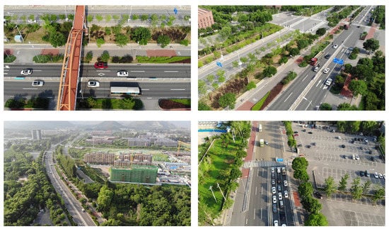
Figure 5.
Overlooking view of the shooting place.
During the flight, the drones work in the video mode of FHD HDR with 1920 × 1080 resolution and 30 fps, and the flight-altitude ranges from 30 m to 90 m. We control the drones to fly in various modes, including hovering, circling, following, rapid ascent, rapid descent, etc., while controlling the cameras to swing in order to get diverse images of vehicles.
After the flight, we obtain the videos captured by the drones. Considering the average speed of the vehicles and the frame rate of the videos, we took one frame from every four frames as the material for annotation, and get a total of 1304 panoramic images. We use LabelMe [32] to label the vehicles in panoramic images with axis-aligned bounding boxes. By aligning the real time of the two UAV videos and labeling them frame by frame, we are able to match vehicles with the same ID in different panoramic images with consistent labels. Furthermore, we count the images attributes to make better use of the dataset.
We obtain 1783 vehicle slices of 202 IDs in total, details shown in Figure 6. Each ID owns 8.8 images on average, the most owns 56 images, the least owns 2 images, and most of the IDs own between 3 and 12 images, the detailed Image/ID situation is shown in Figure 7a.

Figure 6.
Details of our dataset.
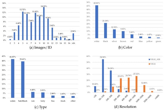
Figure 7.
Image attributes of VRAI_AIR.
Although our method does not use additional information for inference, we still labeled the dataset with additional information to facilitate the research of others, including colors and vehicle types. Regarding the color information, it is worth noting that (1) “gray” cars is categorized as “silver” cars because it is difficult to tell the difference between them; (2) for cases where the vehicle has more than one color (e.g., large spray paint and stickers), we only label the color that occupies the largest area of the body; (3) all colors are listed and no color is classified as “other”. The detailed statistics of the color information is shown in Figure 7b, from which it’s easy to see that the exterior color of the vehicle is mostly black, white and silver.
As for as the type information, it is worth noting that “sedan” refers to three compartments cars, “hatchback” refers to two compartments cars including SUV, “lorry” here refers to small trucks and “truck” here refers to large trucks, “other” often means some tool vehicles, such as concrete mixer trucks, etc. The detailed statistics of the car type information is shown in Figure 7c, it can be seen that, although we chose the non-urban road to shoot, but sedan and hatchback still account for the majority.
We also count the image resolution of the dataset and compare it with the VRAI dataset, and the resolution distribution of the two is shown in Figure 7d. It can be seen that the resolution of the images in our dataset is concentrated in the range of 5 K–20 K, while the resolution of the VRAI dataset is concentrated in a higher interval. The difference in resolution between the two datasets promotes the diversity of the UAV-based vehicle ReID datasets.
4. Method
In this section, we introduce the proposed loss function named normalized virtual softmax loss. In addition, compare the effects of the proposed loss function and the original softmax loss. Finally, we present the whole model jointly using the NV-softmax loss and triplet loss.
4.1. Normalized Virtual Softmax Loss
Softmax loss, also called classification loss, is often used in vehicle ReID task, in which every unique vehicle (every ID) is treated as a class. It can divide the different classes but cannot pull them apart, leading to the samples near the decision boundaries are often misclassified, which is not a big challenge in classification task but extremely exacerbates the performance of ReID network, due to the problems of mixed feature space mentioned in Introduction. The most effective method to solve the problem is to keep the samples as far away from the decision boundaries as possible, or just pull apart the decision boundaries of different classes, where a new loss function is called to be proposed.
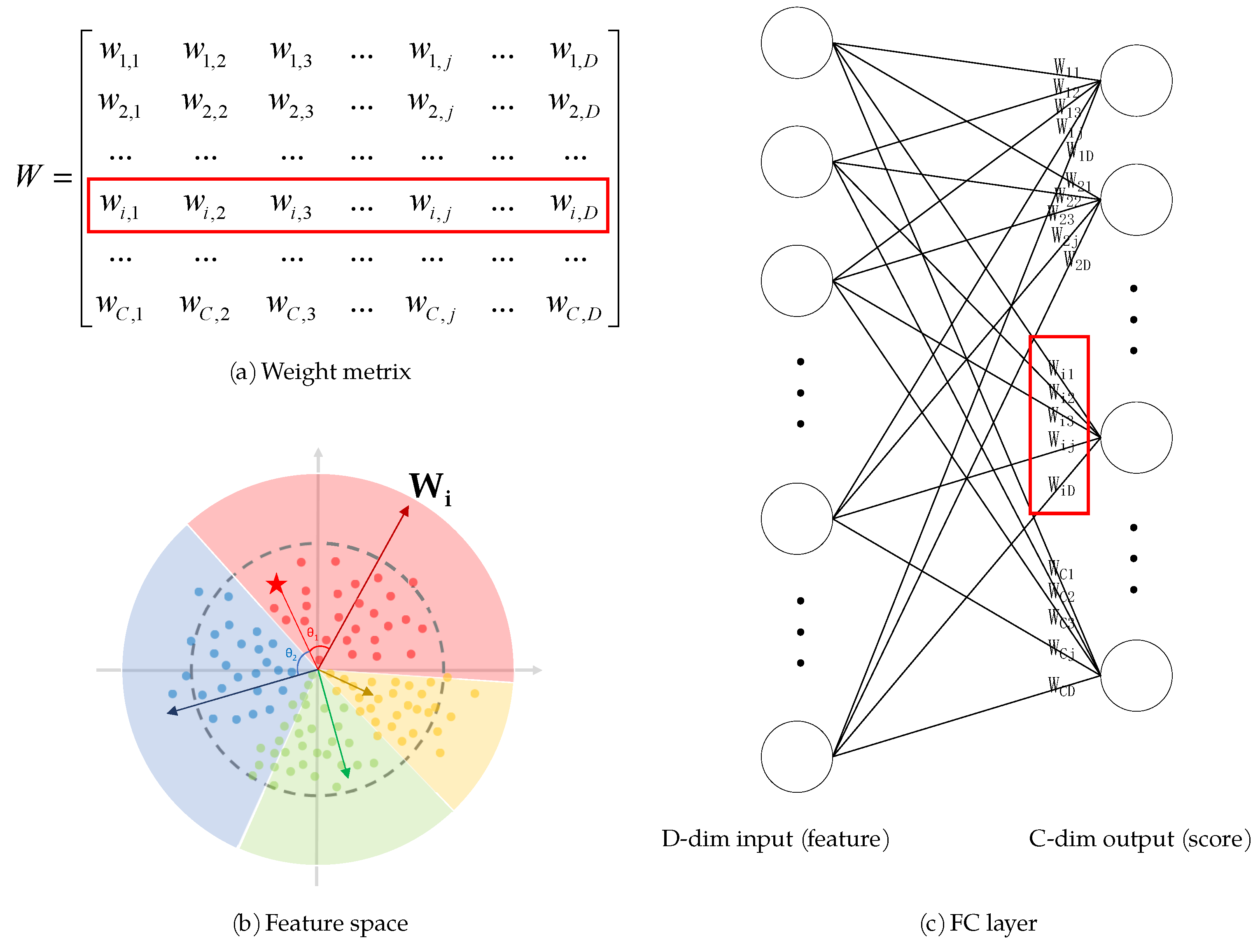
Softmax loss is a combination of fully connected layer, softmax function and cross-entropy loss. An image passes through feature extraction network, transformed to a D-dimensional vector X containing high-dimensional feature of the original image, and then enters into the last fully connected layer (FC layer) of the network to multiply with the weight matrix W. Each row vector of the weight matrix can be seen as the coordinates of each class’s central position in the feature space as perceived by the current network, which is called the class anchor (Equation (1)), as shown in Figure 8. So the multiplication between the feature vector and the row vector of weight matrix is essentially the calculation of the cosine similarity between them (Equation (2)). The calculate C similarities make up the score vector S corresponding to C classes (Equation (3)). In the inference stage, the class with the largest score is inferred by the network as the class to which the sample belongs. As an example of 2-class classification problem, shown in Figure 9a, sample is judged to be the red class when . In the training stage, the S is modified by softmax function to (Equation (4)), and calculated the cross-entropy loss L (Equation (6)) with the ground truth of the image in one-hot form (Equation (5)), where N is the batch size, k means the k-th sample in a batch and is the class anchor of the k-th sample’s ground truth.
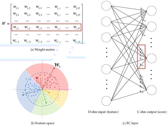
Figure 8.
The relationship among (a) the weight matrix, (b) the feature space and (c) the FC layer.
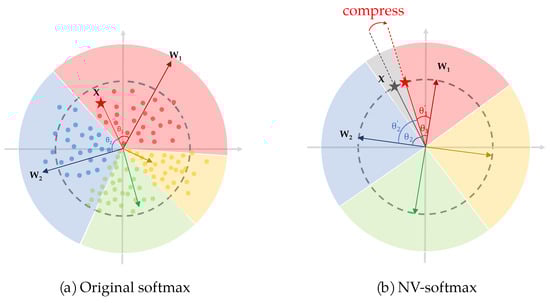
Figure 9.
The feature space of original softmax and normalized virtual softmax.
The loss back propagates (Equation (7)) to modify the parameters of the network to make the samples away from the boundaries and move closer to the anchor of the class they belonging to. The farther the samples are from the boundaries, the less likely the network is to misclassify. So, it is easy to come up with an idea to create some “no-man’s land” between two adjacent space to promote this process, which is the original purpose of the virtual class.
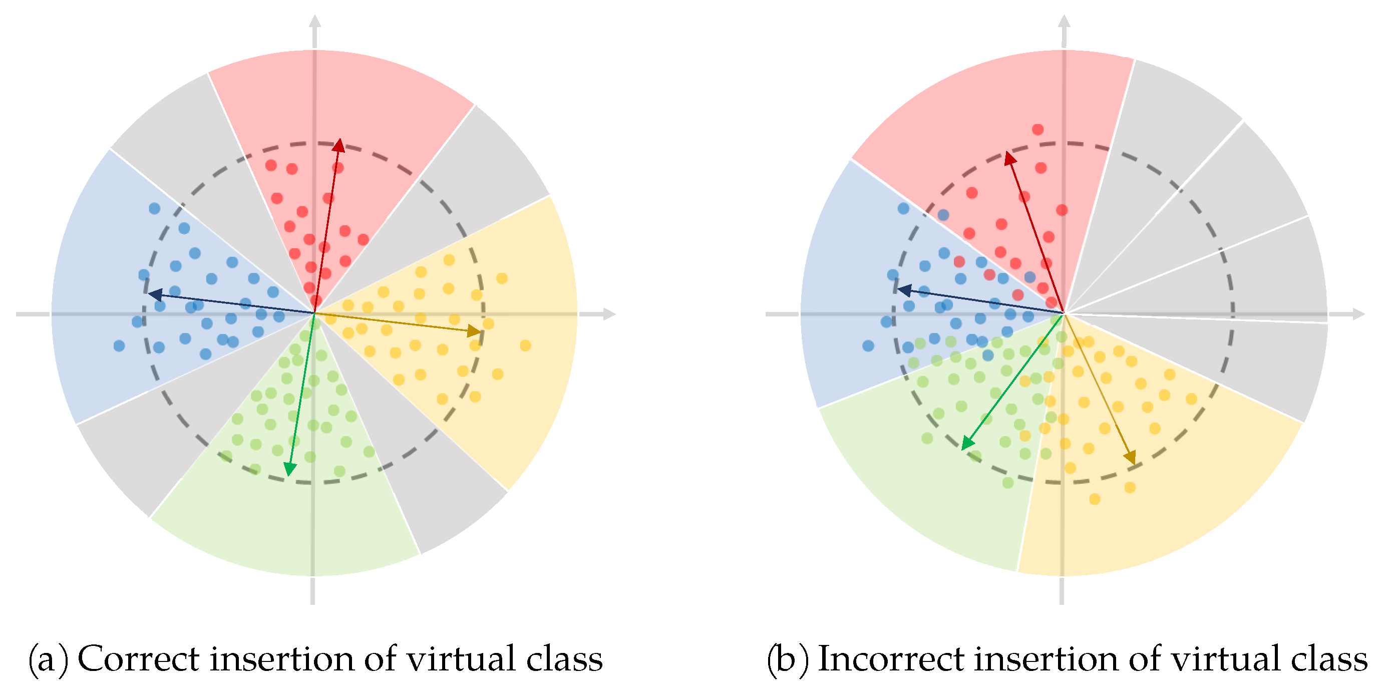
The virtual class is a paradox, which is an artificial class that does not exist in the real classification problem, opposed to real classes. That means there is no sample in the dataset belonging to the virtual class but it exists in the feature space. On the one hand, there is no sample so all samples belonging to the real classes will keep away from it. On the other hand, it exists in the feature space so it can pull apart the adjacent real classes. By inserting a virtual class to every two real classes, the intra-class feature space is compressed and the inter-class feature space is pulled apart, and the ReID problem of intra-class variation and inter-class similarity may be solved. This idea is shown in the Figure 10a, in which the gray areas indicate the inserted virtual classes.
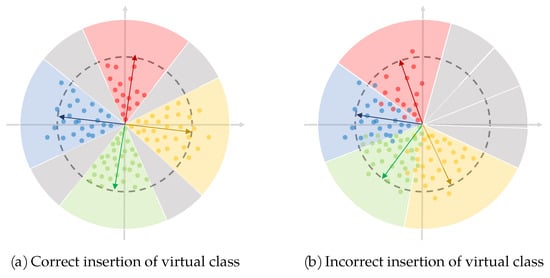
Figure 10.
Correct and incorrect insertion of virtual classes.
Introducing virtual class to vehicle ReID task is intuitively feasible, but the difficulty lies that how to insert the virtual class into two real classes accurately, for the FC layer of network is randomly initialized and it is difficult to track the change of the parameters during back propagation. If the virtual class is not inserted accurately, the opposite result is caused—further aggravating the problem of feature space confusion, as shown in Figure 10b.
To avoid incorrect insertion of virtual class, we take the work of Chen et al. [26] as reference and discard the method of Zheng et al. [27], creating a new loss function called Normalized Virtual Softmax Loss (NV-softmax Loss). The process is as follows.
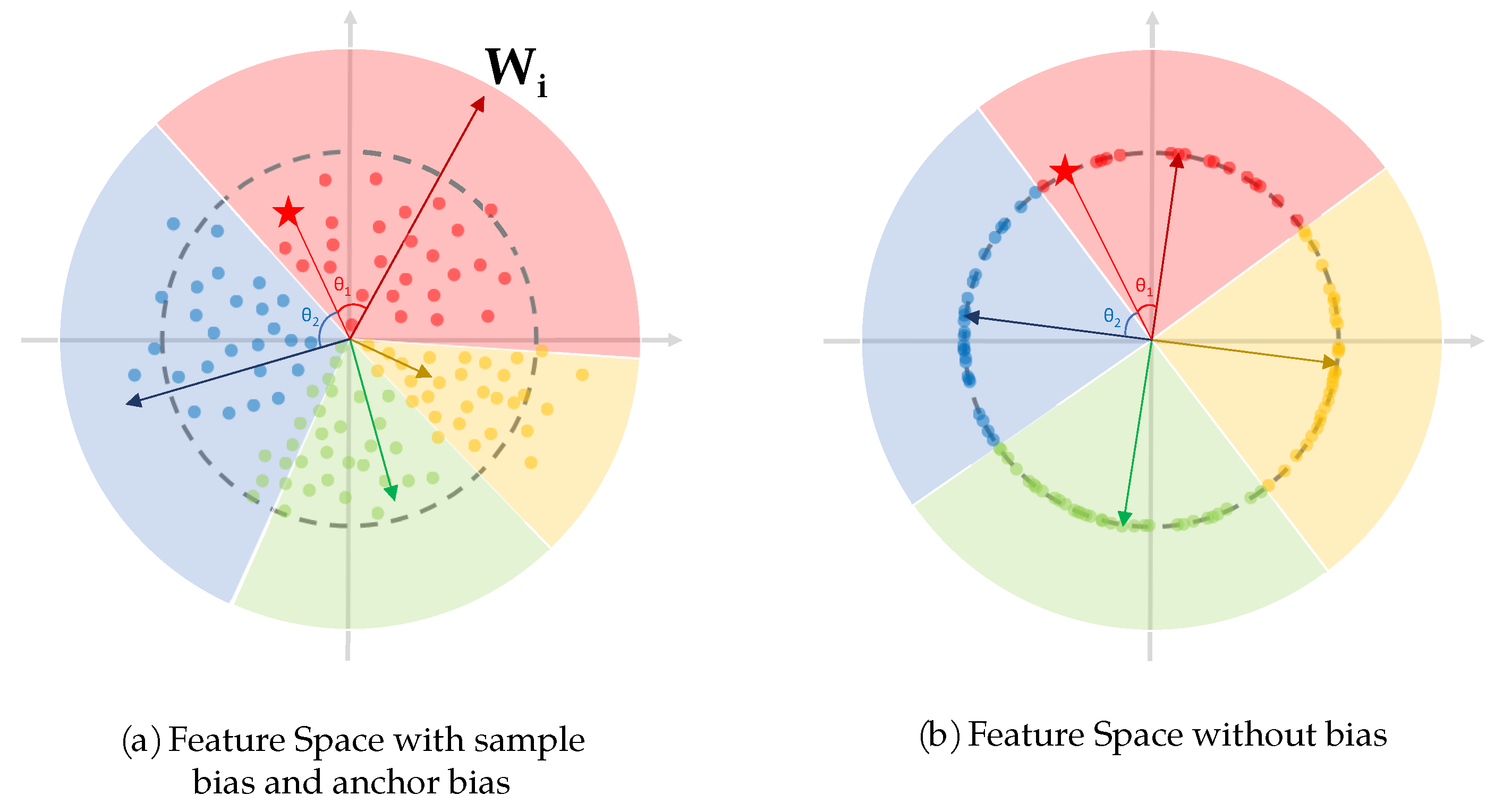
Firstly, the output of the feature extraction network X is normalized to (Equation (8)) to eliminate the sample bias that exists in original virtual softmax (Figure 11). From Equation (21), it is easy to see that affect the results of back propagation, which resulting in a sample-dependent bias and affects the performance of the network. Furthermore, this kind of bias just come from the network parameters and have nothing to do with the dataset, so it is endogenous bias and should be avoided as much as possible.
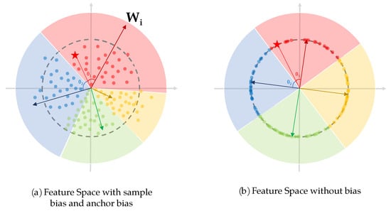
Figure 11.
The feature space with and without bias.
Secondly, in the FC layer, the row vectors of the weight matrix is normalized to (Equation (9)) to eliminate the anchor bias which exists in the original virtual softmax (Figure 11). It is also endogenous bias. In Equation (2), the class with larger occupies larger region in the feature space (boundary condition is , so when , , as shown in Figure 11). This may not affect the performance of the network in an ordinary classification task, but in the vehicle ReID task with a large number of classes, the original virtual softmax may constrain some classes’ feature space too small, increasing the possibility of misclassification. In order to make the feature spaces of all classes in the same size, we do a row normalization of W from to .
Thirdly, we construct the class anchor of the virtual class using the sample itself (Equation (10)). In this way, the virtual class is successfully inserted between two real classes, while no sample’s ground truth belongs to the virtual class. Here the sample vector has been normalized in the first step when eliminating the sample bias, so we can just insert into directly. The placement of the insertion is of no difference, and for convenience it is inserted into the last row, which constitutes (Equation (11)). is multiplied with to obtain , and is normalized by softmax function to get . Referring to Equations (3) and (4), the process above can be described as Equation (12) and Equation (13), respectively. Finally a new loss is produced (Equation (14)). In the next training round, the virtual class of the previous round is discarded and new training sample becomes the anchor of the new virtual class, thus preventing the situation of incorrect insertion in which two virtual class are neighboring. The process is illustrated in Figure 9b, and a more compact feature space is created in which .
L is the sum of each in a training batch, so for convenience we focus only on . The loss back propagates, changing the network parameters, acts on the feature extraction network and FC layer as shown in Equation (15), Equation (16) and Equation (17), respectively. Here, it needs to be emphasized that (1) , and are all unit vector, so some of the calculation is easy such as in Equation (16); (2) the derivative of the modulus of a vector with respect to itself is equal to the transpose of the unit vector corresponding to this vector, which means in Equation (16).
Comparing to the original virtual softmax proposed by [26], the operation of normalization not only eliminates the bias coming from the network, but also simplifies the calculation of back propagation above. However, we don’t do the simplification because we hope our proof to be more generalized as a reference for original virtual softmax loss. Furthermore, normalized virtual softmax loss has a more specific geometric meaning than original virtual softmax loss, where the dot product of the feature vector and class anchor degenerates into the calculation of the angle between them, for .
4.2. Comparison between Softmax and NV-Softmax
Here we compare the effects of the back propagation in original softmax loss and normalized virtual softmax loss.
The image input enters the network and goes through feature extraction network containing many convolutional and pooling layers. It would be troublesome to derive back propagation in such a complex network structure. Therefore, we use a toy model containing only one linear network and one activation function to derive. Considering that convolutional layers is a superposition of linear layer, and operations of pooling and normalization do not generate gradients, this toy model is without loss of generality.
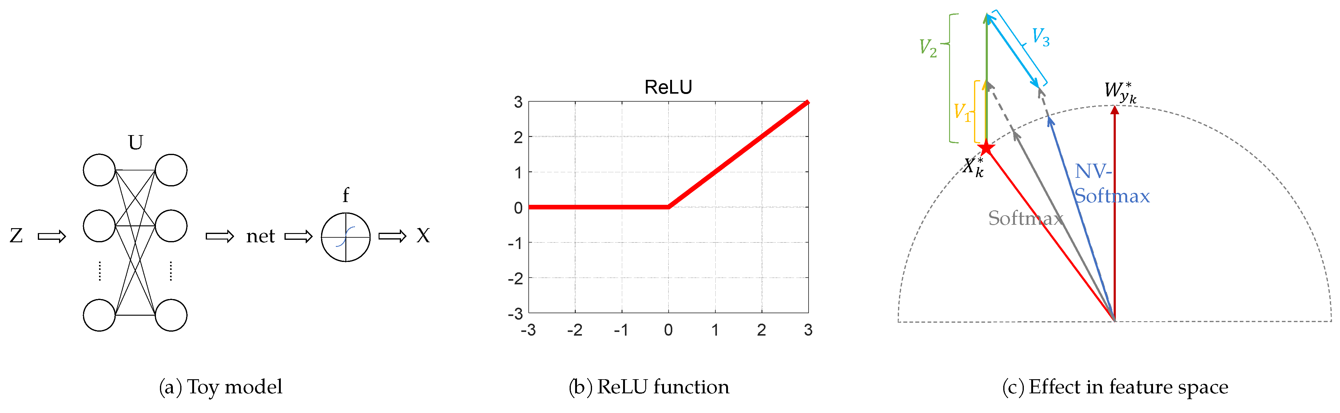
Suppose the input of the toy model is the fixed Z, the weight matrix of the linear network is U, the bias is 0, the output of the linear network is net, the activation function is f(·), the output of the activation function is X, and the learning rate is , shown in Figure 12a. The variables after one back propagation are , ,, respectively. We obtain:
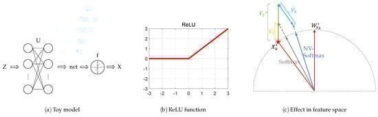
Figure 12.
(a) The toy model. (b) The ReLU function. (c) The comparison between softmax and NV-softmax.
The activation function in the feature extraction network Resnet in our model is the rectified linear unit (ReLU), and the ReLU function is a linear function with derivative equal to 1 in the activation interval (Figure 12b); thus,
where .
Because , and is the ground truth class anchor of , in a well trained network, >> , >> , >> , ∀. Furthermore, the exponential nature of e exacerbates the differences above. Hence, we can simplify the above two equations as follows, respectively:
Figure 12c shows the position of , , , , and in the feature space. is represented by a pentagram, and the gray dashed semicircle is the unit circle. The blue vector and the gray vector indicate the sample’s position trained by NV-softmax loss and original softmax loss, respectively. is parallel to and , and is parallel to . Here for convenience we hypothesize , so > . It is easy to see that comparing with the one trained by original softmax loss, the network trained by normalized virtual softmax loss can bring the sample closer to its class anchor, leading to a more compressed feature space. Since, in our model, every time, the samples enter into the FC layer they will be normalized, so the final location of the sample trained by different softmax loss are on the unit circle.
4.3. Our Model
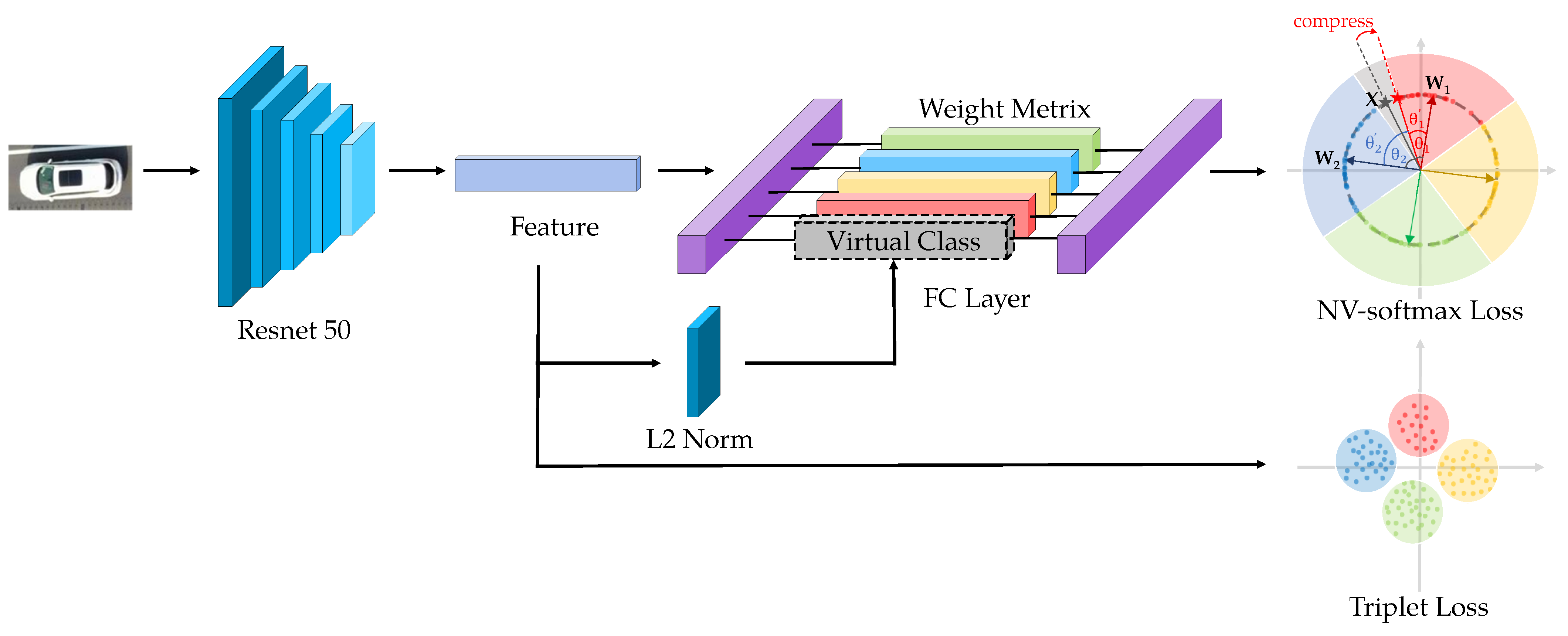
We propose our model as shown in Figure 13.

Figure 13.
The pipeline of our model.
Resnet-50 [13] is widely used in Vehicle ReID task as a backbone because of its excellent performance. We use it as the feature extraction network but we modify the last FC layer to make full use of our proposed normalized virtual softmax loss.
Normalized virtual softmax loss is one of the classification losses that divide the feature space into several subspaces belonging to different classes, which intersect at a centroid (when the bias of FC layer is set to 0, this centroid is the origin of the coordinate system). The classification loss has two characteristics. First, the cosine distance with the centroid of feature space as the vertex is more appropriate than the Euclidean distance, leaving alone that in normalized virtual softmax loss all of the samples and the class anchors are on the unit circle. Second, classification loss pre-sets the goal of each class to converge by initializing the anchor, which is a global constraint.
In the ReID task, triplet loss is also used in addition to classification loss. The essence of triplet loss is to pull in the intra-class samples and push away the inter-class samples, which can solve the problem faced in vehicle ReID task [33]. In every training round, one sample is chosen as anchor, another sample in same class is chosen as positive sample while another sample in different class is chosen as negative sample. The loss is calculated in Equation (24), where is the distance between anchor and positive sample and is the distance between anchor and negative sample. Margin is a hyperparameter. Obviously, it is meaningless to use cosine distance in triplet loss, and Euclidean distance should be used instead. Furthermore, triplet loss only draws a number of positive and negative samples for training at a time, so it is a local constraint, and there is a possibility that the intra-class distance is larger than the inter-class distance due to the local constraint.
The classification loss provides a strong supervision for global constraint while triplet loss finely trains the samples group by group. The introduction of triplet loss enhances the ability of network to compress the intra-class space and pull apart the inter-class pace, which create synergy with normalized virtual softmax loss, so we combine them (Equation (25)) to solve the problem of intra-class difference and inter-class similarity widespread in vehicle ReID task. The value of NV-softmax loss always differs from that of triplet loss by one order of magnitude in the beginning of training. We want triplet loss to player a role as a more accurate supervisor after NV-softmax loss roughly converges, so we set to take advantage of the difference in magnitude.
Due to the inconsistent of the metric distance used by normalized virtual softmax loss and triplet loss, the convergence of different loss functions’ backpropagation may be contradictory (Figure 14). Samples trained by normalized virtual softmax is going to get closer to the class anchor along the unit circle while samples trained by triplet loss tend to get closer to other positive samples. To solve the problem we use the feature vectors before and after L2 normalization operation for the triplet loss and normalized feature loss, respectively. In other words, we use triplet loss with Euclidean distance to optimize the original feature distribution from Resnet-50, while normalize to to make full use of the sample unbiasedness and anchor unbiasedness in normalized virtual softmax loss with cosine distance.
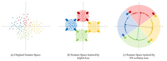
Figure 14.
The feature space trained by different loss functions.
5. Results
We evaluate our model on two UAV-based dataset—big dataset VRAI and small dataset VRAI_AIR. At the same time, to demonstrate the effectiveness of our model, we test it on the large dateset VehicleID and the small dataset VeRi based on the city surveillance system. In addition to comparing with baseline, we also compare with other softmax-based improvements, including angular softmax (A-softmax) [25] and virtual softmax (V-softmax) [26]. We use Rank-1, Rank-5, Rank-10 [34], and mean Average Precision (mAP) [35] as evaluation metrics.
In the experiments, we use Resnet-50 pre-trained on ImageNet as the feature extraction network. We set the mini-batch size to 64, with 16 IDs and 4 images per ID. All images are resized to 256 × 256 pixels. There are 120 training epochs. The learning rate is and decreased to at the 60th epoch. The margin of triplet loss is 0.3. We use Xavier Initialization [36] to initial all kinds of softmax to better suit the ReID task. All experiments are performed on four NVIDIA GeForce RTX 3090.
In the experiments on VRAI-AIR, we omit some of the evaluation metrics such as Rank-5 and Rank-10 because these metrics reach 100% due to the small size of the dataset. VehicleID dataset have three test sets called small, medium and large, respectively. To make results more reliable, we test the model on its hlmedium test set.
5.1. Ablation Experiments
We conduct ablation experiments on four dataset VRAI (Table 1), VRAI_AIR (Table 2), VehicleID (Table 3) and VeRi (Table 4). In the experiments, we train and test the model containing only softmax loss and NV-softmax loss, respectively. Then we add triplet loss to the above two models and perform the experiments separately.

Table 1.
Ablation experiments on VRAI.
Table 2.
Ablation experiments on VRAI-AIR.
Table 3.
Ablation experiments on VehicleID.
Table 4.
Ablation experiments on VeRi.
From the experients, we find that NV-softmax loss performs better than the original softmax loss, achieving 0.63%, 0.23%, 0.75% and 0.28% improvements on Rank-1 on these four dataset, respectively. The effect of triplet loss is obvious, which can enhance the discriminative ability of the model by 3.7%, 0.82%, 2.33% and 1.98% on Rank-1 on these four dataset, respectively. The co-training of NV-softmax loss and triplet loss create synergistic effects, achieves 76.70%, 98.95%, 76.85% and 92.79% on Rank-1 on these four dataset. The other metrics are also improved.
5.2. Comparison Experiments
We conduct comparison experiments on four dataset VRAI (Table 5), VRAI_AIR (Table 6), VehicleID (Table 7) and VeRi (Table 8). In the experiments, we compare our model with several other models for global feature and improved softmax. Baseline is original softmax loss with triplet loss. A-softmax [25] means angular softmax, which jointly use the angularly constrained classification loss and triplet loss. V-softmax [26] refers to original virtual softmax loss with triplet loss. Our model uses normalized virtual softmax loss and triplet loss.
Table 5.
Comparison experiments on VRAI.
Table 6.
Comparison experiments on VRAI-AIR.
Table 7.
Comparison experiments on VehicleID.
Table 8.
Comparison experiments on VeRi.
Experiments show that on most datasets our model achieves better performance compared to baseline and virtual softmax, achieving 76.70% of Rank-1 on the VRAI dataset, 98.95% on the VRAI-AIR dataset, and 92.79% on the VeRi dataset, which is the best performance among softmax improvements for global features. However, on the VehicleID dataset, we observe that the Rank-1 of our model is lower than that of A-softmax. In the other metrics such as Rank-5, Rank-10 and mAP, our method outperforms on all of the datasets.
5.3. Visualization Experiments
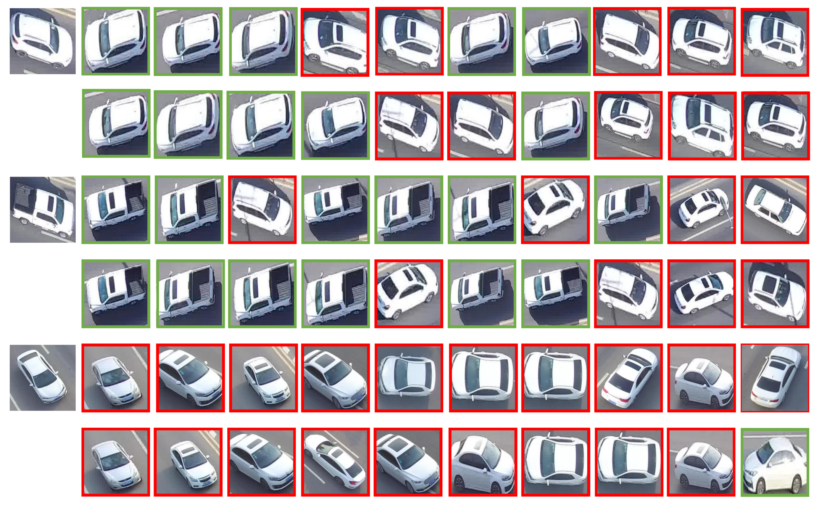
To visually demonstrate the advantage of our approach, here we give three examples of the model’s output in Figure 15. To each sample, the top 10 returned results of two methods are displayed in two line according to the similarities to the sample. The first line shows the results of the model trained by baseline (original softmax loss + triplet loss) and the second line shows the results of our model (normalized virtual softmax loss + triplet loss). Green boxes represent the the true positive results while the red boxes represent the false positive results.
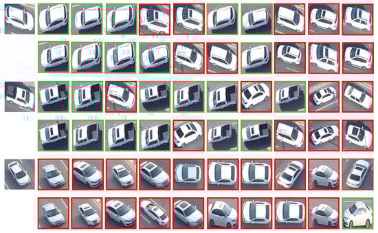
Figure 15.
Visualization results on VRAI dataset. For each query, the first line shows the results of baseline and the second line of our method. True positive results are in green boxes while false positive results in red.
In the first two examples, it is easy to see that in our method the position of true positive results in green boxes are more forward, because we increase similarities of intra-class samples and decreasing them of inter-class samples by normalized virtual softmax loss. That leads to improvements in all the metrics of Rank-1, Rank-5, Rank-10 and mAP. In some extreme cases, the third query for example, our model can at least promote the position of true positive results into top 10 list. Considering that in the practical application people often check the top 10 list manually, our method can provide a better reference value.
6. Discussion
In this section, we explain the results of the experiments, and discuss the practical applications of our research, as well as the future work.
Generally speaking, the experiments show the NV-softmax loss works and performs better than the original softmax loss and other softmax-based loss such as the A-softmax and V-softmax. Comparing with using classification loss alone, the joint use of triplet loss can improve the model’s performance. In practical application, the return list of our method is intuitively better.
Furthermore, we observe an interesting thing in the ablation experiments that the boosting effect of NV-softmax loss on Rank-5 and Rank-10 is greater than that on Rank-1 (Table 1, Table 2, Table 3 and Table 4). This shows that for some hard samples, our method can make the score of the corresponding class of the ground truth as high as possible even if cannot classify the hard samples accurately, thus improving the returned results in top 5 or top 10 list. This point is also proven in the visualization experiments. In the practical application of vehicle ReID, the ranking list of the top 10 returned by the network is often checked manually by people to improve the accuracy. Our method improves the Rank-10 in the experiments greatly, thus has an important significance in practical applications.
Although our approach achieves excellent performance on most datasets and metrics, we observe that the Rank-1 of our model is lower than that of A-softmax on VehicleID dataset (Table 7). In theory, A-softmax compresses the region of each class in the feature space to 1/m of the original by mathematical transformation, which is a global hard constraint and thus achieve good performance. However, the computational process of A-softmax includes the multiplicative angle formula, which greatly increases the computational complexity. Considering that the advantage of A-softmax is not significant, our model with negligible additional computational complexity has better application prospects.
Improving the accuracy of the ReID algorithm is critical to help security departments accurately query, locate and track the suspect vehicles, and there is no doubt that our method achieves this goal. We are going to publish our dataset to facilitate the study on UAV-based vehicle ReID. Furthermore, we have integrated our approach into the FastReID framework [30], which is a practical product-level library. In the near future, we will deploy the code to UAVs for practical use.
Despite the good performance comparing with the other modified softmax loss, we know there are still some improvements that can be made. Firstly, our dataset is relatively small. Considering that some of the material we shot has not been fully labeled, we will continue to update our self-built dataset in the future. Secondly, the normalized virtual softmax loss is achieved by dynamically inserting virtual classes into the FC layer, which does not affect the main structure of the network. In the future, we hope to try to use the normalized virtual softmax loss in more advanced feature extraction networks, such as multiple granularities network (MGN) [37], recurrent-neural-network-based hierarchical attention model (RNN-HA) [38] and region-aware model (RAM) [39].
7. Conclusions
In this paper, we present several problems faced in UAV-based vehicle ReID task, including the lack of datasets, the multiplicity of viewpoint, and the confusion of visual features. These problems can be solved by introducing new datasets and loss functions. Therefore, we create our own UAV-based vehicle ReID dataset and describe the process and its various properties. We expect our dataset to contribute to the research of vehicle ReID on UAV platform. In addition, we propose a novel loss function called normalized virtual softmax loss which is achieved by dynamically inserting virtual classes into the FC layer. We illustrate it in the feature space and proof its effectiveness by mathematical method. We jointly use normalized virtual softmax loss and triplet loss to train Resnet-50 to create Synergy. The experiments on four vehicle ReID datasets show that our method is better than the original softmax loss and the other modified softmax losses. We have applied our approach to the practical framework, and in the future we will continue to update the dataset and method.
Author Contributions
Conceptualization, W.Q., W.R. and L.Z.; methodology, W.Q.; software, W.Q., L.Z.; validation, W.Q.; formal analysis, W.Q., W.R. and L.Z.; investigation, W.Q., W.R. and L.Z.; resources, W.Q., W.R. and L.Z.; data curation, W.Q., W.R. and L.Z.; writing—original draft preparation, W.Q.; writing—review and editing, W.Q., W.R. and L.Z.; visualization, W.Q.; supervision, W.R., L.Z.; project administration, W.R., L.Z. All authors have read and agreed to the published version of the manuscript.
Funding
This research received no external funding.
Institutional Review Board Statement
Not applicable.
Informed Consent Statement
Not applicable.
Data Availability Statement
VRAI-AIR: Please connect with the author Wenzuo Qiao by qiaowenzuo19@mails.ucas.ac.cn. VRAI: https://github.com/JiaoBL1234/VRAI-Dataset. VehicleID: https://www.pkuml.org/resources/pku-vehicleid.html. VeRi: https://vehiclereid.github.io/VeRi/.
Acknowledgments
Thanks to the providers of the three datasets: VRAI, VehicleID and VeRi.
Conflicts of Interest
The authors declare no conflict of interest.
Abbreviations
The following abbreviations are used in this manuscript:
| MDPI | Multidisciplinary Digital Publishing Institute |
| DOAJ | Directory of open access journals |
| NV-softmax | Normalized virtual softmax |
| V-softmax | Virtual softmax |
| A-softmax | angular softmax |
References
- Zheng, Y.; Capra, L.; Wolfson, O.; Yang, H. Urban computing: Concepts, methodologies, and applications. ACM Trans. Intell. Syst. Technol. 2014, 5, 1–55. [Google Scholar] [CrossRef]
- Sobel, D.; Jędrasiak, K.; Nawrat, A. Simulation of Multi-Camera Indoor and Outdoor 3D Scanner. J. Eng. Sci. Res. 2018, 2, 33–41. [Google Scholar] [CrossRef]
- Prabhakaran, A.; Sharma, R. Autonomous Intelligent UAV System for Criminal Pursuit—A Proof of Concept. Indian Police J. 2021, 68, 1–20. [Google Scholar]
- Wang, P.; Jiao, B.; Yang, L.; Yang, Y.; Zhang, S.; Wei, W.; Zhang, Y. Vehicle re-identification in aerial imagery: Dataset and approach. In Proceedings of the IEEE/CVF International Conference on Computer Vision, Seoul, Korea, 27–28 October 2019; pp. 460–469. [Google Scholar]
- Lin, T.Y.; Maire, M.; Belongie, S.; Hays, J.; Perona, P.; Ramanan, D.; Dollár, P.; Zitnick, C.L. Microsoft coco: Common objects in context. In Proceedings of the European Conference on Computer Vision, Munich, Germany, 8–14 September 2014; pp. 740–755. [Google Scholar]
- Ye, M.; Shen, J.; Lin, G.; Xiang, T.; Shao, L.; Hoi, S.C. Deep learning for person re-identification: A survey and outlook. IEEE Trans. Pattern Anal. Mach. Intell. 2021, 1–20. [Google Scholar] [CrossRef] [PubMed]
- Teng, S.; Liu, X.; Zhang, S.; Huang, Q. Scan: Spatial and channel attention network for vehicle re-identification. In Proceedings of the 19th Pacific-Rim Conference on Multimedia, Hefei, China, 21–22 September 2018; pp. 350–361. [Google Scholar]
- Chu, R.; Sun, Y.; Li, Y.; Liu, Z.; Zhang, C.; Wei, Y. Vehicle re-identification with viewpoint-aware metric learning. In Proceedings of the IEEE/CVF International Conference on Computer Vision, Seoul, Korea, 27 October–2 November 2019; pp. 8282–8291. [Google Scholar]
- Liu, X.; Liu, W.; Mei, T.; Ma, H. A deep learning-based approach to progressive vehicle re-identification for urban surveillance. In Proceedings of the 14th European Conference on Computer Vision, Amsterdam, The Netherlands, 11–14 October 2016; pp. 869–884. [Google Scholar]
- Liu, H.; Tian, Y.; Yang, Y.; Pang, L.; Huang, T. Deep relative distance learning: Tell the difference between similar vehicles. In Proceedings of the IEEE Conference on Computer Vision and Pattern Recognition, Las Vegas, NV, USA, 27–30 June 2016; pp. 2167–2175. [Google Scholar]
- Xia, G.S.; Bai, X.; Ding, J.; Zhu, Z.; Belongie, S.; Luo, J.; Datcu, M.; Pelillo, M.; Zhang, L. DOTA: A large-scale dataset for object detection in aerial images. In Proceedings of the IEEE Conference on Computer Vision and Pattern Recognition, Salt Lake City, UT, USA, 18–22 June 2018; pp. 3974–3983. [Google Scholar]
- Zhu, P.; Wen, L.; Du, D.; Bian, X.; Fan, H.; Hu, Q.; Ling, H. Detection and Tracking Meet Drones Challenge. arXiv 2020, arXiv:2001.06303. [Google Scholar] [CrossRef] [PubMed]
- He, K.; Zhang, X.; Ren, S.; Sun, J. Deep residual learning for image recognition. In Proceedings of the IEEE Conference on Computer Vision and Pattern Recognition, Las Vegas, NV, USA, 27–30 June 2016; pp. 770–778. [Google Scholar]
- Zeiler, M.D.; Fergus, R. Visualizing and understanding convolutional networks. In Proceedings of the 13th European Conference on Computer Vision, Zurich, Switzerland, 6–12 September 2014; pp. 818–833. [Google Scholar]
- Deng, J.; Dong, W.; Socher, R.; Li, L.J.; Li, K.; Fei-Fei, L. Imagenet: A large-scale hierarchical image database. In Proceedings of the 2009 IEEE Conference on Computer Vision and Pattern Recognition, Miami, FL, USA, 20–25 June 2009; pp. 248–255. [Google Scholar]
- Dosovitskiy, A.; Beyer, L.; Kolesnikov, A.; Weissenborn, D.; Zhai, X.; Unterthiner, T.; Dehghani, M.; Minderer, M.; Heigold, G.; Gelly, S.; et al. An Image is Worth 16×16 Words: Transformers for Image Recognition at Scale. arXiv 2020, arXiv:2010.11929. [Google Scholar]
- He, S.; Luo, H.; Wang, P.; Wang, F.; Li, H.; Jiang, W. Transreid: Transformer-based object re-identification. In Proceedings of the IEEE/CVF International Conference on Computer Vision, Montreal, BC, Canada, 11–17 October 2021; pp. 15013–15022. [Google Scholar]
- Boltzmann, L. Studien uber das Gleichgewicht der lebenden Kraft. Wissenschafiliche Abh. 1868, 1, 49–96. [Google Scholar]
- Gibbs, J.W. Elementary Principles in Statistical Mechanics: Developed with Especial Reference to the Rational Foundations of Thermodynamics; C. Scribner’s Sons: New York, NY, USA, 1902. [Google Scholar]
- Bridle, J.S. Probabilistic interpretation of feedforward classification network outputs, with relationships to statistical pattern recognition. In Neurocomputing; Springer: Berlin/Heidelberg, Germany, 1990; pp. 227–236. [Google Scholar]
- Lu, C. Shannon equations reform and applications. BUSEFAL 1990, 44, 45–52. [Google Scholar]
- Rubinstein, R.Y. Optimization of computer simulation models with rare events. Eur. J. Oper. Res. 1997, 99, 89–112. [Google Scholar] [CrossRef]
- Zheng, L.; Zhang, H.; Sun, S.; Chandraker, M.; Yang, Y.; Tian, Q. Person re-identification in the wild. In Proceedings of the IEEE Conference on Computer Vision and Pattern Recognition, Honolulu, HI, USA, 21–26 July 2017; pp. 1367–1376. [Google Scholar]
- Liu, W.; Wen, Y.; Yu, Z.; Yang, M. Large-margin softmax loss for convolutional neural networks. arXiv 2016, arXiv:1612.02295. [Google Scholar]
- Liu, W.; Wen, Y.; Yu, Z.; Li, M.; Raj, B.; Song, L. Sphereface: Deep hypersphere embedding for face recognition. In Proceedings of the IEEE Conference on Computer Vision and Pattern Recognition, Honolulu, HI, USA, 21–26 July 2017; pp. 212–220. [Google Scholar]
- Chen, B.; Deng, W.; Shen, H. Virtual class enhanced discriminative embedding learning. Adv. Neural Inf. Process. Syst. 2018, 31. [Google Scholar]
- Zheng, Z.; Ruan, T.; Wei, Y.; Yang, Y.; Mei, T. VehicleNet: Learning robust visual representation for vehicle re-identification. IEEE Trans. Multimed. 2020, 23, 2683–2693. [Google Scholar] [CrossRef]
- Hermans, A.; Beyer, L.; Leibe, B. In defense of the triplet loss for person re-identification. arXiv 2017, arXiv:1703.07737. [Google Scholar]
- Wang, C.; Zhang, Q.; Huang, C.; Liu, W.; Wang, X. Mancs: A multi-task attentional network with curriculum sampling for person re-identification. In Proceedings of the European Conference on Computer Vision (ECCV), Munich, Germany, 8–14 September 2018; pp. 365–381. [Google Scholar]
- Luo, H.; Gu, Y.; Liao, X.; Lai, S.; Jiang, W. Bag of tricks and a strong baseline for deep person re-identification. In Proceedings of the IEEE/CVF Conference on Computer Vision and Pattern Recognition Workshops, Long Beach, CA, USA, 16–20 June 2019; pp. 4321–4329. [Google Scholar]
- Zhong, Z.; Zheng, L.; Cao, D.; Li, S. Re-ranking person re-identification with k-reciprocal encoding. In Proceedings of the IEEE Conference on Computer Vision and Pattern Recognition, Honolulu, HI, USA, 21–26 July 2017; pp. 1318–1327. [Google Scholar]
- Russell, B.C.; Torralba, A.; Murphy, K.P.; Freeman, W.T. LabelMe: A database and web-based tool for image annotation. Int. J. Comput. Vis. 2008, 77, 157–173. [Google Scholar] [CrossRef]
- Song, J.; Yang, Y.; Song, Y.Z.; Xiang, T.; Hospedales, T.M. Generalizable person re-identification by domain-invariant mapping network. In Proceedings of the IEEE/CVF conference on Computer Vision and Pattern Recognition, Long Beach, CA, USA, 16–20 June 2019; pp. 719–728. [Google Scholar]
- Wang, X.; Doretto, G.; Sebastian, T.; Rittscher, J.; Tu, P. Shape and appearance context modeling. In Proceedings of the 2007 IEEE 11th International Conference on Computer Vision, Rio de Janeiro, Brazil, 14–20 October 2007; pp. 1–8. [Google Scholar]
- Zheng, L.; Shen, L.; Tian, L.; Wang, S.; Wang, J.; Tian, Q. Scalable person re-identification: A benchmark. In Proceedings of the IEEE International Conference on Computer Vision, Santiago, Chile, 7–13 December 2015; pp. 1116–1124. [Google Scholar]
- Glorot, X.; Bengio, Y. Understanding the difficulty of training deep feedforward neural networks. In Proceedings of the Thirteenth International Conference on Artificial Intelligence and Statistics. JMLR Workshop and Conference Proceedings, Sardinia, Italy, 13–15 May 2010; pp. 249–256. [Google Scholar]
- Wang, G.; Yuan, Y.; Chen, X.; Li, J.; Zhou, X. Learning discriminative features with multiple granularities for person re-identification. In Proceedings of the 26th ACM International Conference on Multimedia, Seoul, Korea, 22–26 October 2018; pp. 274–282. [Google Scholar]
- Wei, X.S.; Zhang, C.L.; Liu, L.; Shen, C.; Wu, J. Coarse-to-fine: A RNN-based hierarchical attention model for vehicle re-identification. In Proceedings of the 14th Asian Conference on Computer Vision, Perth, Australia, 2–6 December 2018; pp. 575–591. [Google Scholar]
- Liu, X.; Zhang, S.; Huang, Q.; Gao, W. Ram: A region-aware deep model for vehicle re-identification. In Proceedings of the 2018 IEEE International Conference on Multimedia and Expo (ICME), San Diego, CA, USA, 23–27 July 2018; pp. 1–6. [Google Scholar]


Publisher’s Note: MDPI stays neutral with regard to jurisdictional claims in published maps and institutional affiliations. |
© 2022 by the authors. Licensee MDPI, Basel, Switzerland. This article is an open access article distributed under the terms and conditions of the Creative Commons Attribution (CC BY) license (https://creativecommons.org/licenses/by/4.0/).