
Aerodynamic Drag Reduction on Speed Skating Helmet by Surface Structures

Abstract
:1. Introduction
2. Numerical Approach
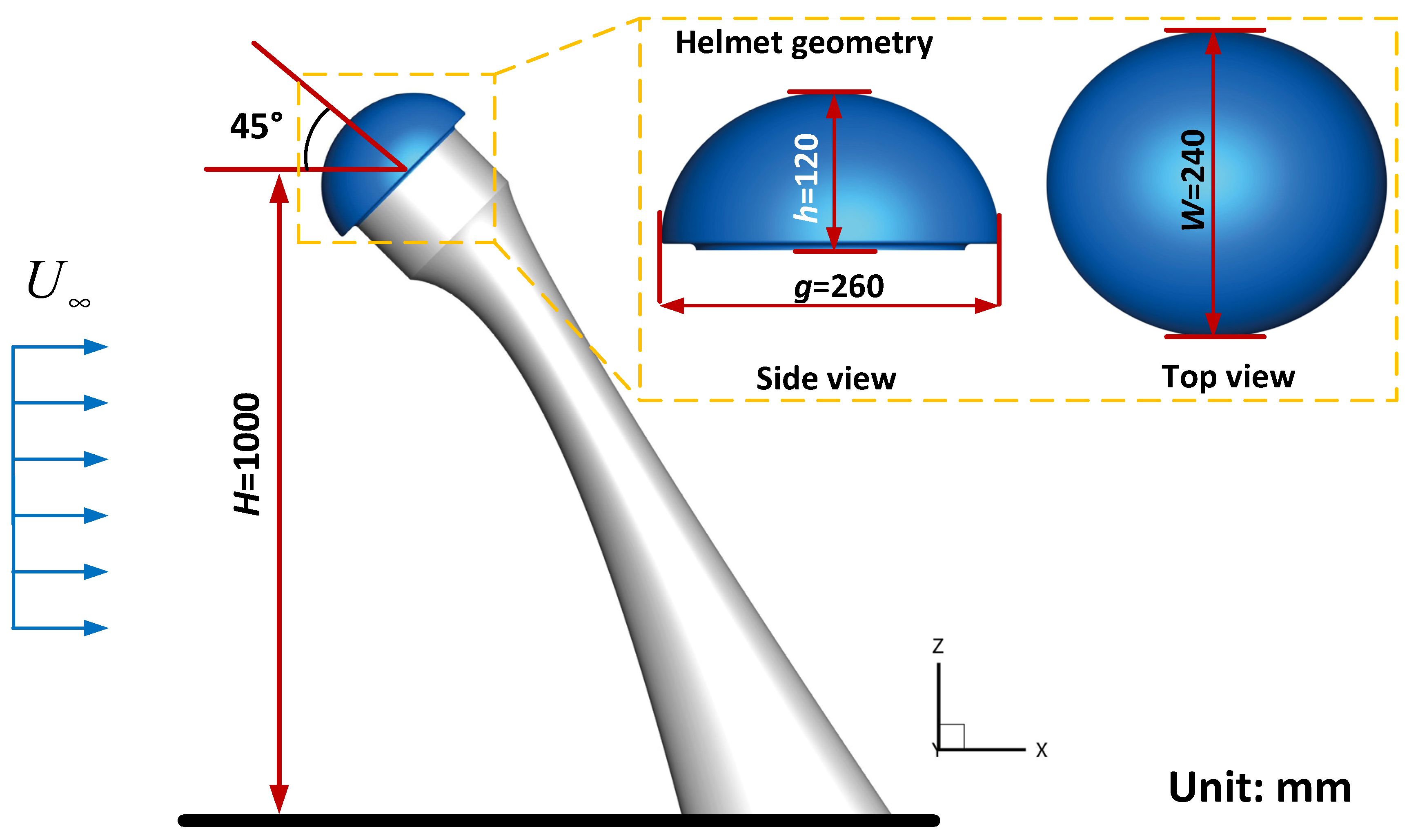
2.1. Computational Conditions and Helmet Models
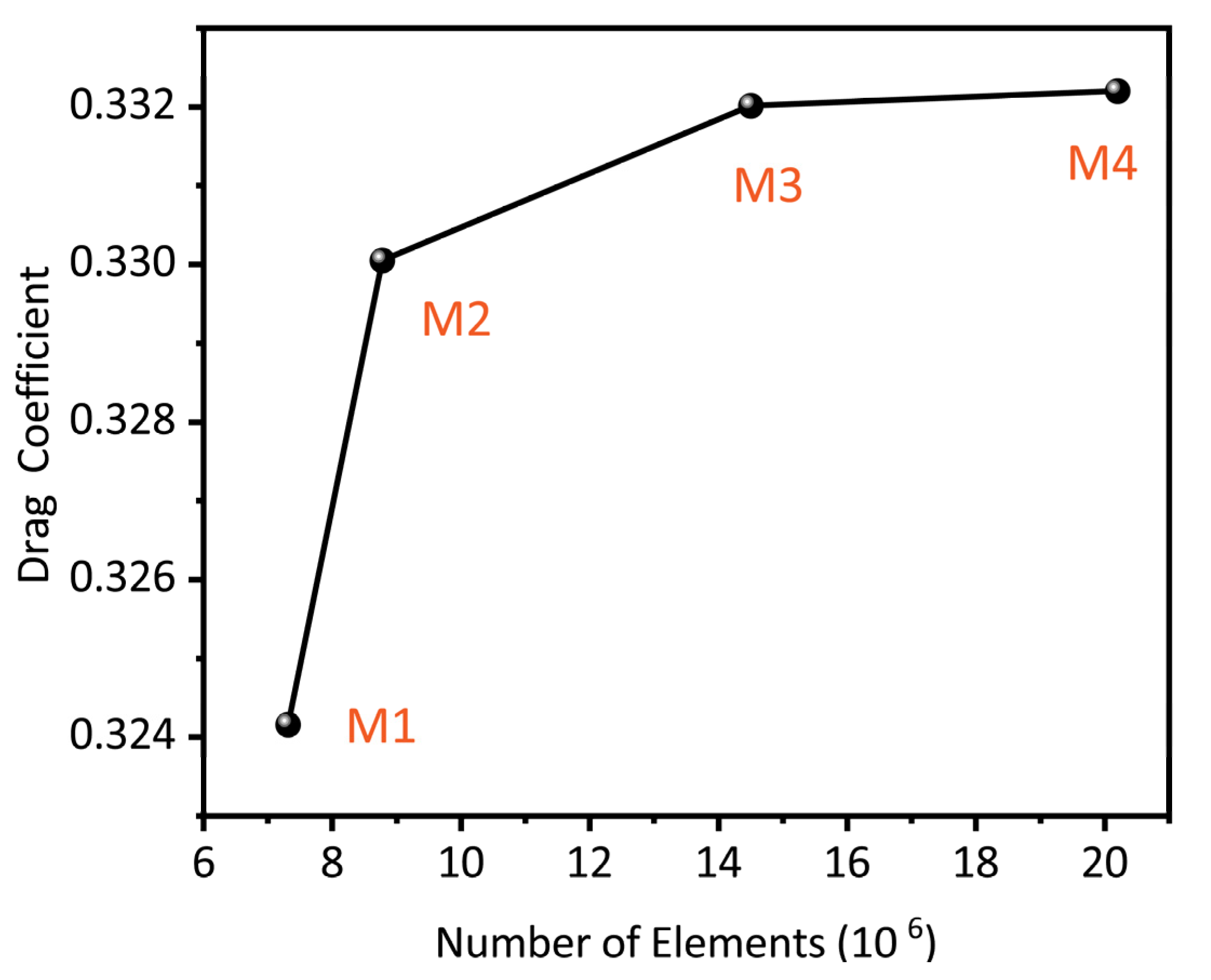
2.2. Slover Conditions and Mesh Convergence Research
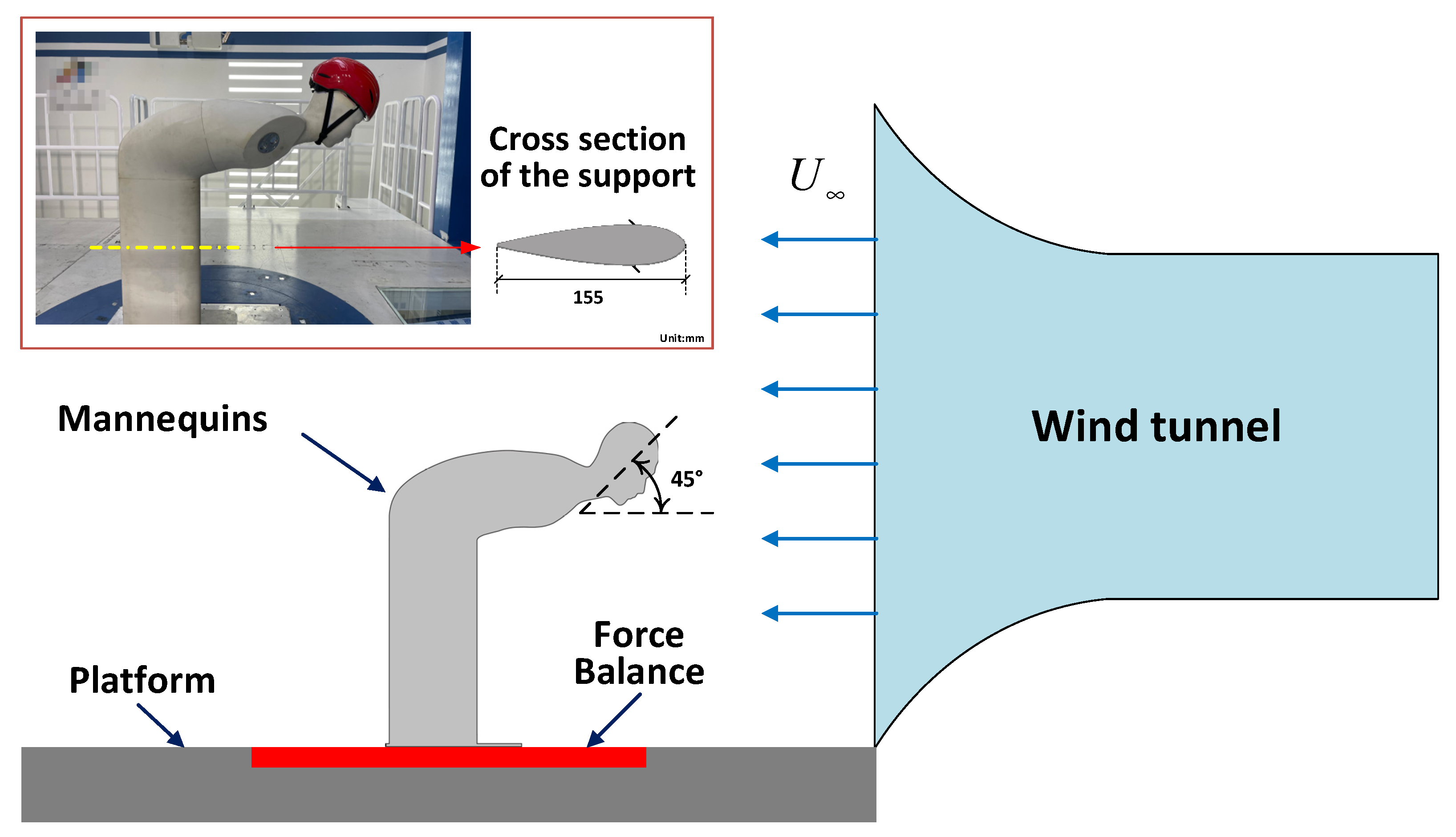
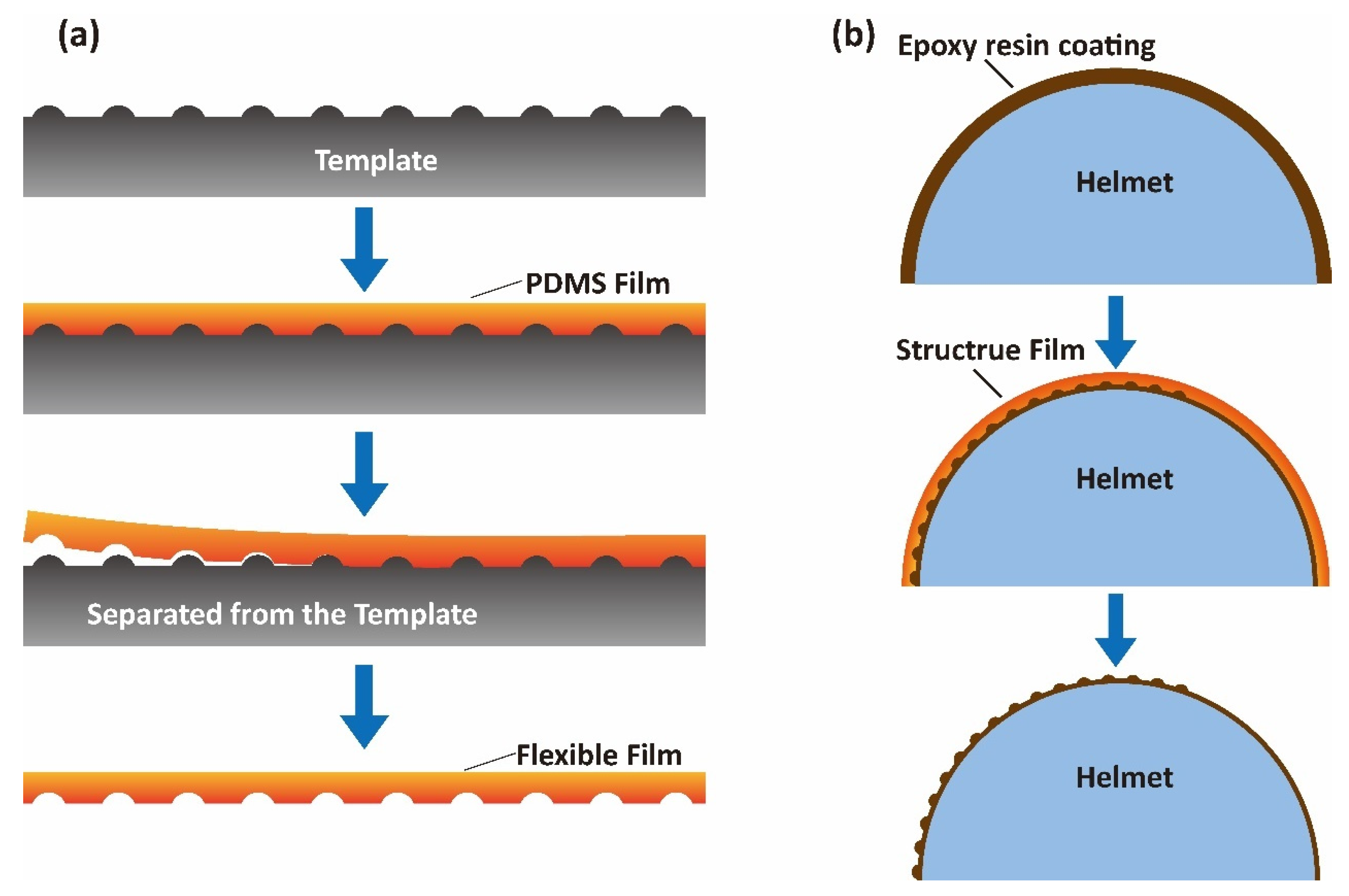
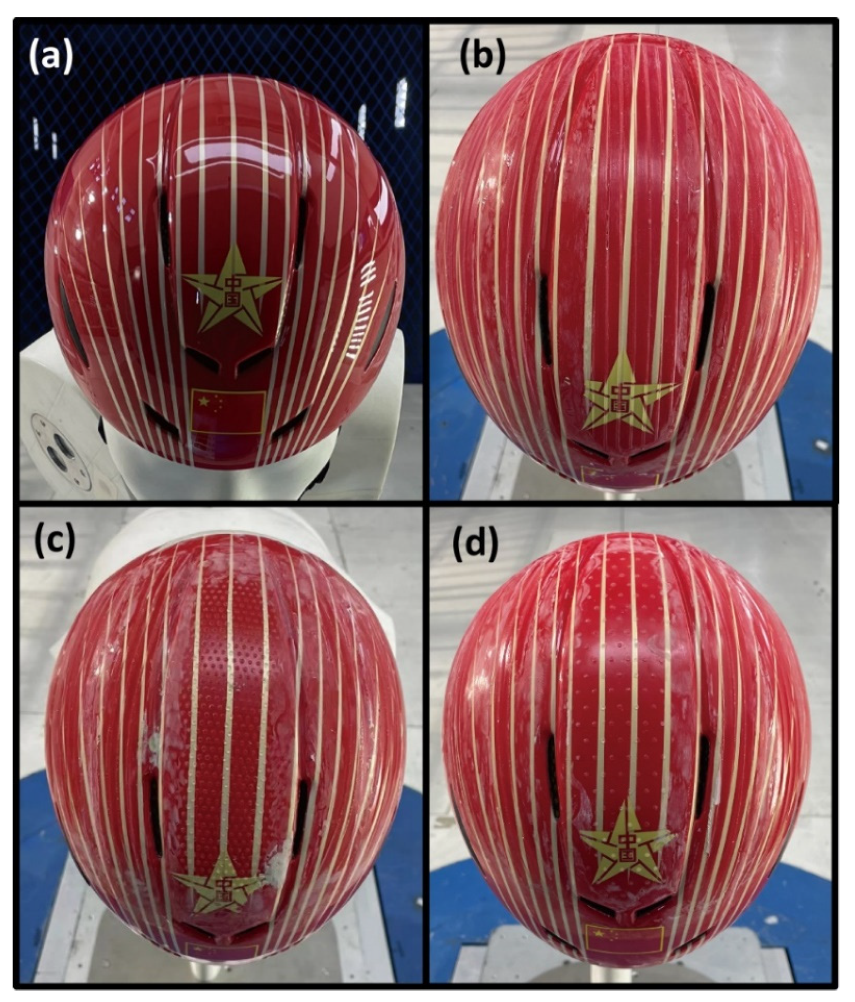
3. Experiment Method and Fabrication Process
4. Results and Discussion
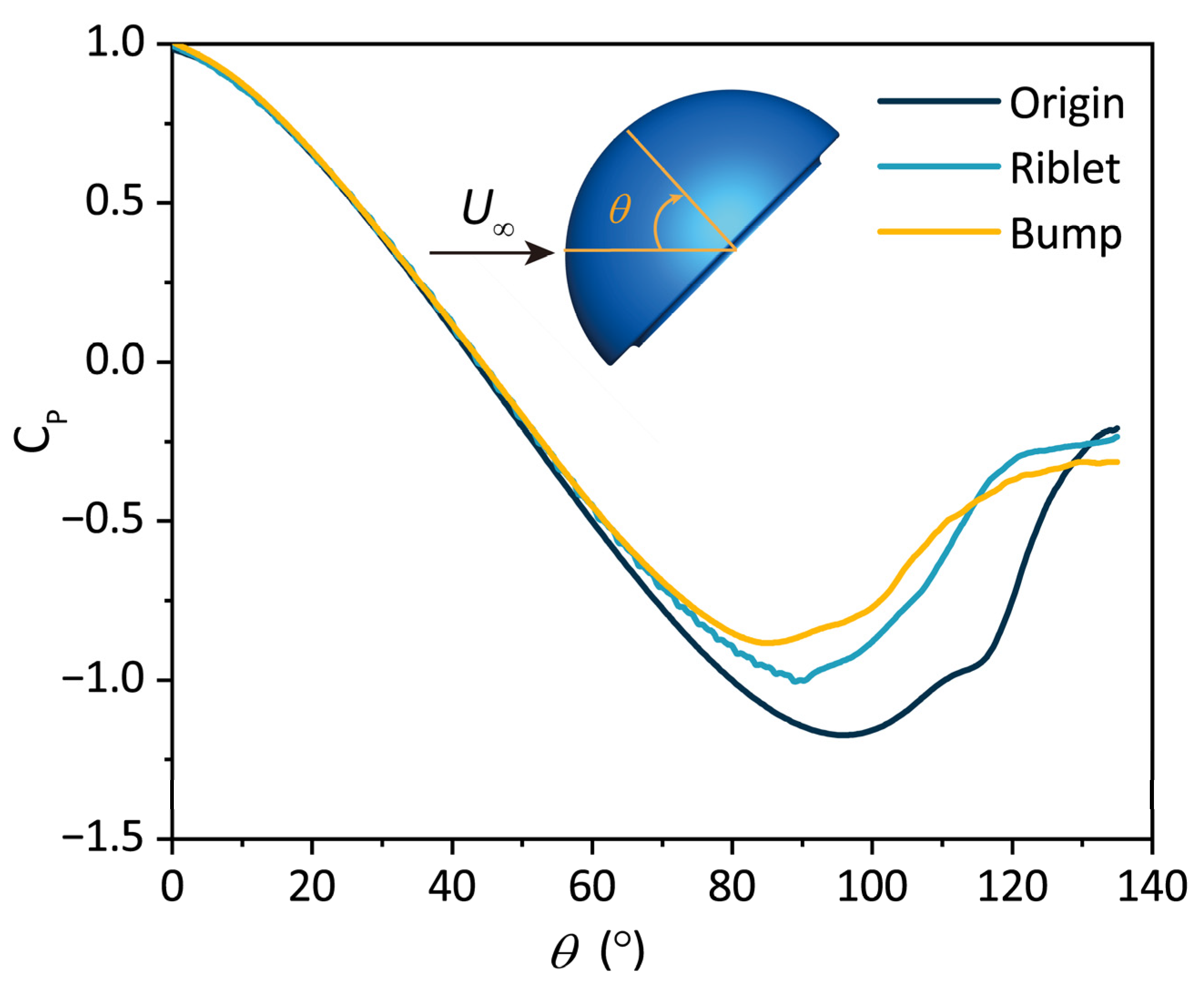
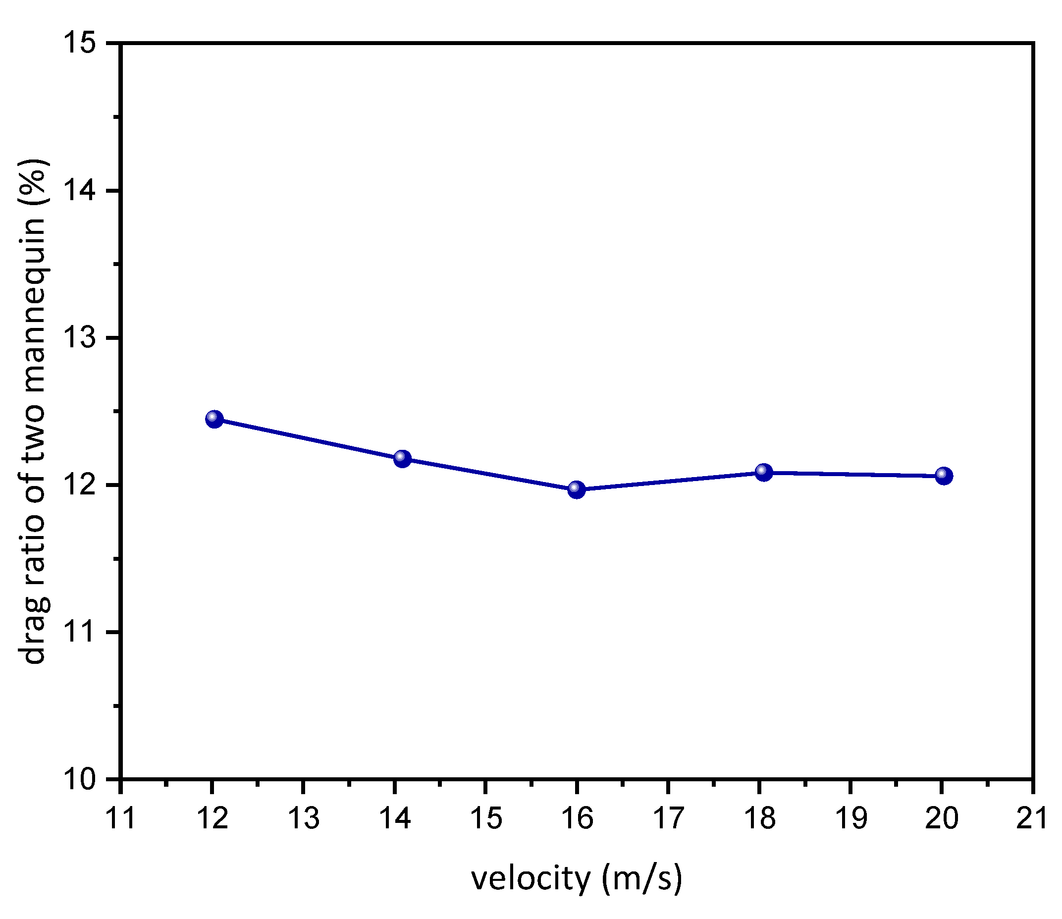
4.1. CFD and Experiment Results
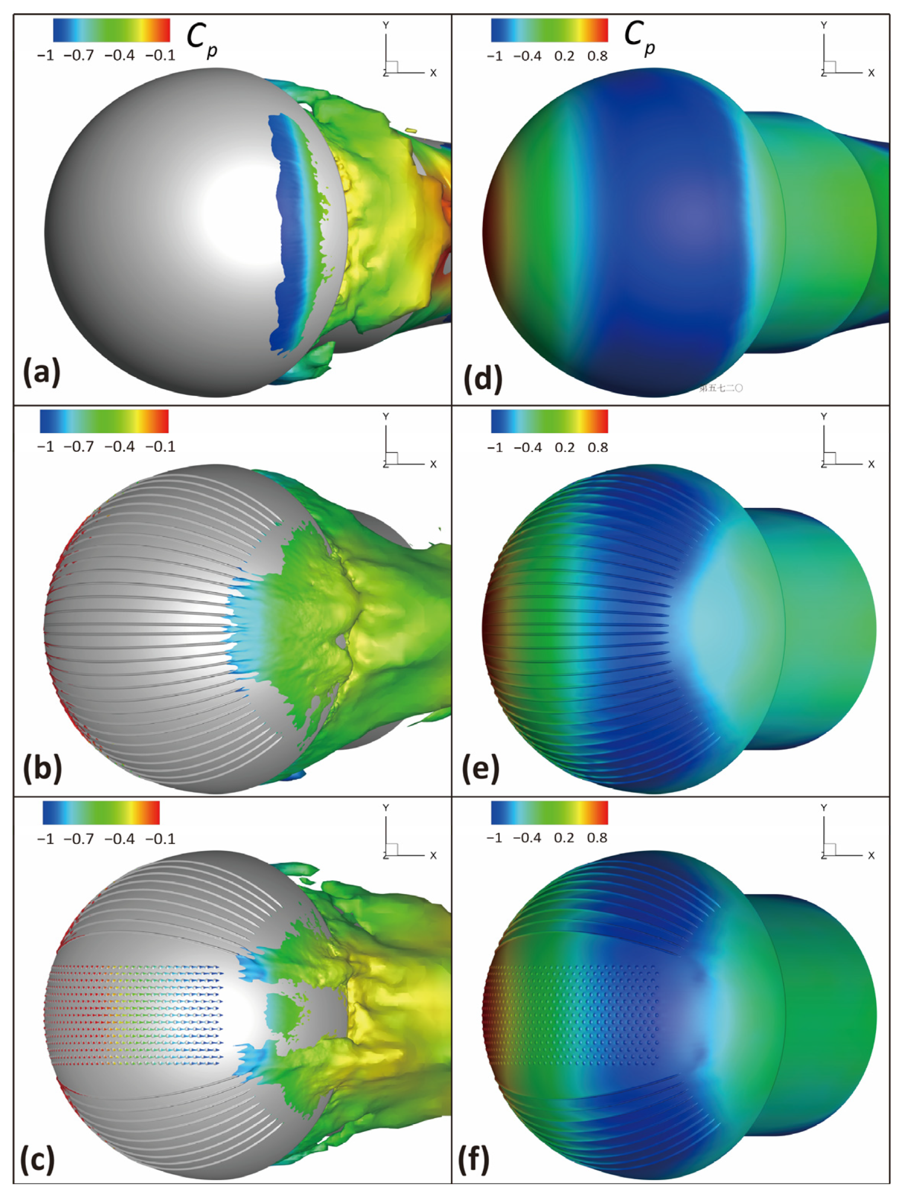
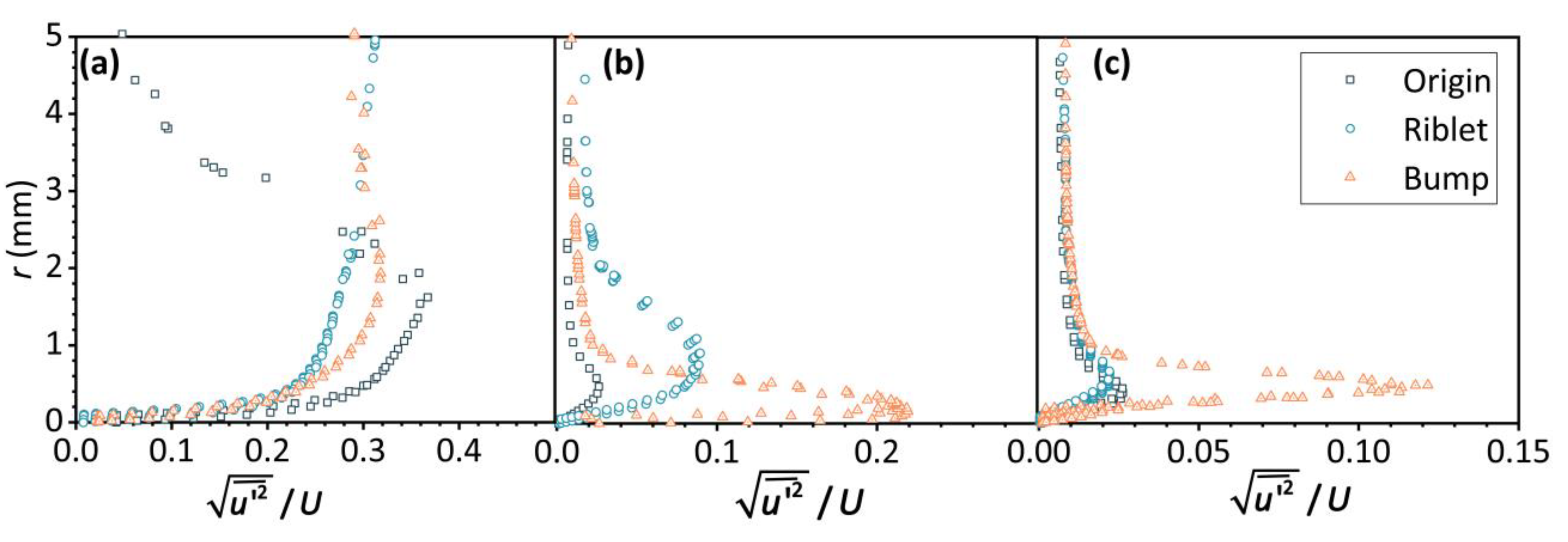
4.2. Fluid Field Profile
5. Conclusions
Author Contributions
Funding
Institutional Review Board Statement
Informed Consent Statement
Data Availability Statement
Acknowledgments
Conflicts of Interest
References
- Brownlie, L.; Ostafichuk, P.; Tews, E.; Muller, H.; Briggs, E.; Franks, K. The wind-averaged aerodynamic drag of competitive time trial cycling helmets. Procedia Eng. 2010, 2, 2419–2424. [Google Scholar] [CrossRef] [Green Version]
- Kimura, T.; Tsutahara, M. Fluid dynamic effects of grooves on circular cylinder surface. AIAA J. 1991, 29, 2062–2068. [Google Scholar] [CrossRef]
- Alam, F.; Chowdhury, H.; Wei, H.Z.; Mustary, I.; Zimmer, G. Aerodynamics of Ribbed Bicycle Racing Helmets. Procedia Eng. 2014, 72, 691–696. [Google Scholar] [CrossRef] [Green Version]
- Underwood, L.; Jermy, M.; Eloi, P.; Cornillon, G. Helmet position, ventilation holes and drag in cycling. Sport. Eng. 2015, 18, 241–248. [Google Scholar] [CrossRef]
- Javadi, A. Aerodynamic Study of the Pedalling of a Cyclist with a Transitional Hybrid RANS–LES Turbulence model. Flow Turbul. Combust. 2021, 108, 717–738. [Google Scholar] [CrossRef]
- Blocken, B.; Malizia, F.; Van Druenen, T.; Gillmeier, S. Aerodynamic benefits for a cyclist by drafting behind a motorcycle. Sport. Eng. 2020, 23, 19. [Google Scholar] [CrossRef]
- Forte, P.; Marinho, D.A.; Morouço, P.; Pascoal-Faria, P.; Barbosa, T.M. Comparison by Computer Fluid Dynamics of the Drag Force Acting Upon two Helmets for Wheelchair Racers. In Proceedings of the International Conference on Numerical Analysis and Applied Mathematics (ICNAAM), Rhodes, Greece, 19–25 September 2016. [Google Scholar]
- Beaumont, F.; Taiar, R.; Polidori, G.; Trenchard, H.; Grappe, F. Aerodynamic study of time-trial helmets in cycling racing using CFD analysis. J. Biomech. 2018, 67, 1–8. [Google Scholar] [CrossRef]
- Pathan, K.A.; Khan, S.A.; Shaikh, N.A.; Pathan, A.A.; Khan, S.A. An investigation of boat-tail helmet to reduce drag. Adv. Aircr. Spacecr. Sci. 2021, 8, 239–250. [Google Scholar]
- Puelles Magán, G.; Terra, W.; Sciacchitano, A. Aerodynamics Analysis of Speed Skating Helmets: Investigation by CFD Simulations. Appl. Sci. 2021, 11, 3148. [Google Scholar] [CrossRef]
- Bechert, D.; Bruse, M.; Hage, W.; Meyer, R. Biological surfaces and their technological application—Laboratory and flight experiments on drag reduction and separation control. In Proceedings of the 28th Fluid Dynamics Conference, Snowmass Village, CO, USA, 29 June–2 July 1997. [Google Scholar]
- Walsh, M.; Lindemann, A. Optimization and application of riblets for turbulent drag reduction. In Proceedings of the 22nd Aerospace Sciences Meeting 1984, Reno, NV, USA, 9–12 January 1984. [Google Scholar]
- Bechert, D.W.; Bruse, M.; Hage, W.; Meyer, R. Fluid mechanics of biological surfaces and their technological application. Naturwissenschaften 2000, 87, 157–171. [Google Scholar] [CrossRef]
- Koeltzsch, K.; Dinkelacker, A.; Grundmann, R. Flow over convergent and divergent wall riblets. Exp. Fluids 2002, 33, 346–350. [Google Scholar] [CrossRef]
- Dean, B.; Bhushan, B. Shark-skin surfaces for fluid-drag reduction in turbulent flow: A review. Philos. Trans. R. Soc.-Math. Phys. Eng. Sci. 2010, 368, 5737. [Google Scholar] [CrossRef]
- Ko, N.W.M.; Leung, Y.; Chen, J.J.J. Flow past V-groove circular cylinders. AIAA J. 1987, 25, 806–811. [Google Scholar] [CrossRef]
- Leung, Y.; Ko, N.W.M.; Leung, D.Y. Near wall characteristics of flow over grooved circular cylinder. Exp. Fluids 1991, 10, 322–332. [Google Scholar] [CrossRef]
- Yamagishi, Y.; Oki, M. Effect of Groove Shape on Flow Characteristics around a Circular Cylinder with Grooves. J. Vis. 2004, 7, 209–216. [Google Scholar] [CrossRef]
- Quintavalla, S.J.; Angilella, A.; Smits, A. Drag reduction on grooved cylinders in the critical Reynolds number regime. Exp. Therm. Fluid Sci. 2013, 48, 15–18. [Google Scholar] [CrossRef]
- Frohlich, C. Aerodynamic drag crisis and its possible effect on the flight of baseballs. Am. J. Phys. 1984, 52, 325–334. [Google Scholar] [CrossRef]
- Shih, W.; Wang, C.; Coles, D.; Roshko, A. Experiments on flow past rough circular cylinders at large Reynolds numbers. J. Wind Eng. Ind. Aerodyn. 1993, 49, 351–368. [Google Scholar] [CrossRef]
- Zhou, B.; Wang, X.; Gho, W.M.; Tan, S.K. Force and flow characteristics of a circular cylinder with uniform surface roughness at subcritical Reynolds numbers. Appl. Ocean Res. 2015, 49, 20–26. [Google Scholar] [CrossRef]
- Butt, U.; Jehring, L.; Egbers, C. Mechanism of drag reduction for circular cylinders with patterned surface. Int. J. Heat Fluid Flow 2014, 45, 128–134. [Google Scholar] [CrossRef]
- Choi, J.; Jeon, W.-P.; Choi, H. Mechanism of drag reduction by dimples on a sphere. Phys. Fluids 2006, 18, 041702. [Google Scholar] [CrossRef]
- Aoki, K.; Muto, K.; Okanaga, H. Mechanism of Drag Reduction by Dimple Structures on a Sphere. J. Fluid Sci. Technol. 2012, 7, 1–10. [Google Scholar] [CrossRef]


| Mesh | Elements | |
|---|---|---|
| M1 | 7,316,086 | 0.32416 |
| M2 | 8,779,304 | 0.33005 |
| M3 | 14,505,131 | 0.33202 |
| M4 | 20,200,985 | 0.3322 |
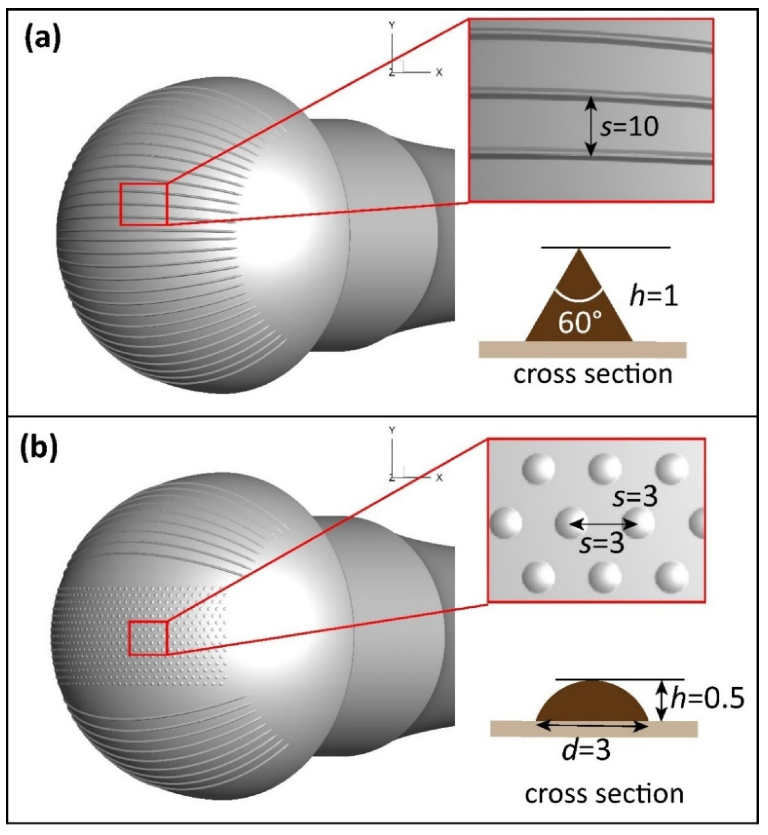
| Helmet Type | Region A and C | Region B | |||||
|---|---|---|---|---|---|---|---|
| Riblets | Riblets | Bump | |||||
| h | s | h | s | h | d | s | |
| Type 1 | 0.5 | 10 | 0.5 | 10 | Null | ||
| Type 2 | 0.5 | 10 | Null | 0.5 | 3 | 6 | |
| Type 3 | 0.5 | 10 | Null | 0.5 | 3 | 4 | |
| Original | Smooth Surface | ||||||
Disclaimer/Publisher’s Note: The statements, opinions and data contained in all publications are solely those of the individual author(s) and contributor(s) and not of MDPI and/or the editor(s). MDPI and/or the editor(s) disclaim responsibility for any injury to people or property resulting from any ideas, methods, instructions or products referred to in the content. |
© 2022 by the authors. Licensee MDPI, Basel, Switzerland. This article is an open access article distributed under the terms and conditions of the Creative Commons Attribution (CC BY) license (https://creativecommons.org/licenses/by/4.0/).
Share and Cite
Wang, Y.; Weng, D.; Wei, Y.; Ma, Y.; Chen, L.; Wang, J. Aerodynamic Drag Reduction on Speed Skating Helmet by Surface Structures. Appl. Sci. 2023, 13, 130. https://doi.org/10.3390/app13010130
Wang Y, Weng D, Wei Y, Ma Y, Chen L, Wang J. Aerodynamic Drag Reduction on Speed Skating Helmet by Surface Structures. Applied Sciences. 2023; 13(1):130. https://doi.org/10.3390/app13010130
Chicago/Turabian StyleWang, Yanqing, Ding Weng, Yuju Wei, Yuan Ma, Lei Chen, and Jiadao Wang. 2023. "Aerodynamic Drag Reduction on Speed Skating Helmet by Surface Structures" Applied Sciences 13, no. 1: 130. https://doi.org/10.3390/app13010130