Traffic Stream Characteristics Analysis for Roadway Linking to Pick-up Zone of Passenger Transportation Hub: A Fundamental Diagram Derived from Threshold Queueing Theory

Abstract

A pick-up zone links a hub of inter-city transportation (e.g., airplane and rail, etc.) with a connected roadway belonging to the city road network. Passengers depart through the pick-up zone and the interactions between passengers and vehicles lead to delays and queues of vehicles on the connected roadway. A better understanding of the unique traffic characteristics of the connected roadway can help to reveal the collecting or dispersing capacity of the hub. This paper treats passenger boarding in a pick-up zone as a service process in a queue system and uses a fundamental diagram model derived from M/M/1 threshold queueing theory with two service phases to investigate the supply–demand relationship of the system. A calibration method is proposed to determine the parameters of the model. Numerical experiments showed that the model can capture a unique capacity drop in the pick-up zone. Moreover, analyses on the impacts of designed parameters on the model features, such as capacity and degree of capacity drop, were performed, and the comparisons showed that the model used performs better than other classical methods with a 0.69 mean squared error and a 0.90 sum of squares due to error). The results will be important supports for hub capacity management.

1. Introduction

As a core link between inter-city transportation (e.g., airplane and rail, etc.) and intra-city transportation (e.g., vehicle and urban rail transit, etc.), hubs play an irreplaceable role in city mobility. Passengers board vehicles in the pick-up zone and depart the hub by a connected roadway. A better understanding of the unique traffic characteristics of the connected roadway can help to reveal the collecting and dispersing capacity of the hub.

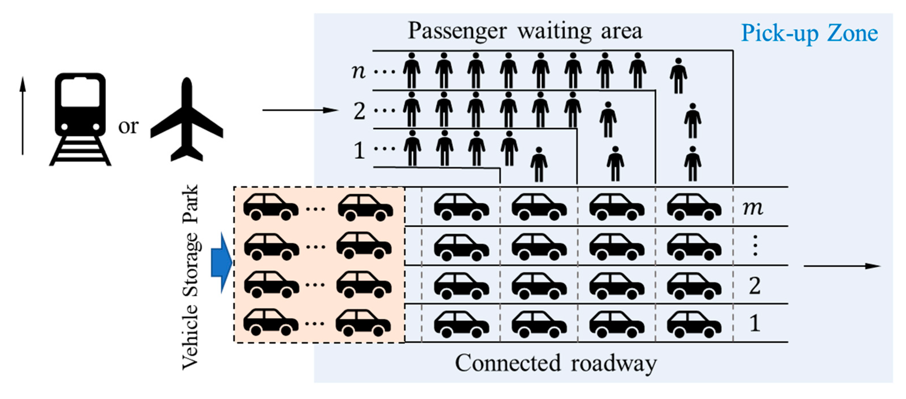
One key element for exploring the traffic characteristics is a consideration of the queues generated in the pick-up zone. Generally, the pick-up zone contains three main parts: the vehicle service area, vehicle queueing area and passenger waiting area. After arrival at the hub by inter-city transportation, passengers walk to the passenger waiting area. Meanwhile, the vehicles leave the vehicle storage park and enter the vehicle service area to pick passengers up using the connected roadway. Because the interactions between passengers and vehicles cost time, delays and queues of vehicles are generated on the roadway. This process is illustrated by Figure 1. The traffic characteristics led by the queuing in the pick-up zone can be seen in the data. In Figure 2, when the vehicle flow density increases over the peak regime, the flow drops sharply along with capacity drops [1]. The capacity of the roadway linking to a hub is thus hard to measure.

Motivated by this, this paper aims to describe the process of human–vehicle interaction in the pick-up zone through a threshold queueing theory model, and from this, to reason about the queuing of vehicles on the connected road and thus assess its capacity. Helbing [2] explained this phenomenon as the transition from non-congested traffic to congested traffic, which inspired our research. Specifically, a fundamental diagram (FD) model derived from M/M/1 threshold queueing theory with two service conditions is used for capturing the traffic characteristics of a roadway connecting to a large-scale hub.

2. Literature Reviews

The characterization and estimation of the road traffic state play an important role in relieving traffic congestion or optimizing the use of the road infrastructure. The traffic impedance (the relationship between vehicle travel time and traffic flow) and the fundamental diagram are theories that characterize the state of traffic. Recently, some new results have emerged from research on the characterization and estimation of the traffic state. For example, Zambrano-Martinez et al. [3] proposed an equation to characterize the relationship between vehicle travel time and traffic flow belonging to the sigmoid family on most of the road sections in the city of Valencia, Spain, which does not fit the general theory of vehicle flow, namely, by applying logistic regression, and the results were able to significantly improve the curve fitting of these road sections. Habtie et al. [4] constructed a real-time traffic state estimation framework for urban roads based on an artificial neural network by acquiring road traffic data with the help of cellular networks. The validation using simulation and real data shows that the model has stable and reliable performance in predicting the real-time traffic condition of urban roads.

The discovery of the basic parameter relationships of traffic flow opened the study of traffic flow theory. The basic diagram describes the interchange relationship of traffic flow, density and speed, and reflects the change in traffic state. Since Greenshields pioneered the study of traffic flow theory, many scholars have studied the shape of the fundamental diagram and proposed a variety of traffic flow models, as shown in Table 1.

Greenshields [5] earlier proposed a linear speed–density relationship model, from which a parabolic-shaped flow–density model can be derived. Greenberg [6] derived a logarithmic speed–density model based on fluid dynamic principles and found that this model is more consistent with the data under traffic congestion. Underwood [7] obtained the exponential speed–density model by studying the measured traffic data, and further study found that it is not applicable to the traffic condition on fast roads, but to less dense traffic situations. The GHR_M1 model is a bell-shaped speed–density model proposed by Drake et al. [8] The model’s estimate of the speed of the free flow is usually lower than the actual value. The GHR_M2 model is a family of model curves proposed by Munjal and Pipes [9] with parameters $n$ greater than 0 and with different shapes for three cases: $n<1$, $n=1$, $n>1$. The Draw model proposed by Draw [10] is similar to the GHR_M2 model in that it introduces an additional parameter that allows for greater degrees of freedom in data fitting. The Kühne and Rödiger model is a model proposed by Kühne and Rödiger [11] to simulate highway traffic under heavy traffic conditions. The model takes into account the relaxation of the static speed and density relationship and the prediction of downstream traffic conditions. The S3 model is an S-shaped speed–density model containing three parameters proposed by Cheng et al. [12] The model is able to describe the relationship between the variation in traffic speed and density on highways under a wide range of possible density conditions. The two-fluid model is a model proposed by Herman and Prigogine [13] based on the kinetic theory of multilane highway traffic for studying the transition of traffic to a collective flow regime under high-density conditions. The car-following model is an application of differential equations to describe the vehicle-following motion law, and the NF model is derived from Newell’s car-following model [14]. The Kerner model was derived by Kerner and Konhäuser [15] based on the non-linear theory of traffic flow clustering effects and the study of static moving cluster structures. The Jayakrishnan model is derived from the link cost function derived by Jayakrishnan et al. [16] using a modified Greenshield model, which is monotonically non-decreasing and convex with respect to density. The Van Aerde model is a single-regime speed–density model proposed by Van Aerde [17] based on a study of congested and non-congested traffic flows on high-speed roadways. The MacNicholas model is a model used by MacNicholas [18] to simulate transit times on long routes. The model contains both deterministic and stochastic components. The 5PL model is a logistic speed–density model containing five parameters proposed by Wang et al. [19] The model achieves the unification of mathematical theory and experiment. The Ni model is a longitudinal control model (LCM) proposed by Ni et al. [20] The model consists of two model representations, macroscopic and microscopic, with the former describing vehicle longitudinal operation control and the latter describing steady-state traffic epidemic behavior. Edie [21] proposes a multi-regime speed–density model that combines the two models based on the different applicability conditions of the Greenberg and Underwood models, using the Greenberg model when traffic density is high and the Underwood model when traffic density is low.

Table 1. Typical fundamental diagrams.

ID	Reference	Equation	Parameters *
1	Greenshields model [5]	$v=v_f·\left(1-k/k_j\right)$	$v_f$, $k_j$
2	Greenberg model [6]	$v=v_c·ln\left(\frac{k_j}{k}\right)$	$v_c$, $k_j$
3	Underwood model [7]	$v=v_f·exp\left(-k/k_c\right)$	$v_f$, $k_c$
4	GHR_M1 model [22]	$v=v_f·exp\left[-{\left(k/k_c\right)}^2/2\right]$	$v_f$, $k_c$
5	GHR_M2 model [22]	$v=v_f·\left[1-{\left(\frac{k}{k_j}\right)}^m\right]$	$v_f$, $k_j$, $m$
6	GHR_M3 model [22]	$v=v_f·{\left(1-\frac{k}{k_j}\right)}^m$	$v_f$, $k_j$, $m$
7	Drew model [10]	$v=v_f\left(1-{\left(\frac{k}{k_j}\right)}^{n+\frac{1}{2}}\right)$	$k_j$, $n$
8	Kühne and Rödiger model [11]	$v=v_f{\left(1-{\left(\frac{k}{k_j}\right)}^a\right)}^b$	$k_j$, $a$, $b$
9	S3 model [12]	$v=v_f{\left[1+{\left(\frac{k}{k_c}\right)}^m\right]}^{-\frac{2}{m}}$	$v_f$, $k_c$, $m$
10	Two-fluid model [13]	$v=v_f·{\left[1-{\left(\frac{k}{k_j}\right)}^p\right]}^{n+1}$	$v_f$, $k_j$, $p$, $n$
11	NF model [14]	$v=v_f·\left[1-exp\left(-\frac{\lambda }{v_f}\left(\frac{1}{k}-\frac{1}{k_j}\right)\right)\right]$	$v_f$, $k_j$, $\lambda$
12	Kerner model [15]	$v=v_f\left[\frac{1}{\left(1+exp\left(\frac{1}{c_2}\left(\frac{k}{k_c-c_1}\right)\right)\right)}-c_3\right]$	$v_f$, $k_c$, $c_1$, $c_2$, $c_3$
13	Jayakrishnan model [16]	$v=v_j+\left(v_f-v_j\right)·{\left(1-k/k_j\right)}^m$	$v_f$, $v_j$, $k_j$, $m$
14	Van Aerde model [17]	$k=1/\left(c_1+\frac{c_2}{v_f-v}+c_3·v\right)$	$v_f$, $c_1$, $c_2$, $c_3$
15	MacNicholas model [18]	$v=v_f·\left[\frac{k_j^m-k^m}{k_j^m+c·k^m}\right],m\ge 1,c\ge 0$	$v_f$, $k_j$, $m$, $c$
16	5PL model [19]	$v=v_j+\frac{v_f-v_j}{{\left\{1+exp\left[\left(k-k_c\right)/{\theta }_1\right]\right\}}^{{\theta }_2}}$	$v_f$, $v_j$, $k_c$, ${\theta }_1$, ${\theta }_2$
17	Ni model [20]	$k=\frac{1}{\left(\gamma v^2+\tau v+l\right)\left[1-ln\left(1-v/v_f\right)\right]}$	$v_f$, $\gamma$, $\tau$, $l$
18	Edie model [21]	$v=\left\{\begin{array}{c}{v}_f·exp\left(-k/k_c\right),k\le k_c\\ v_c·\ln \left(k_j/k\right),k>k_c\end{array}\right.$	$v_f$, $k_c$, $v_c$, $k_j$

* We denote $v_c$ and $k_c$ as the speed and density at the maximum flow. Furthermore, let $v_j$ denote the minimal speed at jam density.

Table 1. Typical fundamental diagrams.

ID	Reference	Equation	Parameters *
1	Greenshields model [5]	$v=v_f·\left(1-k/k_j\right)$	$v_f$, $k_j$
2	Greenberg model [6]	$v=v_c·ln\left(\frac{k_j}{k}\right)$	$v_c$, $k_j$
3	Underwood model [7]	$v=v_f·exp\left(-k/k_c\right)$	$v_f$, $k_c$
4	GHR_M1 model [22]	$v=v_f·exp\left[-{\left(k/k_c\right)}^2/2\right]$	$v_f$, $k_c$
5	GHR_M2 model [22]	$v=v_f·\left[1-{\left(\frac{k}{k_j}\right)}^m\right]$	$v_f$, $k_j$, $m$
6	GHR_M3 model [22]	$v=v_f·{\left(1-\frac{k}{k_j}\right)}^m$	$v_f$, $k_j$, $m$
7	Drew model [10]	$v=v_f\left(1-{\left(\frac{k}{k_j}\right)}^{n+\frac{1}{2}}\right)$	$k_j$, $n$
8	Kühne and Rödiger model [11]	$v=v_f{\left(1-{\left(\frac{k}{k_j}\right)}^a\right)}^b$	$k_j$, $a$, $b$
9	S3 model [12]	$v=v_f{\left[1+{\left(\frac{k}{k_c}\right)}^m\right]}^{-\frac{2}{m}}$	$v_f$, $k_c$, $m$
10	Two-fluid model [13]	$v=v_f·{\left[1-{\left(\frac{k}{k_j}\right)}^p\right]}^{n+1}$	$v_f$, $k_j$, $p$, $n$
11	NF model [14]	$v=v_f·\left[1-exp\left(-\frac{\lambda }{v_f}\left(\frac{1}{k}-\frac{1}{k_j}\right)\right)\right]$	$v_f$, $k_j$, $\lambda$
12	Kerner model [15]	$v=v_f\left[\frac{1}{\left(1+exp\left(\frac{1}{c_2}\left(\frac{k}{k_c-c_1}\right)\right)\right)}-c_3\right]$	$v_f$, $k_c$, $c_1$, $c_2$, $c_3$
13	Jayakrishnan model [16]	$v=v_j+\left(v_f-v_j\right)·{\left(1-k/k_j\right)}^m$	$v_f$, $v_j$, $k_j$, $m$
14	Van Aerde model [17]	$k=1/\left(c_1+\frac{c_2}{v_f-v}+c_3·v\right)$	$v_f$, $c_1$, $c_2$, $c_3$
15	MacNicholas model [18]	$v=v_f·\left[\frac{k_j^m-k^m}{k_j^m+c·k^m}\right],m\ge 1,c\ge 0$	$v_f$, $k_j$, $m$, $c$
16	5PL model [19]	$v=v_j+\frac{v_f-v_j}{{\left\{1+exp\left[\left(k-k_c\right)/{\theta }_1\right]\right\}}^{{\theta }_2}}$	$v_f$, $v_j$, $k_c$, ${\theta }_1$, ${\theta }_2$
17	Ni model [20]	$k=\frac{1}{\left(\gamma v^2+\tau v+l\right)\left[1-ln\left(1-v/v_f\right)\right]}$	$v_f$, $\gamma$, $\tau$, $l$
18	Edie model [21]	$v=\left\{\begin{array}{c}{v}_f·exp\left(-k/k_c\right),k\le k_c\\ v_c·\ln \left(k_j/k\right),k>k_c\end{array}\right.$	$v_f$, $k_c$, $v_c$, $k_j$

* We denote $v_c$ and $k_c$ as the speed and density at the maximum flow. Furthermore, let $v_j$ denote the minimal speed at jam density.

A number of scholars have studied FD from a queuing perspective. The traffic speed–density model derived based on the queuing model is shown in

Table 2. Typical queueing-based fundamental diagrams.

Reference	Queueing Type	The Derived Fundamental Diagram	Notes
Vandaele et al. [23]	M/M/1	$v=v_f·\left(1-\rho \right)$	$\rho =\frac{\lambda }{\mu }=\frac{k}{k_j}$
Heidemann [24]	M/G/1	$v=\frac{2v_f·\left(1-\rho \right)}{2+\rho ·\left({\beta }^2-1\right)}$	$\beta =\sigma ·v_f·k_j$
Jain and Smith [25]	M/G/c/c	$V_n=\frac{v_f}{C}\left(C+1-n\right)$	$C=k_j·L·N$
	M/G/c/c	$V_n=v_f·exp\left[-{\left(\frac{n-1}{\beta }\right)}^{\gamma }\right]$	note 1
Vandaele et al. [23]	G/G/1	$v=\frac{2v_f·\left(1-\rho \right)}{2\left(1-\rho \right)+\rho \left(c_a{}^2+c_s{}^2\right)exp\left(\frac{-2\left(1-\rho \right){\left(1-c_a{}^2\right)}^2}{3\rho \left(c_a{}^2+c_s{}^2\right)}\right)}$	$c_a{}^2\le 1$
	G/G/1	$v=\frac{2v_f·\left(1-\rho \right)}{2\left(1-\rho \right)+\rho \left(c_a{}^2+c_s{}^2\right)exp\left(\frac{-\left(1-\rho \right){\left(c_a{}^2-1\right)}^2}{\left(1+\rho \right)\left(c_a{}^2+10c_s{}^2\right)}\right)}$	$c_a{}^2>1$
Van Woensel et al. [26]	G/G/zK	$v=\frac{2v_f·z\left(1-\rho \right)}{2z\left(1-\rho \right)+\rho \left(c_a{}^2+c_s{}^2\right)\left(\sqrt{2\left(z+1\right)}-1\right)}$	note 2
	G/G/zW	$v=\frac{2v_f}{2+\varphi \left(c_a{}^2+c_s{}^2\right)W_{qM/M/z}}$	note 3

¹$\gamma$, $\beta$ are parameters. ² $z$ is the number of servers. ³ $\varphi$ is a correction factor defined in Whitt [27] and $W_{qM/M/z}$ is a formula for the waiting time in an $M/M/z$ queue proposed by Vandaele et al. [23].

. Vandaele et al. [23] derived the traffic speed–density model for this type of queuing system based on the formula for calculating the mean sojourn time in M/M/1 queuing systems. Heidemann [24] considered the M/G/1 queuing system and analyzed the queuing process of vehicles, proposed a correlation formula between traffic parameters and queuing system parameters, and derived the traffic speed–density model of the M/G/1 queuing system based on the Pollaczek–Khintchine formula. Jain and Smith [25] used the M/G/c/c queuing model to model and analyze traffic flow and proposed linear and exponential models describing the relationship between traffic speed and roadway capacity $C$ ($C$ is related to roadway length $L$ and number of lanes $N$) and the number of vehicles $n$. Vandaele et al. [23] used a G/G/1 queuing model to model traffic flow and derived a traffic speed–density model based on the Little and Kraemer–Lagenbach-Belz formulas, which contains a coefficient of variation $c_a{}^2$ for the vehicle arrival interval time and a coefficient of variation $c_s{}^2$ for the service time, with the type of model depending on the magnitude of $c_a{}^2$ relative to 1.

Existing studies have proved that the queuing model can appropriately simulate the traffic flow of the road section, Based on the queuing theory, the characteristics of traffic flow can be studied. The influence of the behavior of the traffic flow on the road section on the macroscopic characteristics can be analyzed from a more detailed level. The traffic flow model derived from queuing theory is also more advantageous in MFD curve sensitivity analysis. Nevertheless, how to model and how to calibrate the corresponding multiresolution parameters still remains a challenge.

The rest of this paper is organized as follows: Section 3 illustrates details of the methodology used, including how the queueing model and the FD models are built based on the properties of the roadway connecting to the transportation hub pick-up zone, as well as the measurement methods of the parameters at different resolutions. Section 4 analyzes the basic characteristics of the model and compares the performance with other models using a set of numerical experiments.

3. Methodology

A fundamental diagram model derived from M/M/1 threshold queueing theory with two service conditions (i.e., congested and non-congested) is used for capturing the unique traffic characteristics of roadway connecting to transportation hub. This model takes human–vehicle interaction as a process of serving vehicles, where the service rate is controlled by the condition of queuing system. If the queue is in a non-congested condition, the service rate is high. Otherwise, if queuing system converts to congested condition, the service is performed with a low service rate [28,29].

Before modeling, the variables and parameters involved in this model are defined in

Table 3. Overview of used variables and parameters in the model.

	Resolution	Notation	Type	Description
1	Macroscopic	$q$	Variable	Traffic flow (veh/min)
2		$q_b$		Traffic flow by batches (batches/min)
3		$k$		Traffic density (veh/m)
4		$k_b$		Traffic density by batches (batches/m)
5		$v$		Traffic speed (m/min)
6		$k_j$	Parameter	Maximum traffic density (veh/m)
7		$k_{bj}$		Maximum traffic density by batches (batches/m)
8		$v_f$		Maximum traffic speed (m/min)
9		$q_{max}$		The maximum of traffic flow (veh/min)
10	Mesoscopic	${\lambda }_b$	Parameter	Arrival rate of intra-city transportation vehicle by batch (batches/min)
11		${\mu }_b$		Service rate of vehicle queue by batches (batches/min)
12		${\mu }_1$		Service rate in non-congested condition (veh/min)
13		${\mu }_{b1}$		Service rate in non-congested condition by batch (batches/min)
14		${\mu }_2$		Service rate in congested condition (veh/min)
15		${\mu }_{b2}$		Service rate in congested condition by batch (batch/min)
16		${\rho }_{b1}$		Service load rate in non-congested situation by batch
17		${\rho }_{b2}$		Service load rate in congested situation by batch
18		${\lambda }_p$		Arrival rate of passenger (per/min)
19		${\lambda }_a$		Arrival rate of inter-city transportation vehicle (veh/min)
20		$m$		Number of vehicle lanes
21		$l$		Length of roadway
22		$N$		Buffer of single vehicle lane
23		$n$		Number of passenger lanes in queue
24		$C$		Passing capacity of the connected roadway
25		$k_C$		Critical density of the connected roadway
26		${\phi }_d$		Degree of capacity drop
27		$\mathsf{\Lambda }$		Effective arrival rate (veh/min)
28		$U$		Threshold number of vehicles at which the vehicle queue becomes congested
29		$U_b$		Threshold number of batches at which the vehicle queue becomes congested
30		$D$		Threshold number of vehicles at which the vehicle queue becomes non-congested
31		$D_b$		Threshold number of batches at which the vehicle queue becomes non-congested
32		$\pi \left(i,j\right)$		The probability that vehicle queue length is $i$ under state $j$
33		$S$	Variable	The service time of a vehicle (min)
34		$S_b$		The service time of a batch of vehicles (min)
35		$E\left(S\right)$		The mean sojourn time of each vehicle in the queue
36		$E_b\left(E\right)$		The mean sojourn time of each batch of vehicles in the queue

.

3.1. A Batch-Based Queueing Model for Passenger–Vehicle Interaction in the Pick-up Zone

There are passenger queue and vehicle queue both constrained by storage buffer existing in the pick-up zone and the connected roadway. The passenger queue is set in the passenger waiting area with $n$ passenger waiting lanes and the vehicle queue is set across the vehicle storage park and vehicle service area with $m$ lanes in the pick-up zone. We denote the length of connected roadway as $l$. Vehicles of inter-city transportation arrive at the passenger transportation hub at a rate ${\lambda }_a$, and passengers leave the hub and arrive at the passenger queue at rate ${\lambda }_p$. Because of the management rules, we assume that vehicles move to the pick-up zone in batches (i.e., branch by branch of vehicles) from the vehicle storage park and leave in batches after carrying passengers. We set the vehicle queue has finite buffer $N$ in batch. Based on these, we abstract the vehicle queuing process into a batch-based queue, as shown in Figure 3.

As vehicles are served in batches in the queuing system, there is a transformation between the actual traffic parameters within the connected roadway and the traffic parameters in the vehicle queuing system in terms of quantity units; specifically, when the traffic flow of the connected roadway is $q$, the traffic density is $k$, and the maximum traffic density is $k_j$. The relationship between the traffic flow $q_b$, the traffic density $k_b$ and the maximum traffic density $k_{bj}$ of the vehicle queuing system and $q$, $k$ and $k_j$ are as Equation (1):

$$q_b=\frac{q}{\left(n·m\right)} , k_b=\frac{k}{\left(n·m\right)}, k_{bj}=\frac{k_j}{\left(n·m\right)}$$

(1)

For the vehicle queue, vehicles are serviced in the vehicle service area and the queue is placed across both the roadway and the vehicle storage park. We assume that each batch of vehicles arrives under a Poisson process, which follows an exponential distribution with parameter ${\lambda }_b$ (i.e., the rate of each batch of vehicles arriving at the passenger transportation hub is ${\lambda }_b$). The service rate in the vehicle service area is ${\mu }_b$, which also follows an exponential distribution. Because of the interactions between vehicles, we assume that there are two conditions of the vehicle queue: non-congested condition and the congested condition. The transition between these two conditions is controlled by the vehicle queue length, and the values of ${\mu }_b$ are taken according to the different conditions.

The mean sojourn time $E_b\left(S\right)$ of each batch of vehicles in the queue includes the waiting time and the service time in the vehicle service area. If the number of vehicle batches in the single vehicle lane reaches $N$, the traffic flow in the connected roadway is blocked, and the traffic density at this time is the maximum density $k_{bj}$. According to the definition of the maximum density, $1/k_{bj}$ is the minimum length each batch of vehicles requires. We set $1/k_{bj}$ as the length of the vehicle service area. The time consumed by each batch of vehicles to completely pass through the vehicle service area is $E_b\left(S\right)$, so the speed $v$ of each batch of vehicles in the connected roadway is as shown in Equation (2):

$$v=\frac{1/k_{bj}}{E_b\left(S\right)}=\frac{n·m}{k_j·E_b\left(S\right)}$$

(2)

3.2. Threshold Queuing Model Based on M/M/1

The queuing process of vehicles in the connected roadway is represented by an M/M/1 threshold queuing model. According to the characteristics of the threshold queue, each batch of vehicles arrives at the passenger transportation hub at an average interval of $1/{\lambda }_b$. In the initial stage, the traffic flow is small, the traffic in the connected roadway is in a non-congested condition and the vehicles can drive away from the pick-up zone with passengers faster, and the average time consumed by each batch of vehicles in the vehicle service area is $1/{\mu }_{b1}$. With the increase in traffic flow, the length of the vehicle queue in the connected roadway gradually increases. After the number of batches of vehicles in the queue exceeds a certain value $U_b$, the traffic flow in the connected roadway is in a congested condition; at this stage, the time consumed by each batch of vehicles to carry passengers and leave the pick-up zone is also extended to $1/{\mu }_{b2}$. With the continuous dissipation of passengers and vehicles, the length of the vehicle queue gradually shortens. After the number of batches of vehicles in the queue is reduced to a certain value $D_b$, the traffic flow in the connected roadway is once again in a non-congested condition. The average time consumed by vehicles in the vehicle service area also decreases back to $1/{\mu }_{b1}$.

The transition between non-congested and congested conditions is controlled by a low threshold $D_b$ and a high threshold $U_b$. When the number of batches of queuing vehicles is less than $D_b$, the service rate of the vehicle service area is higher and follows the exponential distribution with parameter ${\mu }_{b1}$. When the number of batches of queuing vehicles is greater than $U_b$, the service rate of the vehicle service area is lower and follows the exponential distribution with parameter ${\mu }_{b2}$. When the number of batches of queuing vehicles is between $\left(D_b, U_b\right)$, two service rates of ${\mu }_{b1}$ and ${\mu }_{b2}$ exist simultaneously. The condition transition process of the vehicle queue controlled by the threshold is shown in Figure 4.

According to Markov chain [30], the probability of the queue length when the system reaches the steady state can be obtained. Let $\pi \left(i, j\right)$ denote the probability that the queue length of the queue is $i$ in state $j \left(j=1,2\right)$, with $j=1$ indicating that the system is in the non-congested state and $j=2$ indicating that it is in the congested state. The service load rate of the vehicle service area in the non-congested condition is ${\rho }_{b1}={\lambda }_b/{\mu }_{b1}$, and the service load rate in the congested condition is ${\rho }_{b2}={\lambda }_b/{\mu }_{b2}$, then the steady-state probability of the system can be obtained from Equations (3)–(6).

$$\pi \left(i,1\right)=\pi \left(0,1\right){\rho }_{b1}{}^i, i=1,2,\dots ,D_b-1$$

(3)

$$\pi \left(i,1\right)=\pi \left(0,1\right)\frac{{\rho }_1{}^i-{\rho }_{b1}{}^{U_b+1}}{1-{\rho }^{U_b-L_b+2}}, i=D_b,D_b+1,\dots ,U_b$$

(4)

$$\pi \left(i,2\right)=\pi \left(0,1\right)\frac{{\rho }_{b2}-{\rho }_{b2}{}^{i-D_b+2}}{1-{\rho }_{b2}}\frac{{\rho }_{b1}{}^{U_b}-{\rho }_{b1}{}^{U_b+1}}{1-{\rho }_{b1}{}^{U_b-D_b+2}}, i=D_b,D_b+1,\dots ,U_b$$

(5)

$$\pi \left(i,2\right)=\pi \left(0,1\right)\frac{{\rho }_{b2}{}^{i-U_b}-{\rho }_{b2}{}^{i-D_b+2}}{1-{\rho }_{b2}}\frac{{\rho }_{b1}{}^{U_b}-{\rho }_{b1}{}^{U_b+1}}{1-{\rho }_{b1}{}^{U_b-D_b+2}}, i=U_b+1,\dots ,N$$

(6)

where $\pi \left(0,1\right)$ can be found according to the regularity condition shown in Equation (7):

$$\sum _{i=0}^{U_b}\pi \left(i,1\right)+\sum _{i=D_b}^N\pi \left(i,2\right)=1$$

(7)

Based on Little’s law [31], the mean sojourn time of each batch of vehicles in the queue is shown in Equation (8):

$$E_b\left(S\right)=\frac{1}{\mathsf{\Lambda }}\left(\sum _{i=0}^{U_b}i·\pi \left(i,1\right)+\sum _{i=D_b}^{N}i·\pi \left(i,2\right)\right)$$

(8)

where $\mathsf{\Lambda }$ is the effective arrival rate of the queue, and Equation (9):

$$\mathsf{\Lambda }=\lambda \left(\sum _{i=0}^{U_b}\pi \left(i,1\right)+\sum _{i=D_b}^{N-1}\pi \left(i,2\right)\right)=\lambda \left(1-\pi \left(N,2\right)\right)$$

(9)

According to Equation (2), Equations (10)–(12) in Heidemann’s Model [24] are:

$$q_b=k_b·v$$

(10)

$${\lambda }_b=k_b·v_f$$

(11)

$$k_b=\left(1-\pi \left(0,1\right)\right)k_{bj}$$

(12)

We obtain Equation (13):

$$\begin{array}{l}{q}_b=\frac{k_b}{k_{bj}·E_b\left(S\right)}=\frac{k_b·\mathsf{\Lambda }}{k_{bj}\left({\sum }_{i=0}^{U_b}i·\pi \left(i,1\right)+{\sum }_{i=D_b}^{N}i·\pi \left(i,2\right)\right)}\\ =\frac{k_b·{\lambda }_b\left(1-\pi \left(N,2\right)\right)}{k_{bj}\left({\sum }_{i=0}^{U_b}i·\pi \left(i,1\right)+{\sum }_{i=D_b}^{N}i·\pi \left(i,2\right)\right)}\\ =\frac{k_b{}^2·v_f\left(1-\pi \left(N,2\right)\right)}{k_{bj}\left({\sum }_{i=0}^{U_b}i·\pi \left(i,1\right)+{\sum }_{i=D_b}^{N}i·\pi \left(i,2\right)\right)}\end{array}$$

(13)

3.3. Calibration Method for Parameters of the Model

Due to the abstraction of the traffic flow in the connected roadway, the vehicles in the queueing system are in batches as the basic unit, and the variables and parameters in the traffic flow model Equation (13) derived based on the queueing model are also in batches as the basic unit. The actual observed traffic flow data are all in the basic unit of vehicle. Therefore, to fit Equation (13) based on the actual observed data, it is necessary to convert Equation (13) to Equation (14).

$$q=\frac{k^2·v_f\left(1-\pi \left(N,2\right)\right)}{k_j\left({\sum }_{i=0}^{U}i·\pi \left(i,1\right)+{\sum }_{i=D}^{N}i·\pi \left(i,2\right)\right)}$$

(14)

The transformation relationship between the variables $q$ and $k$ of Equation (14) and $q_b$ and $k_b$ is shown in Equation (1). The parameters of Equation (14) include $k_j$, $v_f$, ${\mu }_1$, ${\mu }_2$, $D$ and $U$. The relationship between the parameters $k_j$ and $k_{bj}$ is shown in Equation (1), while $k_{bj}$ can be determined by $N$ and $l$ with $1/k_{bj}=l/\left(N+1\right)$, so $k_j$ can be determined by Equation (15).

$$k_j=\frac{n·m·\left(N+1\right)}{l}$$

(15)

In addition, $v_f$ can be obtained from actual observation and can be taken as $v_f=$200 m/min. The transformation relationship between parameters ${\mu }_1$, ${\mu }_2$, $D$ and $U$ and ${\mu }_{b1}$, ${\mu }_{b2}$, $D_b$ and $U_b$ is shown in Equation (16).

$${\mu }_{b1}={\mu }_1/\left(n·m\right), {\mu }_{b2}={\mu }_2/\left(n·m\right), D_b=D/\left(n·m\right), U_b=U/\left(n·m\right)$$

(16)

The parameters to be fitted to Equation (16) are ${\mu }_1$, ${\mu }_2$, $D$ and $U$. In this paper, the least squares method is used for the fitting [32].

4. Numerical Experiments

In order to obtain traffic data and analyze the influence of the design parameters of the pick-up zone of the hub on the connected roadway traffic characteristics, we built a simulation model based on the Anylogic simulation platform to simulate the queuing of passengers waiting for vehicles in the pick-up zone of the hub and the queuing of vehicles carrying passengers in the connected roadway.

Anylogic is a modeling tool based on the latest advances in modeling science and information technology over the past years and is suitable for modeling and simulation in a wide range of industries, such as supply chain, manufacturing, transportation, warehouse operations, rail logistics, etc. The simulation software supports intelligent agent-based, system dynamics and discrete-event modeling approaches as well as multimethod hybrid modeling.

The hub simulation model constructed in this paper is based on agent-based and discrete-event modeling, and the three main types of agents are inter-city traffic vehicles (we use aircraft and train agents), pedestrians and cars agents. The simulation process includes behaviors or scenarios such as aircraft or train arrivals and departures; passengers arriving at the hub choosing to board or take the train; passengers landing or arriving at the hub choosing to leave directly or wait in the passenger waiting area, leaving by public transportation; and vehicles arriving at the vehicle storage park in the connected roadway of the hub and driving from the storage park to the vehicle serving area, carrying passengers and then leaving. We analyzed the traffic characteristics of the traffic flow in the connected roadway, so we measured the traffic flow, average density and average speed in the roadway every 10 min during the simulation. The simulation duration was set to one week, and the obtained traffic data were analyzed. Using simulation, we carried out the following work:

(1)

We changed the design parameters of the hub (including the arrival rate of inter-city transportation vehicle ${\lambda }_a$, number of passenger queues $n$, number of lanes $m$ and buffer of single vehicle lane $N$) to set several simulation schemes. Then we obtained the different flow–density–speed data, fitting parameters (including the service rate of non-congested status ${\mu }_1$, service rate of congested status ${\mu }_2$, threshold at congested $U$ and threshold at non-congested $D$) by fitting the model shown in Equation (13), and obtained measurement results (including the capacity of the connected roadway $C$, critical density of capacity $k_C$ and the degree of capacity drop ${\phi }_d$).

(2)

We analyzed the influence and tendency of different design parameters on the fitting parameters, measurement results and fitting curve shape.

(3)

We selected other classical models for fitting the flow–density–speed data, and compared their errors and fitness in different areas. It verified the advantages and effectiveness of our model in describing the unique traffic characteristics of the inter-city hub connection roadway.

(4)

In order to analyze the sensitivity of fitting parameters, we changed the values of each fitting parameter of the benchmark and obtained the measurement results. Then we analyzed the influence and tendency of different fitting parameters on the measurement results and fitting curve shape.

4.1. Experiment Design

Based on the simulation model, we took the design parameters ${\lambda }_a=0.06, n=3, m=2, N=165$ as the benchmark, changed the values of each design parameter separately to form a total of four groups of design parameter value schemes for simulation experiments. Each group includes different values of three corresponding design parameters, as shown in the first four rows of

Table 4. Design parameters and corresponding results to different schemes.

Parameters and Results		Benchmark	Group 1 $\left({\lambda }_a\right)$			Group 2 $\left(n\right)$			Group 3 $\left(m\right)$			Group 4 $\left(N\right)$
Design parameters	${\mathit{\lambda }}_{\mathit{a}}$	0.06	0.04	0.05	1.00	0.06	0.06	0.06	0.06	0.06	0.06	0.06	0.06	0.06
	$\mathit{n}$	3	3	3	3	2	5	7	3	3	3	3	3	3
	$\mathit{m}$	2	2	2	2	2	2	2	1	3	4	2	2	2
	$\mathit{N}$	165	165	165	165	165	165	165	165	165	165	145	195	215
Fitting parameters	${\mathit{\mu }}_{\mathit{1}}$	452.2	457.3	448.8	454.5	409.7	528.1	576.8	412.6	507.2	564.1	407.7	514.6	566.4
	${\mathit{\mu }}_{\mathit{2}}$	266.6	348.8	307.3	214.2	294.6	227.9	205.2	231.2	295.4	314.4	251.5	286.7	273.3
	$\mathit{D}$	577	522	656	750	683	495	428	549	629	696	564	576	598
	$\mathit{U}$	816	782	839	885	839	782	736	747	857	902	736	908	989
Measurement results	$\mathit{C}$	91.53	93.33	94.58	93.51	75.15	97.74	108.4	79.55	98.75	105.1	74.19	96.94	107.3
	${\mathit{k}}_{\mathit{C}}$	0.888	0.852	0.936	0.960	0.768	0.876	0.996	0.828	0.936	0.972	0.684	0.960	1.032
	${\mathit{\phi }}_{\mathit{d}}$ *	281.9	726.6	159.7	73.00	39.46	198.5	704.0	216.6	174.4	100.2	242.3	227.4	217.6

*${\phi }_d$: The average degree of capacity drops when the flow drops from the maximum to 60 veh/min.

.

Then we carried out simulations to obtain groups of flow–density–speed data in the roadway, and fitted the model shown in Equation (13) to obtain the fitting parameters (${\mu }_1, {\mu }_2,D$ and $U$), as shown in the middle four rows of Table 4. The measurement results ($C,k_C,$ and ${\phi }_d$) of fitting are also shown in the last four rows of Table 4.

4.2. Influence of Pick-Up Zone Design Parameters

According to the parameter values of each group, we drew the fundamental diagram on a flow–density plane with the corresponding fitting curve under different design parameters in Figure 5. It can be seen that the changing the different design parameters will affect $C, k_C$ and ${\phi }_d$.

Then we observed and analyzed the change in and influence of the curve shape, fitting parameters and measurement results when a design parameter in the same group increased, where the degree of capacity drop ${\phi }_d$ is expressed as the average degree of capacity drop when the flow drops from the maximum to a constant (e.g., 60 veh/min). The fitting parameters and the measurement results of each scheme are shown in the last eight rows of Table 4.

From Figure 5a and Table 4, it can be seen that with ${\lambda }_a$ increasing from 0.4 to 1.0, the corresponding fitting parameter ${\mu }_1$ fluctuates between $\left[448.8, 457.3\right]$. ${\mu }_2$ decreases from 348.8 to 214.2. $D$ increases from 522 to 750. $U$ increases from 782 to 885. In the meantime, $C$ fluctuates between $\left[91.53, 94.58\right]$. $k_C$ increases from 0.852 to 0.960. ${\phi }_d$ decreases from 726.6 to 73.0.

From Figure 5b and Table 4, it can be seen that with $n$ increasing from 2 to 7, the corresponding fitting parameter ${\mu }_1$ increases from 409.7 to 576.8. ${\mu }_2$ decreases from 294.6 to 205.2. $D$ decreases from 683 to 428. $U$ decreases from 839 to 736. In the meantime, $C$ increases from 75.15 to 108.4. $k_C$ increases from 0.768 to 0.996. ${\phi }_d$ increases from 29.46 to 704.0.

From Figure 5c and Table 4, it can be seen that with $m$ increasing from 1 to 4, the corresponding fitting parameter ${\mu }_1$ increases from 412.6 to 564.1. ${\mu }_2$ increases from 231.2 to 314.4. $D$ increases from 549 to 696. $U$ increases from 747 to 902. In the meantime, $C$ increases from 79.55 to 105.1. $k_C$ increases from 0.828 to 0.972. ${\phi }_d$ decreases from 216.6 to 100.2.

From Figure 5d and Table 4, it can be seen that with $N$ increasing from 145 to 215, the corresponding fitting parameter ${\mu }_1$ increases from 407.7 to 566.4. ${\mu }_2$ increases from 251.5 to 273.3. $D$ increases from 564 to 598. $U$ increases from 736 to 989. In the meantime, $C$ increases from 74.19 to 107.3. $k_C$ increases from 0.684 to 1.032. ${\phi }_d$ decreases from 242.3 to 217.6.

4.3. Model Comparisions

This section compares the fitting effect of the traffic density model derived from the queue based on threshold control with other models. We take the flow–density-speed data under the benchmark, fitting the Edie’s model [21] and NF model [14] in Table 1, and Heidemann model [24] and Vandaele model [23] in Table 2 ($c_a{}^2\le 1$).

The comparison of the model fitting effect includes fitting errors (including MSE, SSE, MAE and RMSE), fitness (R-square) and measurement results. For fitness, we calculate not only the global fitness but also the local fitness, including the low-density area ($0\le k<0.96$), middle-density area ($0.96\le k<1.44$) and high-density area ($k\ge 1.44$). The results are shown in

Table 5. The fitting errors index of different models. Numbers in bold indicate the minimum error or maximum fitness. (Design parameters: ${\lambda }_a=0.06, n=3, m=2, N=165$.)

Errors, Fitness and Results		Our Model	Heidemann Model	Vandaele Model	Edie Model	NF Model
Fitting errors	MSE	0.81	1.33	1.17	1.47	1.23
	SSE	566.9	927.1	817.0	1025.5	855.0
	MAE	0.69	0.75	0.73	0.9	0.78
	PMSE	0.90	1.15	1.08	1.21	1.11
Fitness * (R-square)	G	0.74	0.57	0.62	0.53	0.61
	L	0.82	0.56	0.75	0.71	0.72
	M	0.77	0.68	0.74	0.73	0.73
	H	−1.97	−9.02	−7.71	−7.65	−7.43
Measurement results	$C$	91.54	72.98	83.52	81.50	81.07
	$k_C$	0.888	0.912	0.768	0.660	0.780
	${\phi }_d$	281.927	16.138	28.404	22.398	24.734

* G = global; L = low-density area; M = middle-density area; H = high-density area.

.

Then we plotted the comparison figure, as shown in Figure 6.

From Table 5 and Figure 6, it can be seen that the fitting errors (MSE, SSE, MAE and RMSE) of our model are the smallest of all models, which indicates that our model has better adaptability on the fitting data.

According to the comparison of R-square, our model has the best fit with the highest global fitness and is greater than 0.7. In addition, the fitness is highest in the low-density and middle-density regions, 0.82 and 0.77, respectively, but the fitness is lower in the high-density region. This indicates that, compared with other models, our model has a better fit in the low-density and middle-density regions but a poor fit in the high-density region (the fitness of all models in the low-density region is less than 0, which shows that all models have this problem).

In addition, the proposed model can capture the capacity point and the capacity drop phenomenon better than other models, which indicates that our model can better reflect the actual capacity of the system.

4.4. Sensitivity Analysis

We gave a set of parameters to build the models and compared them to the results of the benchmark (${\lambda }_a=0.06, n=3, m=2, N=165,{\mu }_1=450,{\mu }_2=270,D=580,U=820$), and formed a total of four groups of given parameters adjustment schemes for a sensitivity analysis of the FD curves. We obtained the measurement results based on each group of given parameters’ values, as shown in

Table 6. Results of given parameters for sensitivity analysis. (Design parameters: ${\lambda }_a=0.06, n=3, m=2, N=165$.)

Parameters and Results		Benchmark	${\mu }_1$			${\mu }_2$			$D$			$U$
Given parameters	${\mu }_1$	450	330	390	510	450	450	450	450	450	450	450	450	450
	${\mu }_2$	270	270	270	270	150	210	360	270	270	270	270	270	270
	$D$	580	580	580	580	580	580	580	460	520	640	580	580	580
	$U$	820	820	820	820	820	820	820	820	820	820	700	760	880
Measurement results	$C$	91.53	74.64	82.88	100.6	91.47	91.53	91.53	91.43	91.51	91.54	90.98	91.50	91.52
	$k_C$	0.888	0.804	0.840	0.924	0.862	0.888	0.888	0.859	0.888	0.888	0.840	0.888	0.888
	${\phi }_d$	281.9	133.7	211.8	323.5	441.2	350.5	216.5	541.7	411.8	138.4	320.7	310.0	245.0

.

Then we plotted the comparison figure, as shown in Figure 7.

From Figure 7a and Table 6, it can be seen that with ${\mu }_1$ in the process of increasing from 330 to 510, the corresponding measurement result $C$ increases from 74.64 to 100.6; $k_C$ increases from 0.804 to 0.924; and ${\phi }_d$ increases from 133.7 to 323.5.

From Figure 7b and Table 6, it can be seen that with ${\mu }_2$ in the process of increasing from 150 to 360, the corresponding measurement result $C$ fluctuates between $\left[91.47, 91.53\right]$; $k_C$ fluctuates between $\left[0.862, 0.888\right]$; and ${\phi }_d$ decreases from 441.2 to 216.5.

From Figure 7c and Table 6, it can be seen that with $D$ in the process of increasing from 460 to 640, the corresponding measurement result $C$ increases from 91.43 to 91.54; $k_C$ increases from 0.859 to 0.888; and ${\phi }_d$ decreases from 541.7 to 138.4.

From Figure 7d and Table 6, it can be seen that with $U$ in the process of increasing from 700 to 880, the corresponding measurement result $C$ fluctuates between $\left[90.98, 91.53\right]$; $k_C$ fluctuates between $\left[0.840, 0.888\right]$; and ${\phi }_d$ decreases from 327.0 to 245.0.

5. Discussion

5.1. Influence of Design Parameters

From Section 4.1 and Section 4.2, we can summarize the influence of the design parameters on the fitting parameters and measurement results as follows:

• When the arrival rate of the inter-city transportation vehicle ${\lambda }_a$ increases, ${\mu }_1$ fluctuates within a certain range, but ${\mu }_2,U$ and $D$ have a significant decrease; $C$ and $k_C$ fluctuate within a certain range, while there is a violent decrease in the value of ${\phi }_d$. Since changes in the arrival rate of the inter-city transportation vehicle ${\lambda }_a$ hardly affect the physical structure of the queuing system, the service rate in non-congestion ${\mu }_1$ and the capacity $C$ do not change significantly. However, the larger the ${\lambda }_a$, the more profound the congestion caused in the queuing system, and the more tremendous the sudden drop in capacity, resulting in a significant drop in ${\mu }_2$ and ${\phi }_d$.
• When the number of passenger lanes in queue $n$ in the pick-up zone increases, ${\mu }_1$ has a significant increase, but ${\mu }_2,U$ and $D$ have a significant decrease; $C,k_C$ and ${\phi }_d$ have a significant increase. After the increase in the number of passenger lanes $n$, the waiting points of vehicles become more in non-congestion, which strengthens the efficiency of the connected roadway and triggers the increase in ${\mu }_1$,$k_C$ and $C$. However, there is weaker resistance and evacuation ability for congestion, which triggers the decrease in ${\mu }_2,U,D$, and the increase in ${\phi }_d$.
• When the number of lanes $m$ in the pick-up zone increases, ${\mu }_1,{\mu }_2,U$ and $D$ all have a significant increase; $C$ and $k_C$ have a significant increase, but ${\phi }_d$ has a significant decrease. After the increase in the number of vehicle lanes $m$, the larger number of vehicle lanes directly increases the service rate of the queue to the vehicles and eases the sudden drop in capacity, which triggers the increase in ${\mu }_1,{\mu }_2,D,U$,$k_C,C$, and the decrease in ${\phi }_d$.
• When the buffer of the single vehicle lane $N$ increases, ${\mu }_1,{\mu }_2$ and $U$ all have a significant increase, but $D$ has a slow decrease; $C$ and $k_C$ have a significant increase, but ${\phi }_d$ has a significant decrease. After $N$, which is similar to the effect of parameter $m$, the greater buffer directly increases the service rate of the queue to the vehicles and eases the sudden drop in capacity, which triggers the increase in ${\mu }_1,{\mu }_2,D,U$,$k_C,C$, and the decrease in ${\phi }_d$.

Based on the actual operational experience of the airport/station, the variation in the fitting results due to the change in controllable design parameters is in line with the actual situation. Moreover, based on the fitting results, we believe that the values of the design parameters did not have an effect on the fitness in terms of a clear trend. In addition, due to the different magnitudes between the different design parameters, we did not compare their effects on each fitting parameter and measurement result.

5.2. Performance Compared to Existing Fundamental Diagrams

By comparing the fitting results between different models, it can be seen that our model achieves smaller statistical errors and higher fitness both in comparison with the classical fundamental diagram models [14,21] and with the queueing theory-based models [23,24]. In addition, our model performs better than other models in capturing the system’s capacity and its sudden drop.

This is due to the fact that in the actual flow–density data, the value of the flow is approximately plummeting after reaching the maximum, and the model function is limited by the mathematical form, which cannot take better care of the fitting of both the maximum flow point and the plummeting flow in the middle-density area. The other models, for comparison, also face this difficulty, and they choose to fit the middle-density area instead of the maximum flow point. Therefore, the fitness of the middle-density area in them is higher than the model in this paper.

5.3. Influence of Function Parameters

Through sensitivity analysis, we found that the four parameters ${\mu }_1,{\mu }_2,D,U$ have effects on the shape of the curves and the measurement results.

• When the service rate of non-congested ${\mu }_1$ increases, $C,k_C$ and ${\phi }_d$ all have a significant increase. The increase in the service rate in non-congested ${\mu }_1$ means that the system has more capacity in the non-congested condition, so the system achieves a larger $C,k_C$. A larger $C$ could make a deeper sudden drop, which makes a larger ${\phi }_d$.
• When the service rate of non-congested ${\mu }_2$ increases, $C$ and $k_C$ fluctuate within a certain range, while there is a violent decrease in the value of ${\phi }_d$. The increase in the service rate in congested ${\mu }_2$ means that the system has more capacity in the congested condition, so the system achieves a larger $C,k_C$, and eases the sudden drop, which makes a lower ${\phi }_d$.
• When the threshold at non-congested $D$ increases, $C$ and $k_C$ have a slow increase, while there is a violent decrease in the value of ${\phi }_d$. The increase in the threshold at non-congested $D$ means that the system will recover to be non-congested earlier, which eases the sudden drop and makes a lower ${\phi }_d$. However, $D$ hardly affects the low-density area, so $C,k_C$ increase very slowly.
• When the threshold at congested $U$ increases, $C$ and $k_C$ fluctuate within a certain range, while ${\phi }_d$ has a significant decrease. $D$ hardly affects the low-density area, so $C,k_C$ increase very slowly.

The design significance of the above parameters is consistent with the results of its sensitivity analysis, which verifies the feasibility and validity of this model. In addition, due to the different magnitudes between the different fitting parameters, we did not compare their effects on each measurement result.

6. Conclusions

Passenger transportation hubs connect inter-city large-capacity transportation options with the intra-city transportation network, which has significant impacts on the traffic management of a city. For a better understanding of the traffic characteristics of the roadway linking to a passenger transportation hub and finding bottlenecks in the system, this paper derives a fundamental diagram model from threshold queueing theory considering different designs of the pick-up zone.

In this paper, by treating passenger boarding in the pick-up zone as a service process in a queue system, the proposed model takes human–vehicle interaction as a process of serving vehicles, where the service rate is controlled by different conditions of the queuing system: If the queue is in a non-congested condition, the service rate is high, and if the queuing system converts to the congested condition, the service is performed with a low service rate. Based on the management rules, the model supposes that vehicles receive service through a batch-by-batch mode and uses conversions between batch-based variables and vehicle-based variables to derive the fundamental diagram.

The experiments showed that design parameters, including the number of passenger lanes at the vehicle queueing area $n$, the number of vehicle lanes at the passenger waiting area $m$ and the buffer of the single vehicle lane $N$, etc., impact the capacity and the degree of capacity drop. For example, when the arrival rate of the inter-city transportation vehicle ${\lambda }_a$ increases, ${\mu }_1$ fluctuates within a certain range, but ${\mu }_2, U$ and $D$ have a significant decrease; $C$ and $k_C$ fluctuate within a certain range, while there is a violent decrease in the value of ${\phi }_d$. Moreover, it can be seen that our model achieves better fitness both in comparison with the classical fundamental diagram models and with the other queueing theory-based models.

Understanding the unique speed–density–flow characteristics of the corridor will be beneficial to the optimization of passenger flow and vehicle flow organization in hub measurement. However, the fundamental diagram reflects only the static characteristics of the system and ignores the time-variant information about the evolution of congestions caused by the pick-up zone. For a deep implementation of the results, there is still a need for dynamic volume–delay functions that can connect the fundamental diagram and the actual control of the vehicle flow and passenger flow. Moreover, the assumption of M/M/1 queueing cannot fit all scenarios in reality; a more general model based on G/G/1 queueing (e.g., PH/PH/1 [33]) would be the focus of future work. Thus, in future work, we will explore the construction of dynamic volume–delay functions based on the FD studied in this paper. Meanwhile, we will study more scalable and applicable FD models based on the PH/PH/1 queuing model.