Forecasting Steel Production in the World—Assessments Based on Shallow and Deep Neural Networks

Abstract

Forecasting algorithms have been used to support decision making in companies, and it is necessary to apply approaches that facilitate a good forecasting result. The present paper describes assessments based on a combination of different neural network models, tested to forecast steel production in the world. The main goal is to find the best machine learning model that fits the steel production data in the world to make a forecast for a nine-year period. The study is important for understanding the behavior of the models and sensitivity to hyperparameters of convolutional LSTM and GRU recurrent neural networks. The results show that for long-term prediction, the GRU model is easier to train and provides better results. The article contributes to the validation of the use of other variables that are correlated with the steel production variable, thus increasing forecast accuracy.

1. Introduction

Globalization increasingly demonstrates the importance of predicting different phenomena that may occur and have huge economic and social implications. As a result, companies are increasingly more interested in technological solutions, including forecasting algorithms, which allow them to anticipate scenarios and support decisions.

There is a relationship between energy intensity and production costs in the steel industry [1]. The impact of investments on the energy intensity of the steel industry is extended over time.

The steel industry is a strategic sector for industrialized economies. Because it is demanding in terms of capital and energy, companies have consistently emphasized technological advances in the production process to increase productivity [2]. The steel industry is a key industrial sector in the modern world. It consists of the economical agents that perform the processes for obtaining steel-based products [3,4]. Those products must have characteristics of safety and quality according to the standards defined for the consumer market [5].

Good decision making helps the companies produce high-quality products, innovate, fulfill customers’ needs, and grow.

As the companies grow, the countries’ economies also grow [6], and more social needs are satisfied. As a result, market players and countries have been concerned with long-term policies that lead to sustainability in the long run. Governments have proposed solutions that help companies that follow the best practices, including activities such as recycling and energy management, in a perspective of a circular economy. That is increasingly more important, and contrasts with obsolete managing practices of massive exploitation of natural resources [7,8,9]. Hence, in order to implement the best managing practices, the best management tools are required. That includes tools which provide information about the past, present, and expected future values of key indicators and variables. Statistical and machine learning forecasting models have been applied with success to fulfill the need to anticipate future scenarios, based on data of the present and past [10,11,12].

The present work uses a public dataset of steel production in the world. The data are used to create and train different predictive models and forecast steel production in the coming years. The models evaluated are machine learning methods based on shallow and deep neural networks.

Global world data were chosen because nowadays the world is more and more integrated and the world steel production gives a strong indication of how the economy evolves [13]. The data necessary for the analysis are publicly available.

The objectives and contributions of this paper are as follows:

• to identify the models’ behavior and performance, comparing the different methods with a number of different parameters;
• to forecast steel production in the world in the short and long term using neural networks;
• to evaluate the prediction performance of recurrent neural networks and convolutional neural networks;
• to evaluate the robustness of the preceding approaches to forecast nonstationary time series; and
• to contribute to validate the robustness of the model by using other variables correlated with the steel production ’ main variables.

To analyze the use of forecasting methods, a review of bibliographic databases was performed by using the research databases Web of Science, Scopus, and Google Scholar. The keywords used were “steel production”, “time series”, and “neural networks”.

Figure 1 shows the result after searching the topic under study, which shows that the databases returned four articles in total. They focus on the following issues: hybrid static-sensory data modeling for prediction tasks in the basic oxygen furnace process [14]; temperature prediction for a reheating furnace by the closed recursive unit approach [15]; detecting and locating patterns in time series using machine learning [16]; and deep learning for blast furnaces [17].

Other studies found focus on steel forecasting in China [18], in Japan [19], and in Poland [20]. By using other methodologies, there is also a long-term scenario forecast focusing on energy consumption and emissions for the Chinese steel industry [21].

The paper is structured as follows. In Section 2, a global overview of the steel production around the world is given. In Section 3, the concepts of artificial intelligence methods used are presented. In Section 4, a study to evaluate and validate the forecasting models, is presented. In Section 5 the results are discussed. Finally, in Section 6, some conclusions are drawn and future work is highlighted.

2. Steel Production around the World

There are many different types of steel. Each type has specific characteristics, such as chemical composition, heat treatments, and mechanical properties. The metals are produced according to the market needs and demands. That means supply must be adjusted according to the requirements of demand. Specific applications have appeared in the market and they require specific types of steel [22].

It is possible to identify more than 3500 different types of steels. About 75% of them have been developed in the last 20 years. This shows the great evolution that the sector has experienced [23]. Figure 2 shows that most of the steel produced worldwide is consumed by the civil construction sector, which uses 52% of the material. This is due to the demand for bigger and better buildings, which use increasingly more steel. As countries evolve, more and more buildings and infrastructure are needed, and steel construction is also increasingly more popular for houses and warehouses, due to the small amount of labour required. Next to this sector, more than 16% of the steel produced worldwide is used in mechanical equipment, and 12% is used in the automotive industry.

The World Steel Association report states that Asia produced 1374.9 Mt of crude steel in 2020, an increase of 1.5% compared to 2019. China, in 2020, reached 1053.0 Mt, an increase of 5.2% compared to 2019. Figure 3 shows China’s share of global crude steel production increased from 53.3% in 2019 to 56.5% in 2020. In 2019, China’s apparent consumption of crude steel was about 940 million tons. India’s production was 99.6 million tons in 2020, down 10.6% from 2019 [25].

Japan produced 83.2 Mt of crude steel in 2020, down 16.2% in 2019. South Korea produced 67.1 Mt, down 6.0% in 2019. The EU produced 138.8 Mt of crude steel in 2020, a reduction of 11.8% compared to 2019.

Germany produced 35.7 Mt of crude steel in 2020, a decrease of 10.0% compared to 2019. In short, global crude steel production reached 1864.0 million tons (Mt) in the year 2020, a decrease of 0.9% compared to 2019.

The 2009 economic crisis led to a market recession in industrial activity and the corresponding demand for steel, which remains 27% below precrisis levels. As a result, several production sites have been closed or their production has decreased, with consequeces in unemployment at the European level in recent years. Approximately 40,000 jobs were lost. Therefore, the pressure on this industry to restructure and reduce production capacity will continue to be one of the main challenges for the European industry in the short and midterm [26].

In the time interval from 1970 to 2012, the results of the same study indicate that the consumption of steel per capita in Europe fell down up to 50%, due to the development of new materials and the corresponding replacement in some sectors. An important example is the automotive industry, wherein many parts of automobiles were replaced by lighter and cheaper parts made of plastic, aluminium, or other synthetic materials [27].

According to studies by [28], the steel demand in most industries will peak before 2025. The total steel demand has increased from 600 Mt in 2010 to 702 Mt in 2015 and will increase to 753 Mt in 2025. From then on, gradually, it is expected to decrease to approximately 510 Mt in 2050.

Total steel demand will only decrease by 8% in 2030 when the average useful life of buildings increases by 30%. However, this influence becomes very obvious after 2030, because a 23% reduction in steel demand is expected to happen by 2050 [28].

Because of the need to plan production in advance, many different methods were proposed with the objective of forecasting future demand and production [29,30,31].

3. Artificial Intelligence Predictive Models

Generally speaking, artificial intelligence (AI) is the knowledge field that is concerned with the development of techniques that allow computers to act in a way that looks like an intelligent organism, the most important model being a human brain [32]. According to [33], AI can be defined as the computer simulation of the human thought process. AI techniques include expert systems, reasoning based on fuzzy logic (FL) and artificial neural networks (ANN), among several other tools.

As technology evolves, more computation power becomes available to use algorithms and tools that have not been deployed in the past due to the lack of resources [34]. Nowadays, industries take advantage of some technological tools that provide them with significant advantages, such as state of the art non-linear machine learning (ML) methods, including evolutionary algorithms, neural networks, and other artificial intelligence (AI) techniques. Those methods have been considered fundamental to achieve informed and automated decision making based on big data and AI algorithms [35,36,37]. Big data analysis, AI, and ML, applied to the Internet of things (IoT), allow for real-time predictions of manufacturing equipment, making it possible to predict many equipment faults before they happen. Therefore, it is possible to launch a work order before the fault occurs, effectively preventing it from happening at all. This allows one to plan the maintenance procedures and resources, like the technicians and spares [38,39,40,41,42], some time in advance, which facilitates optimization of human and material resources.

Neural networks are one of the most popular AI techniques for performing tasks such as classification, object detection and prediction. They have been successfully applied to solve many maintenance and quality-control problems, such as detection of defects in power systems, as is mentioned by [43,44]. Lippmann [45] has used ANN for pattern recognition due to its ability to generalize and respond to unexpected patterns.

3.1. Multilayer Perceptron

Multilayer perceptron neural networks (MLP) are a type of feedforward neural network. They are generally used due to their fast operation, ease of implementation, and training set requirements [46,47,48]. MLP’s have been successfully applied to a wide range of problems, such as complex and nonlinear modeling, classification, prediction, and pattern recognition.

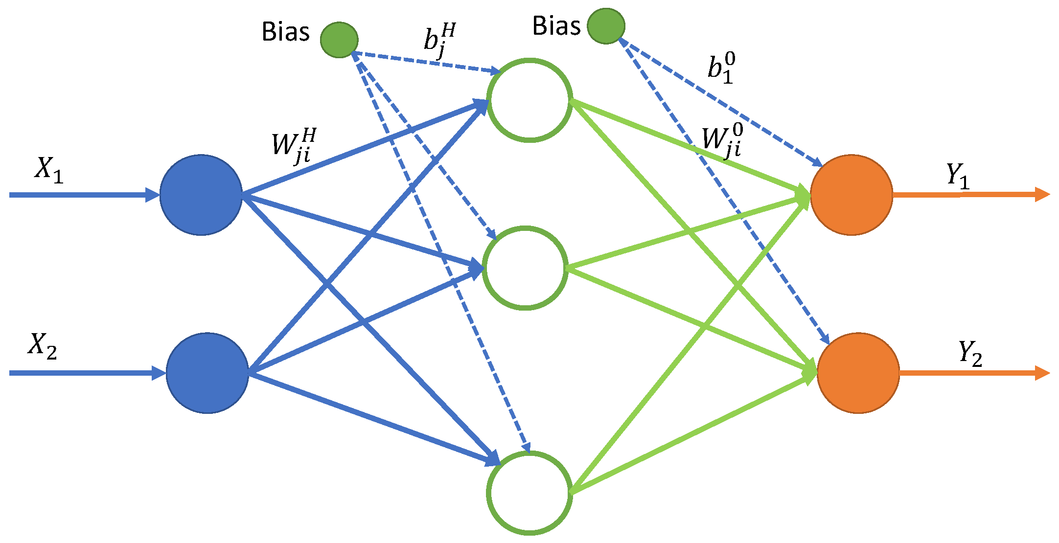
In the MLP, each artificial neuron, receives data from the network input or from other neurons, and produces an output which is a function of the input values and the neuron’s internal training values.

An MLP model with an insufficient or excessive number of neurons in the hidden layer, for the type of problem being solved, is likely to have problems learning. Convergence is difficult and that leads to time-consuming adjustments. Too few neurons cannot retain enough data and there is underfitting. Too many neurons learn the problem instead of generalizing, and there is overfitting of the data. As yet, there is no analytical method by which to determine the right number of neurons in the hidden layer, only practical recommendations based on experience. In general, a rule is to put a hidden layer with a number of neurons that is the average between the input and the output layer. This number is then optimized through trial-and-error experiments [49,50].

Usually, the selection of the training algorithm is dependent on factors such as the organization of the network, the number of hidden layers, weights and biases, learning error rate, etc. Error gradient-based algorithms are common. They work by adjusting the weights in function of the gradient of the error between the output desired and the output obtained. Slow convergence and high dependence on initial parameters, and the tendency to get stuck in local minima are the limitations of gradient-based algorithms [51].

For a given neuron j, each neural input signal $\left(x_k\right)$ is multiplied by their respective corresponding weight values $\left(w_{kj}\right)$, and the resulting products are added to generate a total weight in the form of $w_{j1}{x}_1+w_{j2}{x}_2+\cdots +w_{jm}{x}_m$. The sum of the weighted inputs and the bias Equation (1) forms the input for the activation function, $\phi$. The activation function $\phi$ processes this sum and provides the output, $U_j$ neuron output, according to Equation (2) and Figure 4 [52,53]. We have

$$S_j=\sum _{k=1}^{m_j}{w}_{jk}\times x_{k}j+b_j$$

(1)

$$U_j=\phi \left(S_j\right)=\phi (\sum _{k=1}^{m_j}{w}_{jk}\times x_{k}j+b_j).$$

(2)

The symbol $w_{ji}^H$ denotes the synaptic weight between the neuron leaving the hidden layer and the neuron entering the output layer: the symbol $b_j^H$ denotes the neuron bias in the hidden layer; the superscript O is the output layer. In the figure, the green circles indicate biases, which are constants corresponding to the intersection in the conventional regression model [54].

This type of network can be trained by using many different algorithms. Backpropagation is possibly the most common. Other approaches include resilient backpropagation (RPROP) with or without weight backtracking, described in [55], or the globally convergent version (GRPROP) [56].

MLP neural networks are supported by many popular machine learning frameworks. In the Python sklearn library, they are implemented by MLPClassifier and MLPRegressor functions [57].

In the deep learning framework Tensorflow, the function neuralnet implements a sequential model with dense layers [58].

3.2. Convolutional Neural Networks

This type of neural network is specially adequate to process images. They have outstanding results in object detection. Recently, they have also been used in other fields, especially in combination with other neural networks [59,60,61,62]. The first aplication of a CNN dates back from 1998, by Yann LeCunn. Since then, there have been many contributions in order to make those networks more powerful and faster [63]. The operation of a CNN has the principle of filtering features such as lines, curves, and edges in an image. With each added layer, the filtered features form a more complex image of selected details [64]. This neural network has the ability to process features and objects with good accuracy, depending on the type of architecture applied [65,66,67,68,69]. Therefore, it may also be used to process other types of data, in addition to images.

3.3. Recorrent Neural Networks

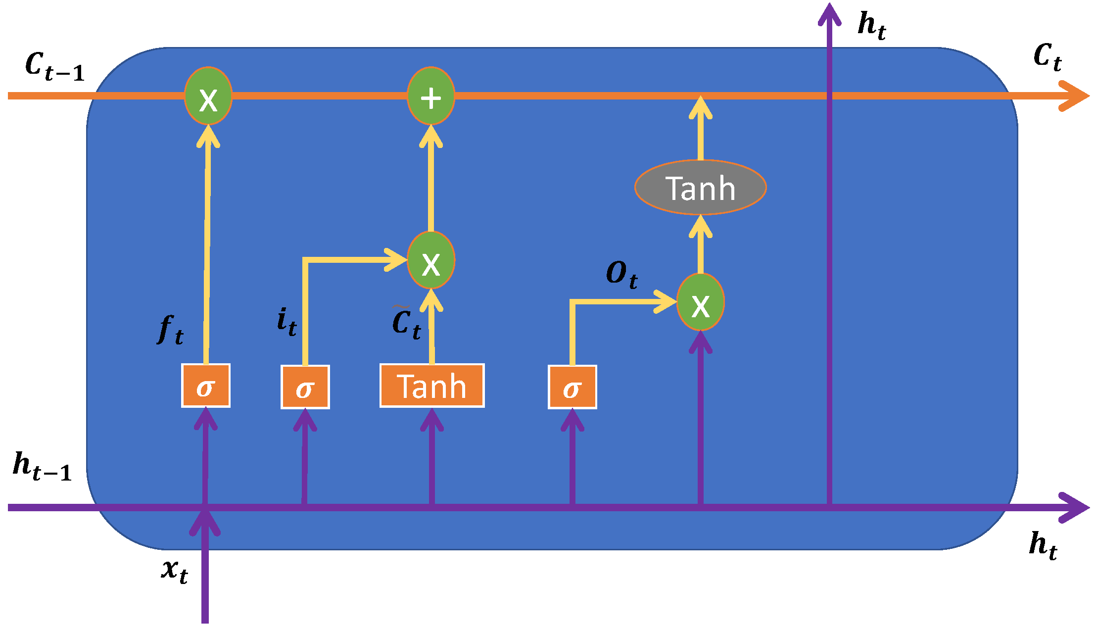
Recurrent, or feedback, networks have their outputs fed back as input signals. This feedback works as a kind of state memory, thus making the networks very suitable to use to process time-varying systems. The signal travels over the network in two directions, having dynamic memory and the ability to represent states in dynamic systems. The present paper particularly focuses on recurrent neural networks known as long short-term memory (LSTM), whose representation is shown in the Figure 5 and gated recurrent unit (GRU).

Hochreiter and Schmidhuber [70] proposed the LSTM cell, which is a popular recurrent model. The LSTM has a capacity to remember, and is controlled by introducing a “gate” into the cell. Since this pioneering work, LSTMs were made popular and used by many researchers [71,72]. According to [73], the internal calculation formula of the LSTM cell is defined as follows:

$$f_t=\sigma (x_t{W}_f+h_{t-1}{U}_f+b_f)$$

(3)

$$i_t=\sigma (x_t{W}_i+h_{t-1}{U}_i+b_i)$$

(4)

$$o_t=\sigma (x_t{W}_o+h_{t-1}{U}_o+b_o)$$

(5)

$${\tilde{\mathit{C}}}_{\mathit{t}}=tan[(x_t{W}_C+h_{t-1}{U}_c+b_c]$$

(6)

$$C_t=\sigma (f_t\times C_{t-1}+i_t\times {\tilde{C}}_t)$$

(7)

$$h_t=tanh\left(C_t\right)\times o_t,$$

(8)

where t is timestep, $x_t$ is input to the current t, $W_f$ is weight associated with the input, $h_{t-1}$ is the hidden state of the previous timestamp, $U_f$ is the weight matrix associated with hidden state, $W_i$ is weight matrix of input, $U_i$ is weight matrix of input associated with hidden state, $C_t$ is memory from current block, and $h_t$ output of current block. The $f_t$ is the forget gate, $i_t$ is input gate, $o_t$ is the output gate, $C_t$ is new cell state, ${\tilde{\mathit{C}}}_{\mathit{t}}$ is values generated by tanh with all the possible values between −1 and 1, and $b_f,b_i,b_o,b_c$ are the bias terms.

Figure 5. Architecture of an LSTM cell; adapted from [73,74,75].

Figure 5. Architecture of an LSTM cell; adapted from [73,74,75].

The learning capacity of the LSTM cell is superior to that of the standard recurrent cell. However, the additional parameters add to the computational load. Cho et al. [76] introduced the gated recurring unit (GRU) model, which is a type of modified version of the LSTM.

Figure 6 shows the internal architecture of a GRU unit cell. These are the mathematical functions used to control the locking mechanism in the GRU cell:

$$z_t=\sigma (x_t{W}^z+h_{t-1}{U}^z+b_z)$$

(9)

$$r_t=\sigma (x_t{W}^r+h_{t-1}{U}^r+b_r)$$

(10)

$${\tilde{\mathit{h}}}_{\mathit{t}}=tan{(x_t{W}_h+(r_t\times h_{t-1})U_h+b)}_h$$

(11)

$$h_t=(1-z_t)\times {\tilde{h}}_t+z_t\times h_{t-1},$$

(12)

where $x_t$ is input vector, $h_t$ is output vector, ${\hat{h}}_t$ is candidate activation vector, $z_t$ is update gate vector, $r_t$ is reset gate vector and, $W^z,W^r,W^h$ denote the weight matrices for the corresponding connected input vector. $U^z,U^r,U$ represent the weight matrices of the previous time step, and $b_r,b_z$, $b_h$ are biases.

3.4. Model Evaluation

For evaluation of the performance of the models, the metrics used are the root mean square error (RMSE) and the mean absolute percentage error (MAPE). RMSE is calculated as in Formula (13) and MAPE is calculated as in Formula (14).

$$\mathrm{R}\mathrm{M}\mathrm{S}\mathrm{E}=\sqrt{\frac{1}{n}\sum _{\begin{array}{c}t=1\end{array}}^n{(Y_t-\hat{Y})}^2}.$$

(13)

$Y_t$ is the actual value, and $\hat{Y}$ is the predicted value obtained from the models. n is the number of samples in the set being evaluated. The RMSE is a type of absolute error, whereas MAPE is an error which is relative to the variable being predicted. The MAPE can only be calculated if the zeros are removed from the dataset. We have

$$\mathrm{M}\mathrm{A}\mathrm{P}\mathrm{E}=\frac{1}{n}\sum _{\begin{array}{c}t=1\end{array}}^n\frac{|Y_t-{\hat{Y}}_t|}{|Y_t|}.$$

(14)

4. Empirical Examination

4.1. Data Analysis

The present study was carried out by using a dataset consisting of samples available on the World Steel website (https://www.worldsteel.org/steel-by-topic/statistics/steel-statistical-yearbook.html (accessed on 7 June 2022 )).

Those samples represent the steel production, per year, in millions of metric tons, in the world, from 1900 to 2021. The values are plotted in Figure 7.

Table 1. Characteristics of the variable annual crude steel production in the world. std is the standard deviation, $Q_1$ is the 25% percentile, $Q_2$ is the 50% percentile, $Q_3$ is the 75% percentile. Max is the maximum value, Min the minimum value and Mean the average value.

Mean	Std	Min.	Max	${\mathit{Q}}_1$	${\mathit{Q}}_2$	${\mathit{Q}}_3$
4.999142 $\times {10}^5$	5.081208 $\times {10}^5$	2.830000 $\times {10}^4$	1.953304 $\times {10}^6$	9.382500 $\times {10}^4$	3.488500 $\times {10}^5$	6.755030 $\times {10}^5$

shows a summary of statistical parameters of the variable. The values show growth over time, as mentioned above, reflecting growth of some sectors such as transport and civil construction. As the chart shows, the production has been small and with a small growth rate in the beginning of the century. After 1945, the growth accelerates, until 1970. Then there is a a period of no growth, followed by a decline and another period of stagnation. After 1995 there is a sharp increase, where the growth accelerated very quickly. The variable is particularly difficult to predict, because the periods described above are clearly distinct.

4.2. Experiments

The experiments performed consist of testing different model architectures and hyperparameters, in order to find the best predictive models. All expriments used the same sequence of actions present in Figure 8.

The data has a sampling rate per year; for all three variables the sample set has a size of 72 samples. In this phase the data were adjusted in order to have the same sample size in the same time period.

The dataset was divided in two parts, one for training and the other for testing. For the first test, the train subset is 70% of the data, the test subset is the remaining 30%. The second test where use the architecture encoder–decoder was used in the train subset is 80% and the test subset is 20%. The training process was allowed to proceed for up to 2000 epochs.

The experiments were performed in order to understand the impact of varying the size of the window of past samples, as well as the the number of years in advance. Naturally, the larger the number of years ahead that is being predicted (gap), the larger the error expected. The larger the size of the historical window used, the smaller the error expected, up to a certain size. As mentioned above, the evolution of the variable has distinct patterns over the years. Therefore, too many samples from the past may carry patterns that are not applicable to the future.

Figure 9 and Figure 10 show a summary of the best results obtained for different neural network models, namely MLP, CNN-MLP, LSTM, CNN-LSTM, GRU, and CNN-GRU. The window size varied between 4 and 16 years. The gap was varied between 1 and 9 years.

Table 2. Predictive models with the best results.

	Model
Architecture	Unit	Activation Function
CNNLSTM	CNN = 64, LSTM = 50	Relu
MLP	MLP = 50	Relu
GRU encoder decoder	GRU = 200	Relu

summarizes the architectures that presented the best performance.

Figure 9 and Figure 10 shows the RMSE and MAPE errors for different window sizes and gaps. As the Figure 11 show, the CNN LSTM and the MLP offers lower errors for wider gaps, even with small windows.

Table 3. Description of the variables steel production, producer price index by commodity, and world population.

	Steel Production	Iron and Steel	World Population
count	7.200000	72.000000	7.200000
mean	7.863977 $\times {10}^5$	107.355084	5.008493 $\times {10}^9$
std	4.856869 $\times {10}^5$	77.016810	1.655973 $\times {10}^9$
min	1.916000 $\times {10}^5$	19.058333	2.499322 $\times {10}^9$
25%	5.038660 $\times {10}^5$	29.931250	3.528970 $\times {10}^9$
50%	6.130825 $\times {10}^5$	104.683333	4.905897 $\times {10}^9$
75%	9.953132 $\times {10}^5$	137.208333	6.414362 $\times {10}^9$
max	1.953304 $\times {10}^6$	356.707750	7.909295 $\times {10}^9$

shows the description of the variables, as they present different magnitudes. Because we do not intend to have this type of problem, we performed the normalization of all variables as shown in Figure 12.

The models performed well for both short- and long-term forecasts. Models with encoder–decoder architecture were also tested in order to improve the steel production forecast results by using the market variables and their derivatives that affect the steel production variable (producer price index by commodity https://fred.stlouisfed.org/series/PPIACO (accessed on 14 June 2022), world population https://www.macrotrends.net/countries/WLD/world/population (accessed on 14 June 2022)) as shown in Figure 12.

As can be seen from Figure 13, the variables have a good correlation. In the case of the derivatives, the correlations are weak, and the derivative that has a reasonable correlation in relation to steel production is the world population.

By using the same architecture with GRU units, we conducted two tests, the first consisting of adding one variable at a time to the model until reaching the six variables with their derivatives. With this, the results of Figure 14 achieved a good prediction of the variable under study with the input of the three variables as is shown in the graph.

The second test had the goal of testing the neural network, having as input two variables in the network. One of them is fixed (steel production) and the other is variable. As can be seen in Figure 15, the variables steel production and world population, or steel production and world population derivative, are the ones that present the best results.

5. Discussion

Artificial intelligence is the field of knowledge concerned with developing techniques that allow computers to act in a way that looks like an intelligent organism.

Table 4. MAPE errors of tests with different historical windows (4–14 samples) and gaps (years ahead) ranging from 1 to 8.

Window	Gap	MLP	LSTM	GRU	CNNMLP	CNNLSTM	CNNGRU
	1	4.54	5.18	4.67	4.75	5.9	5.59
	2	6.93	7.5	7.99	7.29	7.57	6.93
	3	9.84	10.12	9.66	9.0	8.67	9.67
	4	10.77	11.91	11.55	10.82	10.06	10.49
4	5	12.7	13.97	12.76	13.06	11.74	12.09
	6	14.15	15.24	13.44	13.05	13.36	12.84
	7	15.77	16.76	16.24	15.09	14.44	15.74
	8	18.78	18.08	18.23	17.35	15.96	19.54
	1	5.65	4.86	4.85	4.73	5.56	6.89
	2	9.42	8.94	7.71	7.87	9.16	9.12
	3	10.04	10.38	9.17	9.68	10.76	11.18
	4	11.97	11.46	10.49	10.55	9.43	11.49
6	5	12.97	12.5	12.1	10.84	11.27	11.13
	6	14.03	14.17	14.21	14.52	12.23	10.55
	7	15.71	15.82	16.0	14.01	12.42	11.81
	8	17.46	16.81	18.23	16.24	20.43	15.6
	1	5.85	5.11	5.23	4.59	4.85	5.52
	2	8.62	9.54	7.18	6.82	6.21	7.16
	3	10.03	10.29	9.71	10.32	7.3	7.58
	4	11.89	11.06	10.63	11.71	6.71	7.63
8	5	11.62	14.9	12.2	11.26	10.79	8.71
	6	14.37	14.39	13.84	12.03	12.55	15.48
	7	15.46	14.63	15.3	18.41	6.22	9.3
	8	17.88	15.46	17.13	15.17	7.88	6.35
	1	5.61	5.02	5.09	5.46	5.06	5.41
	2	9.74	14.0	7.73	7.03	6.59	7.16
	3	9.66	10.88	9.44	9.96	7.35	8.11
	4	10.67	11.78	12.35	10.19	7.99	11.23
10	5	12.6	14.67	13.81	10.96	12.42	12.07
	6	13.11	13.78	13.58	10.96	9.72	16.83
	7	14.43	15.57	14.47	13.0	16.32	11.52
	8	15.05	16.14	17.25	16.15	8.81	4.82
	1	5.28	7.33	5.74	5.59	5.42	5.66
	2	7.84	10.03	8.77	8.48	5.61	9.4
	3	10.2	11.14	10.36	10.66	9.13	8.96
	4	9.56	13.64	12.02	9.71	11.11	11.14
12	5	9.92	13.13	12.01	11.98	13.51	14.32
	6	11.69	13.66	12.17	10.89	13.35	18.05
	7	17.06	17.13	15.76	12.62	16.6	27.02
	8	14.25	14.22	16.95	18.39	12.83	23.63
	1	5.69	5.71	5.5	6.13	4.31	6.31
	2	8.89	12.5	8.65	7.99	10.84	10.35
	3	11.3	11.88	8.86	9.06	12.64	14.12
	4	11.25	12.83	11.89	9.26	14.58	13.7
14	5	14.51	10.34	12.58	10.59	13.47	15.48
	6	11.35	14.93	9.6	10.02	13.37	13.88
	7	15.73	14.47	12.37	12.4	14.09	15.97
	8	15.77	11.62	13.67	13.47	16.4	30.38

shows a summary of MAPE errors for the models tested, for different gaps (1 to 9 years ahead) and for different historical windows (4–14 samples). The table shows that the models, especially the ones with higher sliding windows and a convolutional layer, present a better MAPE. The convolutional layer contributes to improve convergence during learning.

The table also shows that for all models, the greater the value of the gap, the larger the errors, which is an expected result. In general it is possible to obtain errors of about 5% for the next year, but for an advance of three years and beyond, the errors less than 10% are very rare.

By inputting other variables that have a significant correlation with the steel production variables, it was found that these and their derivatives can have an impact on the predicted values.

The results also show that the size of the historical sliding window is important, but larger windows are not always better than smaller windows. A window of 10 samples offers some of the best results when the convolution layer is used, for the LSTM and GRU models. The convolutional layer seems to offer some stability in the LSTM and GRU models for midterm predictions, when historical windows of 10–12 samples are used.

6. Conclusions

Production management is the process or activity by which resources flow within a defined system, and are grouped and transformed in a controlled manner to add value, according to the policies defined by a company.

As presented in the literature review, steel plays an active role in human activities. Figure 7 shows the amount of steel produced annually around the world. Because steel is a finite and important natural resource, monitoring it is a key strategic issue for companies and others; hence the importance of forecasting so that decisions can be made in advance.

A reliable forecasting method can be a key asset to anticipate good and bad periods, giving the management opportunity to react and take measures in time and possibly avoid losses.

The present paper demonstrates the behavior of different predictive models, particularly the combination of convolutional layers for the MLP, LSTM, and GRU. The results show that each model presents a particularity regarding the delay windows and the advance windows.

Table 4 shows that for the delay window equal to 4 and 12 the MLP model shows better accuracy. For the delay window equal to 6 and 8, it is the CNNMLP model that shows better accuracy. For the delay window equal to 10, it is the LSTM model that shows better accuracy, and for the delay window equal to 14, it is the CNNLSTM model that shows better accuracy.

The results of the encoder–decoder model presented the best result, although it turned out that these results had a great influence on the input variables of the model. The results also show that it is possible to improve the model if information is added that correlates in some way with the variable being predicted. It should also be noted that much of this information is included in the variables’ derivatives, so differencing can greatly reduce prediction errors.

Future work includes experiments to combine other dependent variables, such as GDP growth, to improve predictions, as well as apply the same models to predict the production of other commodities.

References

- Gajdzik, B.; Sroka, W.; Vveinhardt, J. Energy Intensity of Steel Manufactured Utilising EAF Technology as a Function of Investments Made: The Case of the Steel Industry in Poland. Energies 2021, 14, 5152. [Google Scholar] [CrossRef]
- Tang, L.; Liu, J.; Rong, A.; Yang, Z. A review of planning and scheduling systems and methods for integrated steel production. Eur. J. Oper. Res. 2018, 133, 1–20. [Google Scholar] [CrossRef]
- Pei, M.; Petäjäniemi, M.; Regnell, A.; Wijk, O. Toward a Fossil Free Future with HYBRIT: Development of Iron and Steelmaking Technology in Sweden and Finland. Metals 2020, 10, 972. [Google Scholar] [CrossRef]
- Liu, W.; Zuo, H.; Wang, J.; Xue, Q.; Ren, B.; Yang, F. The production and application of hydrogen in steel industry. Int. J. Hydrogen Energy 2021, 46, 10548–10569. [Google Scholar] [CrossRef]
- Eisenhardt, K.M. Strategy as strategic decision making. MIT Sloan Manag. Rev. 1999, 40, 65. [Google Scholar]
- Anderson, K. The Political Market for Government Assistance to Australian Manufacturing Industries. In World Scientific Reference on Asia-Pacific Trade Policies; World Scientific: Singapore, 2018; pp. 545–567. [Google Scholar] [CrossRef]
- Redclift, M. Sustainable Development: Exploring the Contradictions; Routledge: London, UK, 1987. [Google Scholar] [CrossRef] [Green Version]
- Holmberg, J.; Sandbrook, R. Sustainable Development: What Is to Be Done? In Policies for a Small Planet; Routledge: London, UK, 1992; 20p. [Google Scholar]
- Colla, V.; Branca, T.A. Sustainable Steel Industry: Energy and Resource Efficiency, Low-Emissions and Carbon-Lean Production. Metals 2021, 11, 1469. [Google Scholar] [CrossRef]
- Rodrigues, J.; Cost, I.; Farinha, J.T.; Mendes, M.; Margalho, L. Predicting motor oil condition using artificial neural networks and principal component analysis. Eksploat. Niezawodn.-Maint. Reliab. 2020, 22, 440–448. [Google Scholar] [CrossRef]
- Iruela, J.R.S.; Ruiz, L.G.B.; Capel, M.I.; Pegalajar, M.C. A TensorFlow Approach to Data Analysis for Time Series Forecasting in the Energy-Efficiency Realm. Energies 2021, 14, 4038. [Google Scholar] [CrossRef]
- Ramos, D.; Faria, P.; Vale, Z.; Mourinho, J.; Correia, R. Industrial Facility Electricity Consumption Forecast Using Artificial Neural Networks and Incremental Learning. Energies 2020, 13, 4774. [Google Scholar] [CrossRef]
- Coccia, M. Steel market and global trends of leading geo-economic players. Int. J. Trade Glob. Mark. 2014, 7, 36. [Google Scholar] [CrossRef]
- Sala, D.A.; Yperen-De Deyne, V.; Mannens, E.; Jalalvand, A. Hybrid static-sensory data modeling for prediction tasks in basic oxygen furnace process. Appl. Intell. 2022. [Google Scholar] [CrossRef]
- Chen, C.J.; Chou, F.I.; Chou, J.H. Temperature Prediction for Reheating Furnace by Gated Recurrent Unit Approach. IEEE Access 2022, 10, 33362–33369. [Google Scholar] [CrossRef]
- Janka, D.; Lenders, F.; Wang, S.; Cohen, A.; Li, N. Detecting and locating patterns in time series using machine learning. Control Eng. Pract. 2019, 93, 104169. [Google Scholar] [CrossRef]
- Kim, K.; Seo, B.; Rhee, S.H.; Lee, S.; Woo, S.S. Deep Learning for Blast Furnaces: Skip-Dense Layers Deep Learning Model to Predict the Remaining Time to Close Tap-Holes for Blast Furnaces. In Proceedings of the 28th ACM International Conference on Information and Knowledge Management, CIKM ’19, Beijing, China, 3–7 November 2019; Association for Computing Machinery: New York, NY, USA, 2019; pp. 2733–2741. [Google Scholar] [CrossRef] [Green Version]
- Xuan, Y.; Yue, Q. Forecast of steel demand and the availability of depreciated steel scrap in China. Resour. Conserv. Recycl. 2016, 109, 1–12. [Google Scholar] [CrossRef]
- Crompton, P. Future trends in Japanese steel consumption. Resour. Policy 2000, 26, 103–114. [Google Scholar] [CrossRef]
- Gajdzik, B. Steel production in Poland with pessimistic forecasts in COVID-19 crisis. Metalurgija 2021, 60, 169–172. [Google Scholar]
- Wang, P.; Jiang, Z.-Y.; Zhang, X.-X.; Geng, X.-Y.; Hao, S.-Y. Long-term scenario forecast of production routes, energy consumption and emissions for Chinese steel industry. Chin. J. Eng. 2014, 36, 1683–1693. [Google Scholar] [CrossRef]
- Sharma, A.; Kumar, S.; Duriagina, Z. Engineering Steels and High Entropy-Alloys, 1st ed.; BoD—Books on Demand: London, UK, 2020. [Google Scholar]
- Javaid, A.; Essadiqi, E. Final report on scrap management, sorting and classification of steel. Gov. Can. 2003, 23, 1–22. [Google Scholar]
- Carilier, M. Distribution of Steel END-Usage Worldwide in 2019, by Sector. 2021. Available online: https://www.statista.com/statistics/1107721/steel-usage-global-segment/ (accessed on 2 February 2022).
- Worldsteel|Global Crude Steel Output Decreases by 0.9% in 2020. 2021. Available online: http://www.worldsteel.org/media-centre/press-releases/2021/Global-crude-steel-output-decreases-by-0.9--in-2020.html (accessed on 2 February 2022).
- Moya, J.A.; Pardo, N. The potential for improvements in energy efficiency and CO2 emissions in the EU27 iron and steel industry under different payback periods. J. Clean. Prod. 2013, 52, 71–83. [Google Scholar] [CrossRef]
- Crompton, P. Explaining variation in steel consumption in the OECD. Resour. Policy 2015, 45, 239–246. [Google Scholar] [CrossRef]
- Yin, X.; Chen, W. Trends and development of steel demand in China: A bottom–up analysis. Resour. Policy 2013, 38, 407–415. [Google Scholar] [CrossRef]
- Mohr, S.H.; Evans, G.M. Forecasting coal production until 2100. Fuel 2009, 88, 2059–2067. [Google Scholar] [CrossRef] [Green Version]
- Berk, I.; Ediger, V.S. Forecasting the coal production: Hubbert curve application on Turkey’s lignite fields. Resour. Policy 2016, 50, 193–203. [Google Scholar] [CrossRef]
- Mengshu, S.; Yuansheng, H.; Xiaofeng, X.; Dunnan, L. China’s coal consumption forecasting using adaptive differential evolution algorithm and support vector machine. Resour. Policy 2021, 74, 102287. [Google Scholar] [CrossRef]
- Raynor, W.J. The International Dictionary of Artificial Intelligence, Library ed.; Glenlake Pub. Co.; Fitzroy Dearborn Pub: Chicago, IL, USA, 1999; Volume 1, OCLC: Ocm43433564. [Google Scholar]
- Cirstea, M.; Dinu, A.; McCormick, M.; Khor, J.G. Neural and Fuzzy Logic Control of Drives and Power Systems; Google-Books-ID: pXVgBWRMdgQC; Elsevier: Amsterdam, The Netherlands, 2002. [Google Scholar]
- Mateus, B.C.; Mendes, M.; Farinha, J.T.; Cardoso, A.J.M. Anticipating Future Behavior of an Industrial Press Using LSTM Networks. Appl. Sci. 2021, 11, 6101. [Google Scholar] [CrossRef]
- Gubbi, J.; Buyya, R.; Marusic, S.; Palaniswami, M. Internet of Things ({IoT}): A vision, architectural elements, and future directions. Future Gener. Comput. Syst. 2013, 29, 1645–1660. [Google Scholar] [CrossRef] [Green Version]
- Vaio, A.D.; Hassan, R.; Alavoine, C. Data intelligence and analytics: A bibliometric analysis of human–Artificial intelligence in public sector decision-making effectiveness. Technol. Forecast. Soc. Chang. 2022, 174, 121201. [Google Scholar] [CrossRef]
- Niu, Y.; Ying, L.; Yang, J.; Bao, M.; Sivaparthipan, C.B. Organizational business intelligence and decision making using big data analytics. Inf. Process. Manag. 2021, 58, 102725. [Google Scholar] [CrossRef]
- Chen, J.; Gusikhin, O.; Finkenstaedt, W.; Liu, Y.N. Maintenance, Repair, and Operations Parts Inventory Management in the Era of Industry 4.0. IFAC-PapersOnLine 2019, 52, 171–176. [Google Scholar] [CrossRef]
- Farinha, J.M.T. Asset Maintenance Engineering Methodologies, 1st ed.; Taylor & Francis Ltd.: Abingdon, UK, 2018. [Google Scholar]
- Asri, H. Big Data and IoT for real-time miscarriage prediction A clustering comparative study. Procedia Comput. Sci. 2021, 191, 200–206. [Google Scholar] [CrossRef]
- Soltanali, H.; Khojastehpour, M.; Farinha, J.T.; Pais, J.E.d.A.e. An Integrated Fuzzy Fault Tree Model with Bayesian Network-Based Maintenance Optimization of Complex Equipment in Automotive Manufacturing. Energies 2021, 14, 7758. [Google Scholar] [CrossRef]
- Martins, A.; Fonseca, I.; Farinha, J.T.; Reis, J.; Cardoso, A.J.M. Maintenance Prediction through Sensing Using Hidden Markov Models—A Case Study. Appl. Sci. 2021, 11, 7685. [Google Scholar] [CrossRef]
- Sidhu, T.S.; Singh, H.; Sachdev, M.S. Design, implementation and testing of an artificial neural network based fault direction discriminator for protecting transmission lines. IEEE Trans. Power Deliv. 1995, 10, 697–706. [Google Scholar] [CrossRef]
- Das, R.; Kunsman, S.A. A novel approach for ground fault detection. In Proceedings of the 57th Annual Conference for Protective Relay Engineers, College Station, TX, USA, 1 April 2004; pp. 97–109. [Google Scholar] [CrossRef]
- Lippmann, R. An introduction to computing with neural nets. Expert Syst. Appl. 1987, 4, 4–22. [Google Scholar] [CrossRef]
- Orhan, U.; Hekim, M.; Ozer, M. EEG signals classification using the K-means clustering and a multilayer perceptron neural network model. Expert Syst. Appl. 2011, 38, 13475–13481. [Google Scholar] [CrossRef]
- Lee, S.; Choeh, J.Y. Predicting the helpfulness of online reviews using multilayer perceptron neural networks. Expert Syst. Appl. 2014, 41, 3041–3046. [Google Scholar] [CrossRef]
- Ferasso, M.; Alnoor, A. Artificial Neural Network and Structural Equation Modeling in the Future. In Artificial Neural Networks and Structural Equation Modeling; Springer: Berlin/Heidelberg, Germany, 2022; pp. 327–341. [Google Scholar] [CrossRef]
- Hazarika, N.; Chen, J.Z.; Tsoi, A.; Sergejew, A. Classification of EEG signals using the wavelet transform. Signal Process 1997, 59, 61–72. [Google Scholar] [CrossRef]
- Oğulata, S.N.; Şahin, C.; Erol, R. Neural network-based computer-aided diagnosis in classification of primary generalized epilepsy by EEG signals. J. Med. Syst. 2009, 33, 107–112. [Google Scholar] [CrossRef]
- Faris, H.; Aljarah, I.; Al-Madi, N.; Mirjalili, S. Optimizing the Learning Process of Feedforward Neural Networks Using Lightning Search Algorithm. Int. J. Artif. Intell. Tools 2016, 25, 1650033. [Google Scholar] [CrossRef]
- Bonilla Cardona, D.A.; Nedjah, N.; Mourelle, L.M. Online phoneme recognition using multi-layer perceptron networks combined with recurrent non-linear autoregressive neural networks with exogenous inputs. Neurocomputing 2017, 265, 78–90. [Google Scholar] [CrossRef]
- Ding, H.; Dong, W. Chaotic feature analysis and forecasting of Liujiang River runoff. Soft Comput. 2016, 20, 2595–2609. [Google Scholar] [CrossRef]
- Zhang, Z. Neural networks: Further insights into error function, generalized weights and others. Ann. Transl. Med. 2016, 4, 300. [Google Scholar] [CrossRef] [PubMed] [Green Version]
- Riedmiller, M.; Braun, H. A direct adaptive method for faster backpropagation learning: The RPROP algorithm. In Proceedings of the IEEE International Conference on Neural Networks, San Francisco, CA, USA, 28 March–1 April 1993; Volume 1, pp. 586–591. [Google Scholar] [CrossRef]
- Anastasiadis, A.D.; Magoulas, G.D.; Vrahatis, M.N. New globally convergent training scheme based on the resilient propagation algorithm. Neurocomputing 2005, 64, 253–270. [Google Scholar] [CrossRef]
- Pedregosa, F.; Varoquaux, G.; Gramfort, A.; Michel, V.; Thirion, B.; Grisel, O.; Blondel, M.; Prettenhofer, P.; Weiss, R.; Dubourg, V.; et al. Scikit-learn: Machine Learning in Python. J. Mach. Learn. Res. 2011, 12, 2825–2830. [Google Scholar]
- Abadi, M.; Agarwal, A.; Barham, P.; Brevdo, E.; Chen, Z.; Citro, C.; Corrado, G.S.; Davis, A.; Dean, J.; Devin, M.; et al. TensorFlow: Large-Scale Machine Learning on Heterogeneous Systems. 2015. Available online: tensorflow.org (accessed on 4 May 2022).
- Badawi, A.A.; Chao, J.; Lin, J.; Mun, C.F.; Sim, J.J.; Tan, B.H.M.; Nan, X.; Aung, K.M.M.; Chandrasekhar, V.R. Towards the AlexNet Moment for Homomorphic Encryption: HCNN, theFirst Homomorphic CNN on Encrypted Data with GPUs. arXiv 2020, arXiv:1811.00778. [Google Scholar] [CrossRef]
- Arya, S.; Singh, R. A Comparative Study of CNN and AlexNet for Detection of Disease in Potato and Mango leaf. In Proceedings of the 2019 International Conference on Issues and Challenges in Intelligent Computing Techniques (ICICT), Ghaziabad, India, 27–28 September 2019; Volume 1, pp. 1–6. [Google Scholar] [CrossRef]
- Zou, M.; Zhu, S.; Gu, J.; Korunovic, L.M.; Djokic, S.Z. Heating and Lighting Load Disaggregation Using Frequency Components and Convolutional Bidirectional Long Short-Term Memory Method. Energies 2021, 14, 4831. [Google Scholar] [CrossRef]
- Seo, D.; Huh, T.; Kim, M.; Hwang, J.; Jung, D. Prediction of Air Pressure Change Inside the Chamber of an Oscillating Water Column–Wave Energy Converter Using Machine-Learning in Big Data Platform. Energies 2021, 14, 2982. [Google Scholar] [CrossRef]
- Zhu, F.; Ye, F.; Fu, Y.; Liu, Q.; Shen, B. Electrocardiogram generation with a bidirectional LSTM-CNN generative adversarial network. Sci. Rep. 2019, 9, 6734. [Google Scholar] [CrossRef] [Green Version]
- Bouzerdoum, M.; Mellit, A.; Massi Pavan, A. A hybrid model (SARIMA–SVM) for short-term power forecasting of a small-scale grid-connected photovoltaic plant. Sol. Energy 2013, 98, 226–235. [Google Scholar] [CrossRef]
- Zheng, L.; Xue, W.; Chen, F.; Guo, P.; Chen, J.; Chen, B.; Gao, H. A Fault Prediction Of Equipment Based On CNN-LSTM Network. In Proceedings of the 2019 IEEE International Conference on Energy Internet (ICEI), Nanjing, China, 27–31 May 2019. [Google Scholar] [CrossRef]
- Pan, S.; Wang, J.; Zhou, W. Prediction on Production of Oil Well with Attention-CNN-LSTM; IOP Publishing: Bristol, UK, 2021; Volume 2030, p. 012038. [Google Scholar] [CrossRef]
- Li, X.; Yi, X.; Liu, Z.; Liu, H.; Chen, T.; Niu, G.; Yan, B.; Chen, C.; Huang, M.; Ying, G. Application of novel hybrid deep leaning model for cleaner production in a paper industrial wastewater treatment system. J. Clean. Prod. 2021, 294, 126343. [Google Scholar] [CrossRef]
- He, Y.; Liu, Y.; Shao, S.; Zhao, X.; Liu, G.; Kong, X.; Liu, L. Application of CNN-LSTM in Gradual Changing Fault Diagnosis of Rod Pumping System. Math. Probl. Eng. 2019, 2019, 4203821. [Google Scholar] [CrossRef]
- Ren, L.; Dong, J.; Wang, X.; Meng, Z.; Zhao, L.; Deen, M.J. A Data-Driven Auto-CNN-LSTM Prediction Model for Lithium-Ion Battery Remaining Useful Life. IEEE Trans. Ind. Inform. 2021, 17, 3478–3487. [Google Scholar] [CrossRef]
- Hochreiter, S.; Schmidhuber, J. Long Short-Term Memory. Neural Comput. 1997, 9, 1735–1780. [Google Scholar] [CrossRef] [PubMed]
- Rodrigues, J.; Farinha, J.; Mendes, M.; Mateus, R.; Cardoso, A. Comparison of Different Features and Neural Networks for Predicting Industrial Paper Press Condition. Energies 2022, 15, 6308. [Google Scholar] [CrossRef]
- Gers, F.A.; Schmidhuber, E. LSTM recurrent networks learn simple context-free and context-sensitive languages. IEEE Trans. Neural Netw. 2001, 12, 1333–1340. [Google Scholar] [CrossRef] [PubMed]
- Yu, Y.; Si, X.; Hu, C.; Zhang, J. A review of recurrent neural networks: LSTM cells and network architectures. Neural Comput. 2019, 31, 1235–1270. Available online: https://direct.mit.edu/neco/article-pdf/31/7/1235/1053200/neco_a_01199.pdf (accessed on 4 May 2022). [CrossRef] [PubMed]
- Mateus, B.C.; Mendes, M.; Farinha, J.T.; Assis, R.; Cardoso, A.J.M. Comparing LSTM and GRU Models to Predict the Condition of a Pulp Paper Press. Energies 2021, 14, 6958. [Google Scholar] [CrossRef]
- Costa Silva, D.F.; Galvão Filho, A.R.; Carvalho, R.V.; de Souza, L.; Ribeiro, F.; Coelho, C.J. Water Flow Forecasting Based on River Tributaries Using Long Short-Term Memory Ensemble Model. Energies 2021, 14, 7707. [Google Scholar] [CrossRef]
- Cho, K.; van Merrienboer, B.; Bahdanau, D.; Bengio, Y. On the Properties of Neural Machine Translation: Encoder-Decoder Approaches. arXiv 2014, arXiv:1409.1259. [Google Scholar]
- Li, P.; Luo, A.; Liu, J.; Wang, Y.; Zhu, J.; Deng, Y.; Zhang, J. Bidirectional Gated Recurrent Unit Neural Network for Chinese Address Element Segmentation. ISPRS Int. J. Geo-Inf. 2020, 9, 635. [Google Scholar] [CrossRef]
Figure 1.
Results of the searches in the scientific articles databases.
Figure 2.
Annual crude steel production, per industrial consumer sector; Graph created from data taken from source [
24].
Figure 3.
Annual crude steel production for 2019 and 2020; adapted from [
25].
Figure 4.
Representation of a multilayer perceptron, with input X, one hidden layer, and output Y.
Figure 6.
Architecture of a GRU unit; adapted from [
76,
77].
Figure 7.
Annual crude steel production in the world, in millions of metric tons.
Figure 8.
Procedure used to train and test the models to predict steel production in the world.
Figure 9.
RMSE and MAPE for different historical window sizes (number of past samples) and gaps (years ahead), from CNNLSTM model.
Figure 10.
RMSE and MAPE for different windows (number of past samples) and gaps (number of years ahead) from the MLP model.
Figure 11.
Predictions of the best forecast models based on CNNLSTM and MLP models, with and without the convolutional layer. The blue line is the actual value. The orange line is the prediction based on the training set, and the gray line is the prediction based on the test set. The predictions were obtained with window width 4 and gap 1.
Figure 12.
Steel production, producer price index by commodity, and world population in format time series.
Figure 13.
Correlation of the variables steel production, producer price index by commodity, world population, and their first derivates in time series.
Figure 14.
The test error one, used the same architecture with GRU unit.
Figure 15.
The test error two, used the same architecture with GRU unit.