1. Introduction
Image processing has become more and more important in many fields, such as machine vision, geological prospecting, medical imaging, defect detection, and so on. In the past decades, many methods have been presented based on different views, and nonlinear diffusion is one of the most important techniques for the solid mathematical physics foundation [
1,
2,
3]. Different from the uniform diffusion (holds the same velocity along any direction), nonlinear diffusion can be applied to describe lots of complex natural phenomenons. Nonlinear diffusion models are often driven by partial differential equations (PDEs) which can be derived by minimizing an energy functional and computing the Euler–Lagrange equation [
4,
5].
Perona and Malik (PM) proposed a nonlinear diffusion model with a fixed edge stop velocity function related to the local gradient mode [
6]. It can be applied to achieve some denoising tasks with homogeneous features and noise; however, it is difficult to efficiently govern the diffusion process for some more complex cases. Rudin, Osher and Fatemi (ROF) proposed the classical total variation model to recover noisy images by minimizing a geometric energy functional [
1]. The diffusion can be performed only along the edge to preserve the image features and remove the noise.
Though these traditional methods have been reported to work well in many cases, they are still found to show some unfavorable phenomena, such as the staircase effect, loss of texture features, and so on [
7,
8]. Especially in many industrial scenes, the lighting condition is limited, inhomogeneous and easy to be disturbed so that the observed images are often low-contrast, have an inhomogeneous background and are serious polluted. It is often not a good idea to directly apply the traditional models to these degraded images for defect detection since the mentioned unfavorable effects often become worse in such situations.
Defects detection is often implemented on the images captured by some vision devices, which are effected by some objective factors, such as noise level, brightness, background gray distribution, size and shape of the defects. Lots of efforts have been made to present novel models or algorithms based on different starting points and proper assumptions. Saitoh [
9] presented a machine vision scheme for the inspection of brightness unevenness in LCD panel surfaces. An edge detection algorithm and a genetic algorithm were used to identify discontinuous points and extract the boundary of anomalous brightness region, respectively. Kim et al. [
10] presented an adaptive multiple-level threshold method based on the statistical characteristics of the local area to segment spot-type defects from the background surface. Ng revised the Otsu method for selecting optimal threshold values for both unimodal and bimodal distributions and tested the performance on common defect detection applications [
11]. Krummenacher proposed two machine learning methods to automatically detect the wheel defects, which automatically learn different types of wheel defects and predict during normal operation if a wheel has a defect or not [
12].
In recent years, with different views or assumptions, several improved nonlinear diffusion models were presented for different tasks about image processing and defect detection. Tsai and Chao took a non-negative decreasing function with an annealing gradient threshold as the diffusion coefficient, and then proposed a novel anisotropic diffusion model (TCAD) to detect subtle defects embedded in inhomogeneous textures [
13]. Chao and Tsai introduced a weighted diffusion function and a generalized diffusion coefficient function respectively to the classical PM model for defect detection in low-contrast surface images [
14,
15]. These two models both carry out a smoothing process for faultless areas and perform a sharpening process for defect areas. Based on the directional Laplacian, Wang et al. proposed a modified version (MPM) of the original Perona–Malik model [
16]. A weighted Laplacian was incorporated in the PM model to perform the diffusion along the edge direction of the original image. Prasath and Vorotnikov proposed a weighted and balanced anisotropic diffusion scheme for image denoising and restoration [
17]. Maiseli and Gao presented a robust edge detector based on an anisotropic diffusion-driven process [
18]. In this model, noise suppression and edge enhancement are achieved respectively by anisotropic diffusion and the edge-sensitive detector.
Xu et al. [
19] contributed a new filter by introducing a semi-adaptive threshold to an anisotropic diffusion process. In detail, a Gaussian filter is applied to recognize corrupted pixels in noise-free pixels and then a semi-adaptive threshold function is introduced to the diffusion coefficient for noise removal and edge preservation. Malarvela et al. found that the local probability value of image gray can be applied to adjust the indication degree of a low edge gradient in the feature space of a noisy image, similar to the action of an adaptive threshold parameter [
20]. They proposed an improved anisotropic diffusion model which can adaptively adjust the implication of the image edge gradient in the diffusion process. More research studies about defect detection and image denoising related to other techniques refer to some recent papers [
21,
22,
23,
24,
25].
Based on the above, it can be found most research focuses on designing novel diffusion patterns or using the observed information in new schemes. However, in complex scenes, inconsistent background and features should be properly treated for efficient defect detection. The gradient, Laplacian and some other geometric metrics are often used to describe the observed image features, and they are easily disturbed by an uneven background. In this paper, a novel hybrid energy based on L1 and L2 is introduced to a constrained optimization problem. Then the corresponding Euler–Lagrange equations are derived to form a nonlinear diffusion with a smoothed background estimation, which can remove the noise and preserve more details of the defect features.
This paper is organized as follows. In
Section 2, the basic fundamentals of defect detection and nonlinear diffusion are introduced. Then the proposed model based on a novel hybrid functional is introduced in
Section 3; the algorithm and numerical scheme are also presented.
Section 4 shows the experiments and results.
2. Basis and Fundamentals
Image degradation is a common situation in transmitting image information and recording digital images, but in many practical applications, high-quality images are necessary, so effective methods to improve and recover degraded images are worthy of our study. In this section, we will briefly describe some important image denoising models based on partial differential equations and anisotropic diffusion.
2.1. Nonlinear Diffusion
Perona and Malik proposed a classical nonlinear diffusion model based on the linear diffusion (or heat equation) [
6], and the diffusion process can be represented by a partial differential equation:
where
refers to the image at time
t, div means the divergence operator,
means the spatial gradient of the image at time
t, and
k denotes a threshold linked to the features strength. This partial differential equation can be derived by minimizing a related energy functional:
Here means a diffusion velocity, and it can be replaced by other function as necessary.
In the PM model, the diffusion velocity is determined by a fixed pattern at each iteration, which reduces the diffusion as the gradient module increases to protect the edges present in the image. Some degraded images can be successfully recovered by solving the above equation with a proper initial condition and boundary condition, even if the artifacts still occur in the result due to the instability of the diffusion process.
The total variation model (TV) is another representative one of nonlinear diffusion models, and it was first proposed by Rudin, Osher and Fatami [
1]. The bounded variation (BV) function is introduced to denote the ideal image and then the discontinuities edge can be well-preserved when removing the noise. This model has been widely applied to many other fields as a regularization technique [
26]. It can be denoted as
Here,
f denotes the observed degraded image and
is a Lagrangian multiplier which balances different terms. It can be obtained by minimizing a combined energy functional
Differing from the diffusion controlling mechanism of the PM model, the TV model prevents smoothing across the edge everywhere, even if in an almost plain area. For preserving the discontinuous edge and smoothing the approximately flat area, it is often necessary to carefully design numerical schemes with a small time step.
Based on the TV model and the PM model, lots of research has been presented to improve the results at different views [
3,
27,
28,
29]. The CTAD model [
30] was presented to treat the restoration tasks on astronomical images. The local variance of the image gray is embedded in the diffusion velocity of the model for an adaptive process. Specifically, the advanced diffusion velocity is denoted as
where
is the local variance of gray levels in a proper neighborhood.
A weighted Laplacian was incorporated the modified Perona–Malik model, where the directional Laplacian diffuses the image along the edge direction of the original image [
16]. In this model, the diffusion is designed along a unit directional vector
, and the noise can be suppressed by the weighted Laplace operator. The related partial differential equation can be denoted as
where
,
denotes a small positive constant and
f is the observed degraded image.
Malarvel et al. proposed a modified model that introduces both a probability value and gradient of local image gray to reduce the noise and smooth the noise-free part adaptively [
20]. Thee diffusion velocity can be denoted as
Here parameter k should be a positive fixed constant, and it is related to the strength to denoise and enhance the edge. The input variable p is related to the local gray distribution, and it can be calculated based on image I.
In this paper, we will first introduce several fields related to smoothed estimation and edge information, and then present a novel dynamic mechanism based on them to better determine the diffusion velocity for improvements of the denoising results.
2.2. Some Evaluation Metrics
To measure the qualities of image processing results, some metrics are often applied to calculate the evaluation values. The general evaluation metrics include but are not limited to mean square error (MSE), peak signal-to-noise ratio (PSNR), entropy (ET) and structural similarity (SSIM).
The dissimilarity between the referenced image
and the result image
can be measured by MSE, which means the loss of image quality. Assume that the image size is
, MSE can be calculated as
The PSNR can be defined as
Here, L means the gray level. The lower the MSE, the lesser the error, and MSE is inversely proportional to PSNR.
The entropy is a measure widely applied in many fields such as data mining and image processing. A lesser entropy value implies lesser disorder. The common Shannon entropy (
10) can be used to evaluate the disorder degree or variance of a result image:
Here, means the gray ratio on the ith bin of the normalized image histogram.
SSIM measures the image quality by computing the similarity between the result image and reference image. The SSIM value is limited in
and a larger value indicates that the result image is more similar to the original one.
where
and
represent the average pixels of the two images,
and
represent the standard variance of
I and
u,
is the covariance, and constant
.
3. The Proposed Method
In many complex scenes, image will suffer from inconsistent noise and varying lighting condition, which leads to a nonuniform background. Traditional models can often successfully treat the consistent degradation and uniform background (no or little change in each parts) while being deficient for inconsistent cases. For example, the noise strength is very different in some parts of the image area, the edge consists of some strong parts and some weak parts, and the background gray of some parts are at different levels (inconsistent background). Here, we focus on the image degraded by Gaussian white noise and an inconsistent background.
In this paper, a background gray surface is introduced to the observation model for complex scenes, and then a novel functional based on the combination of L1 and L2 energy is presented to modify the traditional total variation energy. Then, novel nonlinear diffusion equations can be derived to remove the noise and separate the inconsistent background by minimizing the energy functional.
3.1. A Novel Energy Functional
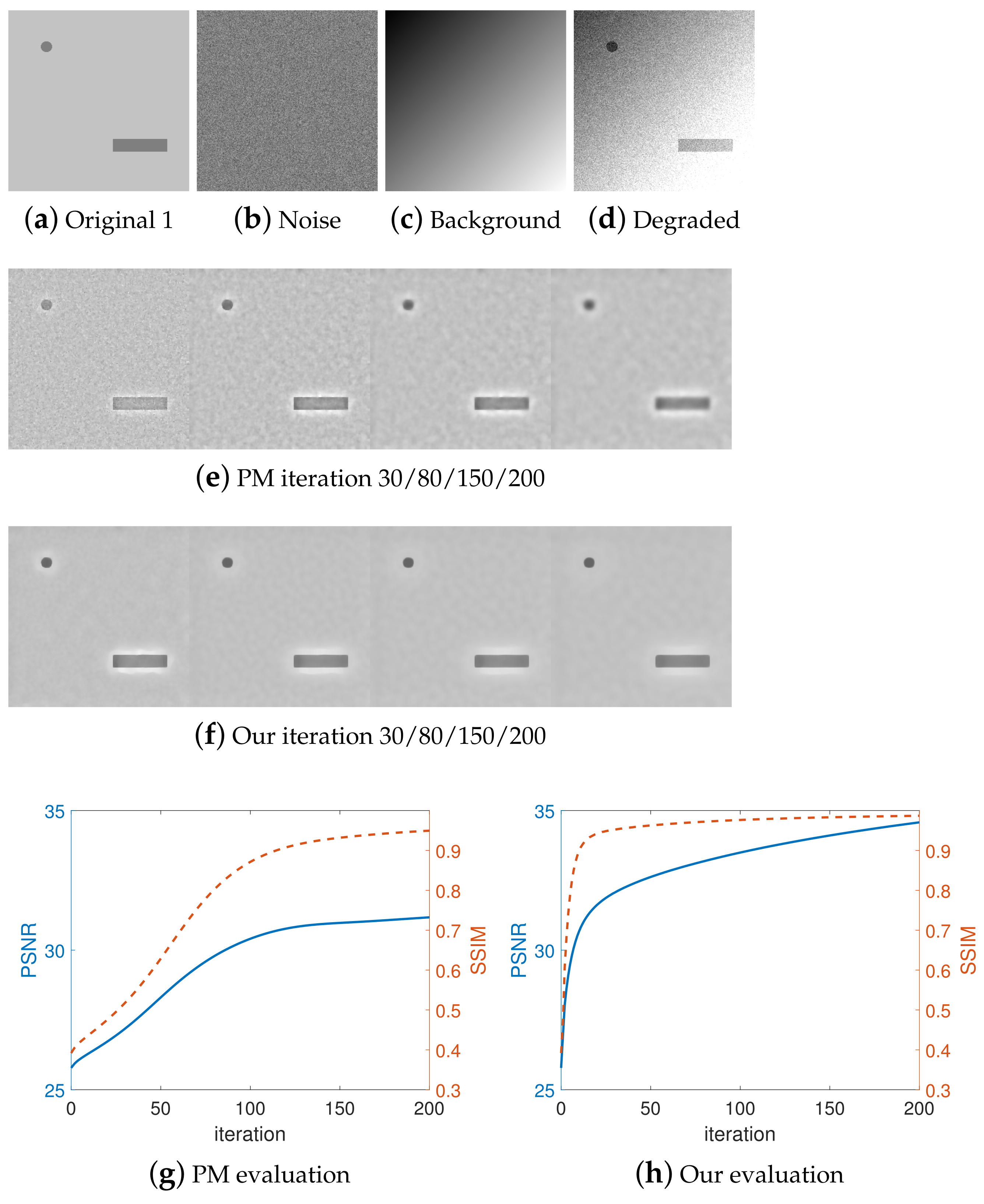
The existence of an inconsistent background (which different in parts) is disadvantageous for treating the polluted and low-contrast image. More exactly, many geometric terms (such as gradient, Laplacian, etc.) are unavoidable to be polluted by not only noise, but also the inconsistent background. Accurate estimation of the background can help to remove the noise and enhance the image quality more efficiently. The observation can be generally denoted as
, and a simple example is shown in the first row of
Figure 1. Here,
f is the observed image polluted by Gaussian white noise
n with variance
and inconsistent background
v, and
I is the clear version of
f. Assume that
v is almost smooth everywhere, then a novel energy functional is presented as
It can be found that the first term means the total variation of the ideal image I. The second term is the energy of the gradient field of background v and the minimization can be linked to solve a smoothing version of v. The third term is the total variation of , and the minimization means an edge-preserved process. and are both weight factors to balance these terms.
Based on the observation model, the variance prior of the noise can be related to a fitting functional
. In a dynamic minimization process, it can limit the solved
not far away from the observation
f. Then an optimization problem to determine
can be denoted as
Apply the Lagrange method and then the above problem is equivalent to an unconstrained optimization problem, that is
Here,
means a Lagrange multiplier to combine the geometric energy and the fitting error. Apply the following Euler–Lagrange equations to compute the gradient flow of (
13), and introduce the artificial term
, the final evolution equations can be obtained as (
14)
In the evolution, the first equation will preserve the features, including defects to be detected due to the two total variation diffusion terms. The second equation is mainly to approximate the ideal background v while features are well-protected.
Set the homogeneous Neumann boundary condition on
, that is
where
means the normal vector on the boundary
. Set the initial condition in
then Equation (
14) can be solved by some numerical methods, such as finite difference.
Here,
means an initial estimation of the background.
Figure 1 shows the traditional evolution and the proposed evolution on an artificial image with two suspect areas. The first row shows the original image, the noise, the inconsistent background and the degraded image. As shown in
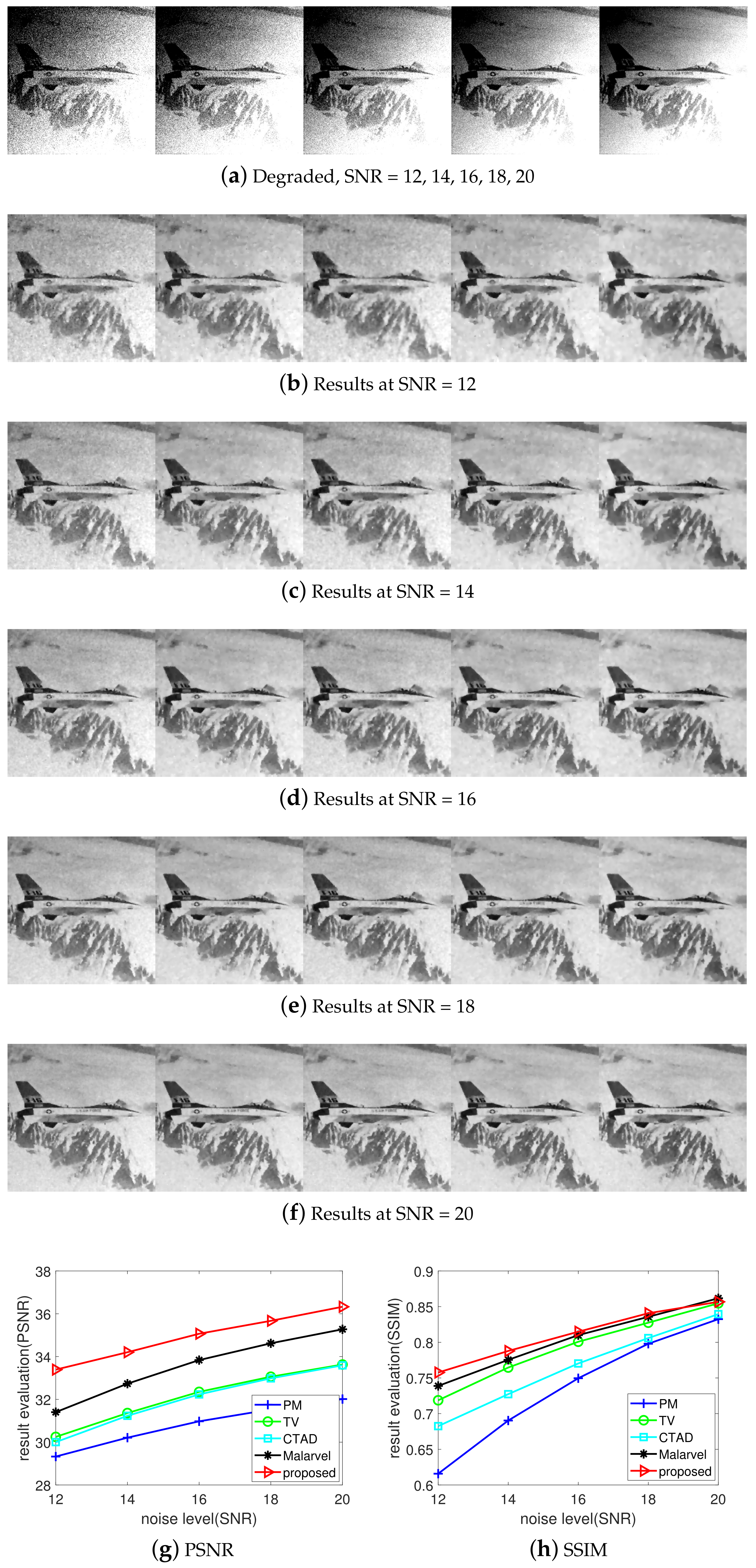
Figure 1d, the clear image is polluted by Gaussian noise (Signal to Noise Ratio, SNR = 20) and an inconsistent background. The top-left seems underexposed, and the bottom-right looks overexposed. With PM model performance, the noise removal and edge preservation can be well balanced under the influence of an inconsistent background (as shown in
Figure 1e). Applying our model on the degraded image, noise and inconsistent background are both reduced while the edge is preserved (as shown in
Figure 1f). The PSNR curve and SSIM curve are shown in
Figure 1g,h.
3.2. Numerical Scheme
In this paper, the spatial domain is discretized by a grid domain and the time interval is discretized as . Then the numerical solution of at can be denoted as .
Apply the minmod scheme [
1]
to approximate the TV diffusion terms, and apply central difference to approximate all other differential term, then an efficient numerical scheme for the proposed model (
14) can be denoted as
Here,
is denoted as
and the Lagrange multipliers can be determined by
or
After discretization of the boundary condition and initial condition by the central difference scheme, the numerical algorithm can be implemented efficiently.


