Abstract
The performance of a typical solar energy-based system can be improved by accurately modeling the current versus voltage characteristics of the involved solar cells. However, estimating the exact value of parameters related to solar cells is quite challenging. The optimization function, considering the current–voltage characteristics of solar cells, requires the solution of sophisticated non-linear and multi-modal optimization methods. So far, various optimization approaches have been reported. This paper proposes the application of a new hybrid algorithm, i.e., Particle Swarm Optimization and Gravitational Search Algorithm (PSOGSA), which is a combination of two algorithms, i.e., Gravitational Search Algorithm (GSA) and Particle Swarm Optimization (PSO) method. The hybrid PSOGSA algorithm is superior to other algorithms in terms of higher accuracy in searching for optimal solutions and better explorative capability. Moreover, the developed hybrid algorithm is benchmarked using ten standard test functions to verify its efficiency. In this manuscript, monocrystalline and polycrystalline solar cells are considered. The parameter optimization results are obtained using PSOGSA and further compared with those obtained using other algorithms presented in the literature, such as PSO, GSA, MVO, HBO, PO and SCA. The complete error analysis is carried out for the modified single-diode model (MSDM), the modified double-diode model (MDDM), and the modified three-diode model (MTDM) of photovoltaic (PV) cells to prove the superiority of the PSOGSA. Moreover, statistical results are carried out based on Friedman’s ranking and Wilcoxon’s rank sum test. The comparison results show that the proposed PSOGSA is better than other algorithms in estimating the unknown PV model parameters.
Keywords:
PV modeling; single-diode; double-diode; three-diode; PSOGSA; error analysis; non-parametric tests 1. Introduction
1.1. Literature Review
Solar photovoltaic (PV) systems are eco-friendly and help to minimize the greenhouse gas (GHG) emission gases that would otherwise have emerged from the use of fossil fuels for generating electricity. Since solar energy is available in abundance, feeding electricity into the grid through solar PV plants can help in transmitting the much larger amounts of power that might be made from the GHG-intensive network. The increased cost of the PV modules restricts the optimum and maximum utilization of the available renewable energy. Thus, the system’s reliability and accuracy in simulated environments must be predicted before the system is actually installed.
Modeling solar cells is essential to predict the behavior of the actual solar cell under different environmental conditions and further acquire its characteristic curves; the current–voltage and power–voltage curves. The viable method is to use the analogous electrical circuit, which is based entirely on a source of light-generated current connected to a p–n junction diode. Many frameworks have been developed at different solar intensities and temperature conditions for the simulation of a single solar cell or a complete PV system [1,2,3,4]. Thus, effective and precise solar cell modeling is very crucial to predict its behavior under different atmospheric conditions. Effective modeling of the non-linear characteristics of the PV systems is very beneficial from the point of accurate simulation [5]. In literature, there are various types of stochastic approaches described in the past few decades, such as single-diode, two-diode, and three-diode models, designs with partial shading issues, and many more.
The mathematical model of I-V characteristics of PV cells contains a large number of unknown factors. The single and double-diode models are the leading theoretical frameworks for the precise modeling of the system [6]. The single-diode structure is represented by its simplicity and highly acceptable accuracy [7,8]. The I-V performance feature of the single-diode model has five unknown parameters, i.e., PV current, diode saturation current, ideality factor, parallel and series resistances [9]. This model, however, lacks precision at low irradiance open-circuit voltage as the carrier recombination losses in the depletion region seem to be ignored [10,11]. To overcome this problem, the double-diode model was introduced. In this model, to represent the recombination losses, an extra diode is used. This model shows better accuracy than the single-diode model. However, it is more complicated than a single-diode model because seven parameters need to be evaluated in the two-diode model in contrast to five parameters in a single-diode model [11,12,13]. The three-diode model exhibits better accuracy than the two-diode model, which affects the leakage current and grain boundaries [14]. The three-diode model involves the estimation of nine parameters which is somewhat more complicated than the two-diode model [15].
Hybridizing stochastic optimization algorithms is one of the best ways to develop superior algorithms and exploit numerous algorithm advantages for solving optimization problems [16,17,18,19,20]. In 2010, the PSOGSA algorithm was proposed, which is a novel hybrid of the PSO technique and GSA algorithm [21]. This algorithm shows a better outcome in solving optimization problems. In this algorithm, agents perform the search process, mimicking GSA behavior in the phase of exploration, and PSO in the exploitation phase. This algorithm was initially introduced to mitigate the GSA’s slow exploitation and also mitigate the PSO algorithm’s nature to get struck in local minima, which are their key drawbacks. Many studies have been undertaken to improve the performance of the GSA algorithm as well as the PSO algorithm. For solving the clustering problem, the hybrid PSOGSA proved to be the better method for solving the heuristic problems [22].
Many researchers are experimenting with different applications by developing new algorithms such as the Skill optimization algorithm [23], Equilibrium optimization [24] and so on. In this manuscript, an engineering application is presented using a hybrid algorithm, that is, the Particle Swarm Optimization and Gravity Search Algorithm (PSOGSA), to estimate the parameters of monocrystalline solar cells and polycrystalline cells. The results obtained using PSOGSA are compared with those obtained using Particle Swarm Optimization (PSO) [25], Gravitational Search Algorithm (GSA) [26], Multi-Verse Optimizer (MVO) [27], Sine Cosine Algorithm (SCA) [28], Heap Based Optimizer (HBO) [29], and Political Optimizer (PO) [30]-based techniques to check the effectiveness of the PSOGSA.
1.2. Paper Contribution
The main contributions of this work are summarized as follows:
- A new hybrid (PSOGSA) algorithm is proposed to estimate the unknown parameters of a single, double and triple-diode model for two different solar PV cells.
- Ten benchmark test functions are selected to justify the performance of the proposed hybrid algorithm.
- Different objective functions are implemented for extracting the solar PV cell parameters such as SSE, AE, MAE, MSE and RMSE functions.
- Comprehensive statistical analysis and comparisons of the hybrid algorithm with other metaheuristic optimization algorithms.
- Focusing on solution consistency results, I-V and P-V characteristic curves, non-parametric tests are also implemented.
1.3. Paper Organization
This work is arranged as follows: Section 2 presents the mathematical modeling of different PV cells. In Section 3, the problem formulation is proposed. Section 4 introduces the suggested hybrid PSOGSA algorithm and its steps. Section 5 depicts the simulation results, comparisons and statistical metrics. Finally, Section 6 draws conclusions and recommendations for further work.
2. Mathematical Modeling of PV Cell
The modeling of solar PV cells can be accomplished by a comprehensive study of mathematical equations based on the respective analogous circuits of solar PV models described in the following subsections [31,32,33,34].
2.1. Ideal Solar PV Cell Modeling
The ideal solar PV cells with photocurrent (Iph) vary from the optimal outcome because of optical and electrical losses. Figure 1 represents a typical solar PV cell, which is the simplest PV model as the effect of parallel and series resistances is not reckoned.
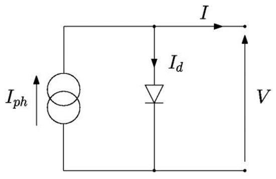
Figure 1.
Equivalent circuit of an ideal solar PV cell.
The cell output is expressed by I-V characteristics and expressed in mathematical terms as follows:
where Id signifies the diode current, which represents the recombination and diffusion current in the quasi steady-state emitter region and PN junction region with excess concentration. This current in the diode is represented by the Shockley Equation as follows:
where Io represents the saturation diode current, Vd is known as the diode voltage, Vt is the equivalent thermal voltage and N is the number of cells in series [35]. An ideal solar photovoltaic cell does not take into account the effects of internal resistance, and thus does not establish a stable relationship between the cell current and voltage.
2.2. Modified Equivalent Circuit of the Single-Diode PV Model
The ideal PV cell model can also be introduced by a series resistance to get accurate results. This model is simple because it reveals deficiencies when subjected to variations in temperature [36]. The refined version of the single-diode model (SDM) is the modified single-diode model (MSDM). In the MSDM, additional resistance is incorporated in series with the basic SDM which expresses the losses in the quasi-neutral region as shown in Figure 2. Equation (3) represents the modeling of a modified single-diode cell as follows:
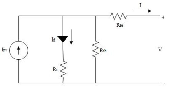
Figure 2.
Schematic diagram of the modified single-diode PV model.
2.3. Modified Equivalent Circuit of the Double-Diode PV Model
The refined version of the double-diode model (DDM) is the modified double-diode model (MDDM). In the MDDM, additional resistance is incorporated in series with the basic DDM which represents that the resistance at grain boundaries is greater than resistance within crystallites. The accuracy of the modified single-diode model is uncertain; therefore, further investigation was carried out to search for more sophisticated models. A modified two-diode model is adopted to solve this problem, using two diodes attached parallel to the current source, as shown in Figure 3. The modified double-diode model is the modified version of the modified single-diode model, which takes the effect of recombination into account by introducing another diode in parallel.
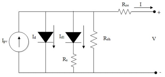
Figure 3.
Schematic diagram of the modified double-diode PV model.
In this model, two unknown diode-quality factors are introduced. As a result, there is an increase in the number of equations which makes calculations more complicated [37]. Hence, at a low insolation level, this model exhibits better accuracy. Equation (4) represents the performance equation of the modified double-diode cell model.
Therefore, considering all aspects of mathematical calculation, and the number of iterations, the modified single-diode model tends to have quick results due to fewer complex calculations.
2.4. Modified Equivalent Circuit of the Triple-Diode PV Model
The refined version of the triple-diode model (TDM) is the modified triple-diode model (MTDM). In the MTDM, additional resistance is incorporated in series with the basic TDM. Moreover, the losses in the defect area are represented by adding a modified series resistance i.e., Rs. Figure 4 represents the modified three-diode equivalent circuit model for a PV cell in which there are three diodes. The effect of the leakage current and grain boundaries represented by Id3 has been taken into account in this model. In this model, the current through the shunt resistance branch is the leakage current. The semiconductor material resistance signifies a series resistance in the natural region of the solar cell [15]. Equation (5) represents the performance equation of the modified three-diode equivalent model of the solar PV cell.
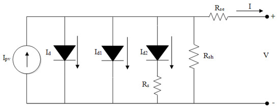
Figure 4.
Schematic diagram of the modified triple-diode PV model.
3. Problem Formulation
This section presents the problem formulation that has been implemented to extract the parameters of different PV solar cells. To evaluate the characteristics of the solar cells, different objective functions have been carried out in this paper such as: the sum of square error (SSE), absolute error (AE), mean absolute error (MAE), mean square error (MSE) and the root mean square error (RMSE). However, RMSE is the most common formula used to estimate the unknown parameters of the PV cells [9,15]. The RMSE between the measured and calculated output current of the solar cell can be calculated as follows:
where represents the number of measured points, and represent the measured and calculated solar cell current at point , respectively. Moreover, the other error functions can be calculated using the following equations:
where is the mean value of all the measured cell currents. The prime objective of the presented technique is to extract the parameters of the modified-diode model by minimizing the root mean square error. Hence, the proposed approach will be used on the basis of minimizing this objective function with respect to the parameter limits.
4. The Proposed Hybrid PSOGSA Algorithm
This manuscript has identified the supremacy of the hybrid PSOGSA algorithm compared to other algorithms such as PSO [30], GSA [31], MVO [32], SCA [33], HBO [34], and PO [35] techniques. Using the modified single-diode, the modified double-diode, and the modified three-diode identical models, these algorithms have been used to optimize the parameters of monocrystalline and polycrystalline PV cells.
In general, the hybrid PSOGSA combines the exploitation ability of the PSO algorithm and the exploration ability of the GSA algorithm to obtain optimal results more effectively. This provides a better balance between the two algorithms for an optimal solution. Mirjalili and Mohd Hashim first introduced the hybrid PSOGSA algorithm [21]. The best solution achieved using the PSO algorithm is saved for further exploration in the GSA algorithm. The purpose of using the best solution is that GSA suffers from regression and exploitation delays in the initial iterations [38]. The PSOGSA has been shown to be effective enough to find the optimal solution compared to the PSO and GSA techniques. However, the primitive hybrid algorithm PSOGSA is a continuous algorithm that is not explicitly capable of solving binary problems. The flowchart of the hybrid PSOGSA algorithm is represented in Figure 5 and the steps are described below.
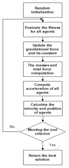
Figure 5.
The hybrid PSOGSA algorithm flowchart.
Step 1: In this step, the acceleration and position of all the particles are first initialized.
Step 2: According to Equation (11), the fitness values of all particles are found and updated for their constant gravity. In Equation (11), Gt and Go stand for the gravitational constant of the universe at the moment t and to, respectively. T stands for the maximum number of iterations.
Step 3: In this step, the quality of the particle is obtained according to Equations (12)–(14). Using Equations (15)–(17), the acceleration of the particle is found. Lit stands for the fitness value in Equations (14) and (15).
F = G (M1M2/R)
a = F/M
Equation (16) obeys the law of gravity, and Equation (17) follows the law of motion. The maximum number of iterations is set to 1000 whereas the search agents are kept at 30 for all the algorithms.
Step 4: In this step, the position and velocity of the particle are calculated, and updated according to the position and velocity in Equation (19).
where M1 and M2 are two positive constants of acceleration; rand () is a uniform random number (0, 1); Pdi and Pdg are the best positions so far found by the ith particle and all the particles, respectively; t is the iteration count; and is an inertial weight that usually decreases linearly during the iterations. The weight of inertia is used to balance local and global searches [39].
Xdi (t + 1) = Vdi (t + 1) + Xdi (t)
Step 5: This is the last step of the algorithm. If the system has met the criteria, then the output is optimum; otherwise go back to step 2.
5. Results and Discussion
5.1. Benchmark Test Functions
In this section, the developed hybrid algorithm (PSOGSA) is benchmarked using ten standard test functions to verify its efficiency. The characteristics of these benchmark test functions are summarized in Table 1 [40,41]. The functions to are unimodal functions that are mainly used to investigate the convergence characteristics and optimization accuracy of a given algorithm. Moreover, the functions to are multimodal functions that are mainly used to check whether an algorithm can avoid precocity and find global optimal solutions [40,41]. Each function dimension (n) is set to 30 to avoid random interference.

Table 1.
Definitions of benchmark functions.
For performance verification, the hybrid PSOGSA algorithm is compared with other optimization algorithms such as MVO, PSO, SCA, HBO, PO and GSA. The results of the benchmark functions are summarized in Table 2 based on the mean value and standard deviation (std) values for each function. It can be observed from Table 2 that the hybrid PSOGSA algorithm is superior to other algorithms in terms of higher accuracy in searching for optimal solutions and better explorative capability.
Table 2.
Results of benchmark test functions for different optimization algorithms.
5.2. Parameter Estimation Results
Two solar cells are used to estimate the parameters i.e., Monocrystalline and Polycrystalline, as shown in Table 3. In this section, the two cases are discussed in which the modified single-diode, the modified double-diode and the modified three-diode model parameter estimations have been carried out.
Table 3.
Datasheet for two different types of PV cells.
Each algorithm is set to a maximum number of 1000 iterations and with 40 search agents using MATLAB version 19b. All algorithms are repeated 30 times and the result of each is recorded. After estimating the parameters based on different errors, the statistical results such as the mean and standard deviation are calculated and compared with those obtained using different algorithms for 30 error values. The standard deviation can be calculated using Equation (20) as follows:
where is the number of error values (), and and represent the error calculated using each algorithm and the mean error value, respectively.
It has been observed that the developed hybrid PSOGSA algorithm gives better results compared to those obtained with the other algorithms considered in this work. Figure 6 and Figure 7 show the I-V and P-V curves at standard temperature conditions. After calculating the error, the non-parametric test is also conducted. The first non-parametric test performed is the Wilcoxon rank sum test which is explained in detail in [42,43,44]. After this test, the Friedman rank test is performed to see how accurate the newly developed hybrid algorithm is better than the other comparative algorithms. For parameter estimation of different types of the PV diode modeling, two cases are considered below:
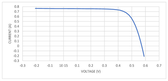
Figure 6.
The I-V curve at standard temperature conditions.
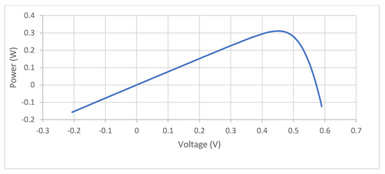
Figure 7.
The P-V curve at standard temperature conditions.
Case 1: The solar cell is considered monocrystalline in this case. This case is further divided into three parts as follows:
- Modified Single-Diode Model (MSDM):Table 4 shows the results of parameter estimation using different optimization algorithms. Figure 8 represents the MSDM convergence curve. From this curve, we conclude that the efficiency of the proposed algorithm is better than the rest of the comparative algorithms. The errors, mean, and standard deviation of the MSDM circuit equivalent of a PV cell are shown in Table 5. Based on the results, it can be inferred that parameter estimation using the developed hybrid PSOGSA is superior to other comparative algorithms.
Table 4. The monocrystalline MSDM parameter estimation results.
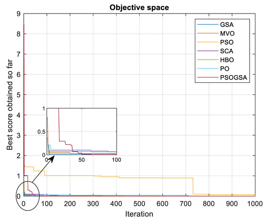 Figure 8. The convergence curve of the monocrystalline MSDM.
Table 5. The MSDM calculation error, mean and standard deviation for the monocrystalline PV cell.
Figure 8. The convergence curve of the monocrystalline MSDM.
Table 5. The MSDM calculation error, mean and standard deviation for the monocrystalline PV cell. - Modified Double-Diode Model (MDDM): Table 6 shows the results of parameter estimation using different optimization algorithms. Figure 9 represents the convergence curve for MDDM. It was concluded that the efficiency of the proposed algorithm is better than the rest of the comparative algorithms. The errors, mean, and standard deviation of the MDDM circuit equivalent to a PV cell are shown in Table 7. Based on the results, it can be concluded that parameter estimation using the developed hybrid PSOGSA is superior to other algorithms.
Table 6. The monocrystalline MDDM parameter estimation results.
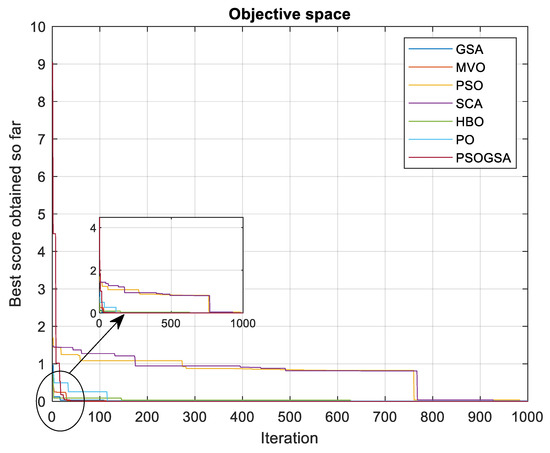 Figure 9. The convergence curve of the monocrystalline MDDM.
Table 7. The MDDM calculation error, mean and standard deviation for the monocrystalline PV cell.
Figure 9. The convergence curve of the monocrystalline MDDM.
Table 7. The MDDM calculation error, mean and standard deviation for the monocrystalline PV cell. - The Modified Triple-Diode Model (MTDM): Table 8 shows the results of parameter estimation using different optimization algorithms. Figure 10 represents the convergence curve of the MTDM that proves the efficiency of the proposed algorithm over other algorithms. The errors, mean, and standard deviation of the MTDM circuit equivalent to a PV cell are shown in Table 9. Based on the results, it can be inferred that parameter estimation using the developed hybrid PSOGSA is superior to other algorithms.
Table 8. The monocrystalline MTDM parameter estimation results.
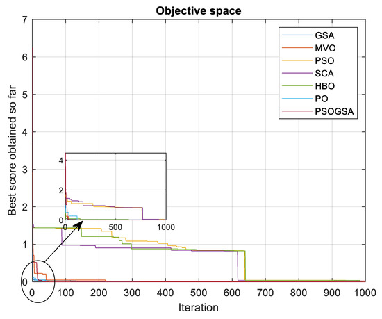 Figure 10. The convergence curve of the monocrystalline MTDM.
Table 9. The MTDM calculation error, mean and standard deviation for the monocrystalline PV Cell.
Figure 10. The convergence curve of the monocrystalline MTDM.
Table 9. The MTDM calculation error, mean and standard deviation for the monocrystalline PV Cell. - Non-Parametric Test: Non-parametric tests are performed to justify the results obtained by all algorithms. Table 10 represents the statistical result based on the Wilcoxon rank sum test. Friedman’s rank test is represented in Table 11. Based on the results of this test, it is clear that the newly generated hybrid algorithm is more reliable and superior to other similar algorithms. Based on the results of both tests, it is clear that PSOGSA is superior to other compared algorithms.
Table 10. Statistical results based on Wilcoxon’s rank sum test for the monocrystalline PV Cell.
Table 11. Friedman ranking test’s statistical result for the monocrystalline PV Cell.
Case 2: This case is also divided into three parts as follows for the polycrystalline PV solar cell:
- Modified Single-diode Model (MSDM):Table 12 shows the results of parameter estimation using different optimization algorithms. Figure 11 represents the convergence curve of the MSDM. From this convergence curve, it is concluded that the efficiency of the proposed algorithm is better than the rest of the compared algorithms. The errors, mean, and standard deviation of the MSDM circuit equivalent to a PV cell are shown in Table 13. Based on the results, it can be inferred that parameter estimation using the developed hybrid PSOGSA is superior to other algorithms.
Table 12. Parameter Estimation of the MSDM for the polycrystalline PV Cell.
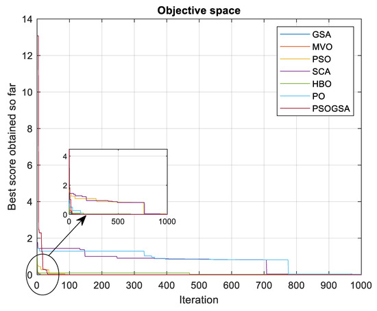 Figure 11. The convergence curve of the polycrystalline MSDM.
Table 13. The MSDM calculation error, mean, standard deviation for the polycrystalline PV Cell.
Figure 11. The convergence curve of the polycrystalline MSDM.
Table 13. The MSDM calculation error, mean, standard deviation for the polycrystalline PV Cell. - Modified Double-Diode Model (MDDM):Table 14 shows the results of parameter estimation using different optimization algorithms. Figure 12 represents the convergence curve of the MDDM for this case. The errors, mean, and standard deviation of the MDDM circuit equivalent to a PV cell are shown in Table 15. Based on the results, it can be concluded that parameter estimation using the developed hybrid PSOGSA is superior to other algorithms.
Table 14. Results of parameter estimation of the MDDM for the polycrystalline PV Cell.
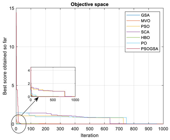 Figure 12. The convergence curve of the polycrystalline MDDM.
Table 15. The MDDM calculation error, mean and standard deviation for Case 2.
Figure 12. The convergence curve of the polycrystalline MDDM.
Table 15. The MDDM calculation error, mean and standard deviation for Case 2. - The Modified Three-Diode Model (MTDM): Table 16 shows the results of parameter estimation using different optimization algorithms. Figure 13 represents the convergence curve for Case 2 that proves the efficiency of the proposed algorithm. The errors, mean, and standard deviation of the MTDM circuit equivalent to a PV cell are shown in Table 17. Based on the results, it can be inferred that parameter estimation using the developed hybrid PSOGSA is superior to other algorithms.
Table 16. Results of parameter estimation of the MTDM for Case 2.
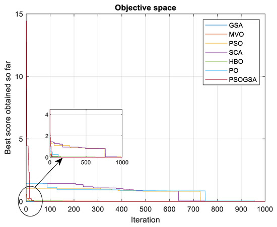 Figure 13. The convergence curve of the polycrystalline MTDM.
Table 17. The MTDM calculation error, mean and standard deviation for Case 2.
Figure 13. The convergence curve of the polycrystalline MTDM.
Table 17. The MTDM calculation error, mean and standard deviation for Case 2. - Non-Parametric Test: Non-parametric tests are performed to justify the results obtained by all algorithms. Table 18 represents the statistical result based on the Wilcoxon rank sum test. The Friedman rank test is represented in Table 19. Based on the results of this test, it is clear that the newly generated hybrid algorithm is more reliable and superior to other similar algorithms. Based on the results of both tests, PSOGSA clearly outperforms the other algorithms.
Table 18. Wilcoxon’s rank sum test for Case 2.
Table 19. Friedman’s ranking test for Case 2.
6. Conclusions
The abundant availability of solar energy has attracted many efforts to exploit it as much as possible to meet the energy needs of humans. In this work, two types of solar photovoltaic cells were considered: the monocrystalline cell and the polycrystalline cell. Various mathematical equivalent models of the photovoltaic cell such as MSDM, MDDM and MTDM were explored in this work. For efficient parameter estimation in the considered models for both types of photovoltaics, a hybrid algorithm such as (PSOGSA) was tested, which is a combination of two algorithms, the particle swarm optimization and gravity search algorithm. In terms of exploration and exploitation, the hybrid algorithm is superior to both algorithms. Results obtained using PSOGSA were compared with those obtained using PSO, GSA, MVO HBO, PO and SCA techniques. The PSOGSA method clearly showed more promising results compared to any of the other algorithms considered in this work. Various errors such as SSE, AE, MAE, MSE, RMSE, were also calculated and the average, standard deviation is calculated after estimating the MSDM, MDDM and MTDM parameters of monocrystalline and polycrystalline solar PV cells. Full error analysis justified the superiority of PSOGSA in parameter estimation of solar PV cells over other algorithms considered in this work. To get a better accuracy of the hybrid algorithm, statistical results were also carried out, and through testing theses, it is clear that the proposed hybrid algorithm is better than the rest of the comparative algorithms. These studies have demonstrated that the hybrid algorithm (PSOGSA) is a promising and efficient method for modified solar PV parameter extraction as it increases the efficiency of the solar panel, proving that the same amount of power can be generated from the same solar panel by reducing the internal loses. For future studies, the hybrid algorithm can be used for establishing a dynamic model of the PV panel.
Author Contributions
Methodology, J.G., W.H. and K.M.A.; Software, M.K.S. and W.H.; Validation, J.G. and A.H.; Formal analysis, A.H., P.N. and H.K.; Investigation, J.G., A.H., M.K.S., W.H. and K.M.A.; Resources, H.K.; Writing—review & editing, M.K.S., P.N. and K.M.A.; Visualization, P.N. and K.M.A.; Supervision, K.M.A.; Funding acquisition, H.K. All authors have read and agreed to the published version of the manuscript.
Funding
This research received no external funding.
Institutional Review Board Statement
Not applicable.
Informed Consent Statement
Not applicable.
Data Availability Statement
The data sources employed for analysis are presented in the text.
Conflicts of Interest
The authors declare no conflict of interest.
References
- Saloux, E.; Teyssedou, A.; Sorin, M. Explicit model of photovoltaic panels to determine voltages and currents at the maximum power point. Sol. Energy 2011, 85, 713–722. [Google Scholar] [CrossRef]
- Ishaque, K.; Salam, Z.; Taheri, H. Simple, fast and accurate two-diodemodel for photovoltaic modules. Sol. Energy Mater. Sol. Cells 2011, 95, 586–594. [Google Scholar] [CrossRef]
- Tsai, H.L. Insolation-oriented model of photovoltaic module using Matlab/Simulink. Sol. Energy 2010, 84, 1318–1326. [Google Scholar] [CrossRef]
- Gow, J.A.; Manning, C.D. Development of a photovoltaic array model for use in power-electronics simulation studies. IEEE Proc.-Electr. Power Appl. 1999, 146, 193–200. [Google Scholar] [CrossRef]
- Yetayew, T.T.; Jyothsna, T.R. Improved single-diode modeling approach for photovoltaic modules using data sheet. In Proceedings of the 2013 Annual IEEE India Conference (INDICON), Mumbai, India, 13–15 December 2013; pp. 1–6. [Google Scholar]
- Chin, V.J.; Salam, Z.; Ishaque, K. Cell modelling and model parameters estimation techniques for photovoltaic simulator application: A review. Appl. Energy 2015, 154, 500–519. [Google Scholar] [CrossRef]
- Mahmoud, Y.; El-Saadany, E.F. A photovoltaic model with reduced computational time. IEEE Trans. Ind. Electron. 2014, 62, 3534–3544. [Google Scholar] [CrossRef]
- Hasanien, H.M. Shuffled frog leaping algorithm for photovoltaic model identification. IEEE Trans. Sustain. Energy 2015, 6, 509–515. [Google Scholar] [CrossRef]
- AlHajri, M.F.; El-Naggar, K.M.; AlRashidi, M.R.; Al-Othman, A.K. Optimal extraction of solar cell parameters using pattern search. Renew. Energy 2012, 44, 238–245. [Google Scholar] [CrossRef]
- Lim, L.H.I.; Ye, Z.; Ye, J.; Yang, D.; Du, H. A linear identification of diode models from single I–V characteristics of PV panels. IEEE Trans. Ind. Electron. 2015, 62, 4181–4193. [Google Scholar] [CrossRef]
- Shannan, N.M.A.A.; Yahaya, N.Z.; Singh, B. Single-diode model and two-diode model of PV modules: A comparison. In Proceedings of the 2013 IEEE International Conference on Control System, Computing and Engineering, Penang, Malaysia, 29 November–1 December 2013; pp. 210–214. [Google Scholar]
- Gupta, S.; Tiwari, H.; Fozdar, M.; Chandna, V. Development of a two diode model for photovoltaic modules suitable for use in simulation studies. In Proceedings of the 2012 Asia-Pacific Power and Energy Engineering Conference, Shanghai, China, 26–28 March 2012; pp. 1–4. [Google Scholar]
- Kassis, A.; Saad, M. Analysis of multi-crystalline silicon solar cells at low illumination levels using a modified two-diode model. Sol. Energy Mater. Sol. Cells 2010, 94, 2108–2112. [Google Scholar] [CrossRef]
- Nishioka, K.; Sakitani, N.; Uraoka, Y.; Fuyuki, T. Analysis of multicrystalline silicon solar cells by modified 3-diode equivalent circuit model taking leakage current through periphery into consideration. Sol. Energy Mater. Sol. Cells 2007, 91, 1222–1227. [Google Scholar] [CrossRef]
- Elazab, O.S.; Hasanien, H.M.; Elgendy, M.A.; Abdeen, A.M. Parameters estimation of single-and multiple-diode photovoltaic model using whale optimisation algorithm. IET Renew. Power Gener. 2018, 12, 1755–1761. [Google Scholar] [CrossRef]
- Esmin, A.A.A.; Lambert-Torres, G.; Alvarenga, G.B. Hybrid evolutionary algorithm based on PSO and GA mutation. In Proceedings of the 2006 Sixth International Conference on Hybrid Intelligent Systems (HIS’06), Auckland, New Zealand, 14–16 December 2006; p. 57. [Google Scholar]
- Holden, N.; Freitas, A.A. A hybrid PSO/ACO algorithm for discovering classification rules in data mining. J. Artif. Evol. Appl. 2008, 2008, 1–11. [Google Scholar] [CrossRef]
- Holden, N.P.; Freitas, A.A. A hybrid PSO/ACO algorithm for classification. In Proceedings of the 9th Annual Conference Companion on Genetic and Evolutionary Computation, London, UK, 7–11 July 2007; pp. 2745–2750. [Google Scholar]
- Lai, X.; Zhang, M. An efficient ensemble of GA and PSO for real function optimization. In Proceedings of the 2009 2nd IEEE International Conference on Computer Science and Information Technology, Beijing, China, 8–11 August 2009; pp. 651–655. [Google Scholar]
- Niu, B.; Li, L. A novel PSO-DE-based hybrid algorithm for global optimization. In Proceedings of the International Conference on Intelligent Computing, Shanghai, China, 15–18 September 2008; pp. 156–163. [Google Scholar]
- Mirjalili, S.; Hashim, S.Z.M. A new hybrid PSOGSA algorithm for function optimization. In Proceedings of the 2010 International Conference on Computer and Information Application, Austin, TX, USA, 6–10 December 2010; pp. 374–377. [Google Scholar]
- Hatamlou, A.; Abdullah, S.; Othman, Z. Gravitational search algorithm with heuristic search for clustering problems. In Proceedings of the 2011 3rd Conference on Data Mining and Optimization (DMO), Putrajaya, Malaysia, 28–29 June 2011; pp. 190–193. [Google Scholar]
- Fathy, A.; Rezk, H.; Ferahtia, S.; Ghoniem, R.M.; Alkanhel, R.; Ghoniem, M.M. A New Fractional-Order Load Frequency Control for Multi-Renewable Energy Interconnected Plants Using Skill Optimization Algorithm. Sustainability 2022, 14, 14999. [Google Scholar] [CrossRef]
- Abdelrazek, A.S.; El-Sehiemy, R.A.; Rezk, H.; Ghoniem, R.M.; Falaras, P.; Zaky, A.A. Dynamic Electrical Models of Perovskite Solar Cells Considering Hysteresis and Charge Accumulations Effects by Using Equilibrium Optimizer. IEEE Access 2022, 10, 104111–104122. [Google Scholar] [CrossRef]
- Wang, Y.; Li, B.; Weise, T.; Wang, J.; Yuan, B.; Tian, Q. Self-adaptive learning based particle swarm optimization. Inf. Sci. 2011, 181, 4515–4538. [Google Scholar] [CrossRef]
- Rashedi, E.; Nezamabadi-Pour, H.; Saryazdi, S. GSA: A gravitational search algorithm. Inf. Sci. 2009, 179, 2232–2248. [Google Scholar] [CrossRef]
- Mirjalili, S.; Mirjalili, S.M.; Hatamlou, A. Multi-verse optimizer: A nature-inspired algorithm for global optimization. Neural Comput. Appl. 2016, 27, 495–513. [Google Scholar] [CrossRef]
- Bellia, H.; Youcef, R.; Fatima, M. A detailed modeling of photovoltaic module using MATLAB. NRIAG J. Astron. Geophys. 2014, 3, 53–61. [Google Scholar] [CrossRef]
- Benlarbi, K.; Mokrani, L.; Nait-Said, M.S. A fuzzy global efficiency optimization of a photovoltaic water pumping system. Sol. Energy 2004, 77, 203–216. [Google Scholar] [CrossRef]
- Arab, A.H.; Chenlo, F.; Benghanem, M. Loss-of-load probability of photovoltaic water pumping systems. Sol. Energy 2004, 76, 713–723. [Google Scholar] [CrossRef]
- Sera, D.; Teodorescu, R.; Rodriguez, P. PV panel model based on datasheet values. In Proceedings of the 2007 IEEE International Symposium on Industrial Electronics, Edinburgh, UK, 19–21 June 2007; pp. 2392–2396. [Google Scholar]
- Mirjalili, S. SCA: A sine cosine algorithm for solving optimization problems. Knowl.-Based Syst. 2016, 96, 120–133. [Google Scholar] [CrossRef]
- Askari, Q.; Saeed, M.; Younas, I. Heap-based optimizer inspired by corporate rank hierarchy for global optimization. Expert Syst. Appl. 2020, 161, 113702. [Google Scholar] [CrossRef]
- Askari, Q.; Younas, I.; Saeed, M. Political optimizer: A novel socio-inspired meta-heuristic for global optimization. Knowl.-Based Syst. 2020, 195, 105709. [Google Scholar] [CrossRef]
- Sheik Mohammed, S.; Devaraj, D. Interleaved boost converter with perturb and observe maximum power point tracking algorithm for photovoltaic system. In Proceedings of the International Conference on Substantial Environmental Engineering and Renewable Energy, Abu Dhabi, United Arab Emirates, 13–14 January 2015. [Google Scholar]
- Jain, A.; Kapoor, A. Exact analytical solutions of the parameters of real solar cells using Lambert W-function. Sol. Energy Mater. Sol. Cells 2004, 81, 269–277. [Google Scholar] [CrossRef]
- Ma, T.; Yang, H.; Lu, L. Development of a model to simulate the performance characteristics of crystalline silicon photovoltaic modules/strings/arrays. Sol. Energy 2014, 100, 31–41. [Google Scholar] [CrossRef]
- Mirjalili, S.; Hashim, S.Z.M.; Sardroudi, H.M. Training feedforward neural networks using hybrid particle swarm optimization and gravitational search algorithm. Appl. Math. Comput. 2012, 218, 11125–11137. [Google Scholar] [CrossRef]
- Tsai, C.Y.; Chiu, C.C. Developing a feature weight self-adjustment mechanism for a K-means clustering algorithm. Comput. Stat. Data Anal. 2008, 52, 4658–4672. [Google Scholar] [CrossRef]
- Xue, H.; Bai, Y.; Hu, H.; Xu, T.; Liang, H. A Novel Hybrid Model Based on TVIW-PSO-GSA Algorithm and Support Vector Machine for Classification Problems. IEEE Access 2019, 7, 27789–27801. [Google Scholar] [CrossRef]
- Singh, B.; Singla, M.K.; Nijhawan, P. Parameter Estimation of Four Diode Solar Photovoltaic Cell Using Hybrid Algorithm. Energy Sources Recovery Util. Environ. Eff. 2022, 44, 4597–4613. [Google Scholar] [CrossRef]
- Singla, M.K.; Nijhawan, P. Triple diode parameter estimation of solar PV cell using hybrid algorithm. Int. J. Environ. Sci. Technol. 2021, 19, 4265–4288. [Google Scholar] [CrossRef]
- Singla, M.K.; Nijhawan, P.; Oberoi, A.S. Parameter estimation of proton exchange membrane fuel cell using a novel meta-heuristic algorithm. Environ. Sci. Pollut. Res. 2021, 28, 34511–34526. [Google Scholar] [CrossRef] [PubMed]
- Gupta, J.; Nijhawan, P.; Ganguli, S. Parameter estimation of different solar cells using a novel swarm intelligence technique. Soft Comput. 2022, 26, 5833–5863. [Google Scholar] [CrossRef]


Disclaimer/Publisher’s Note: The statements, opinions and data contained in all publications are solely those of the individual author(s) and contributor(s) and not of MDPI and/or the editor(s). MDPI and/or the editor(s) disclaim responsibility for any injury to people or property resulting from any ideas, methods, instructions or products referred to in the content. |
© 2022 by the authors. Licensee MDPI, Basel, Switzerland. This article is an open access article distributed under the terms and conditions of the Creative Commons Attribution (CC BY) license (https://creativecommons.org/licenses/by/4.0/).