The Impact of the Temperature Control Strategy in Steady-State Virtual Vacuum Simulation on the Spontaneous Evaporation Rate and Corresponding Evaporation Coefficient

Abstract

In the present paper, we propose a novel simulation approach that allows one to capture the steady-state evaporation into virtual vacuum state by maintaining a constant number of atoms within the liquid phase during the simulations. The proposed method was used to perform virtual vacuum simulations of argon at a temperature of 90 K in order to study the effects of the chosen simulation temperature control approach on the system’s temperature profiles, spontaneous evaporation rates, and the energetic characteristics of the evaporating atoms. The results show that the expected non-uniform temperature profile across the liquid phase can be flattened out by dividing the liquid phase into separately thermostated bins. However, the desired liquid surface temperature can be achieved only when the thermostat region boundary is placed outside the liquid phase. The obtained relationship between the surface temperature and the spontaneous evaporation rate show that the spontaneous evaporation rate and corresponding evaporation coefficient evaluation may change up to 21% when the surface temperature changes in a narrow temperature interval of 2.45 K. Furthermore, the results demonstrate that the thermostat region boundary position has no impact on the energetic characteristics of the evaporating argon atoms, even when the boundary is placed outside the liquid phase.

1. Introduction

With advancements in the field of nanotechnology, two-phase liquid-vapor problems are increasingly more present in a wide range of nanofluidic processes, such as capillary evaporation, condensation and cavitation inside nanochannels [1,2], two-phase nanofluid flows [3,4,5], fluid transport through membranes [6,7,8] and other porous materials [9], and nanoscale droplet and bubble formation and annihilation [10,11], just to name a few. Such nanoscale processes are also accompanied by the phase transition processes in the vicinity of the liquid-vapor interphase region, namely, evaporation and condensation, which play an important role in flow development and dynamics. Therefore, the nanoscale evaporation and condensation processes have become a popular research topic in recent years due to its value in practical nanofluidic applications.

The evaporation/condensation rate can be predicted by other relationships, such as the Hertz–Knudsen (HK) or Schrage relationships, which evaluate the net mass evaporation/condensation fluxes through the phase transition interface with given liquid and vapor conditions in the vicinity of the interface [12,13]. These relationships were derived within the framework of the kinetic theory of gasses (KTG) assuming the Maxwell–Boltzmann (MB) or shifted MB velocity distribution near the interface [14]. However, these relationships use the so-called evaporation and condensation coefficients, which are unknown parameters and, therefore, must be evaluated from experimental measurements. The problem is that the experimentally measured coefficient values tend to disagree with each other for various fluids, with the most notorious such case being water, for which the condensation/evaporation coefficients have been found to vary by 3 orders of magnitude in the studies by different researchers [15,16,17,18]. Arguably, such discrepancies can be attributed to experimental conditions, which are difficult or impossible to measure in evaporation/condensation experiments; for example, the temperature jumps in the Knudsen layer with spatial lengths being in the same order of magnitude as the molecular mean free path [19,20,21], and the velocity distribution functions of evaporating/condensing atoms at the vicinity of the interface [22].

To overcome the experimental difficulties, the molecular dynamics (MD) simulations have been used to investigate evaporation/condensation processes. The main appeal of the MD simulation method is that it provides a resolution at the molecular level as the evaporation/condensation coefficients can be estimated from the mass fluxes evaluated directly from molecular trajectories at the interface [23]. According to the mass conservation at the interface (see Figure 1, the outgoing from the interface into the vapor side atom mass flux $J_{out}$ consists of the spontaneously evaporating atom mass flux $J_{sp}$ and reflected atom mass flux $J_r$. On the other hand, the colliding with the interface vapor atom mass flux $J_{col}$ consists of condensing atom mass flux $J_c$ and reflecting atom mass flux $J_r$. The evaporation and condensation coefficients correspond to the phase change probabilities of atoms and are defined as ratios [24,25]:

$${\sigma }_e=\frac{J_{sp}}{J_{out}}=\frac{J_{sp}}{J_{sp}+J_r}$$

(1)

and

$${\sigma }_c=\frac{J_c}{J_{col}}=\frac{J_c}{J_c+J_r}$$

(2)

In the liquid-vapor thermal equilibrium condition, the condensation mass flux $J_c$ becomes equal to spontaneous evaporation $J_{sp}$ and, consequently, the evaporation coefficient becomes equal to the condensation coefficient. In such a case, both coefficients can be regarded simply as the mass accommodation coefficient (MAC) [14]. The coefficient names can be used interchangeably, and the MAC will be regarded as the evaporation coefficient throughout this paper. The evaluation of the mass accommodation coefficient by either of the ratios given in Equation (1) or (2) requires the knowledge on the spontaneous evaporation mass flux (or for simplicity, the spontaneous evaporation rate) $J_{sp}$ for the liquid surface conditions, at which the rates $J_{out}$ and $J_{col}$ are measured.

The spontaneous evaporation process is independent of the vapor phase conditions that the liquid surface is in contact with (or if the liquid is not in contact with the vapor phase), and the process rate is a function of the liquid surface temperature only [24]. The spontaneous evaporation rate $J_{sp}$ is estimated from virtual vacuum simulations, in which the vacuum condition is achieved at an arbitrary distance away from the liquid film surface by removing the evaporated atoms from the simulations. To compensate for energy loss due to evaporation, the temperature in vacuum simulations is typically maintained with a thermostat applied to the liquid phase without affecting the dynamics or the energetic characteristics of evaporating atoms at the interface [24,26,27,28,29]. However, with such a simulation temperature control approach, a non-uniform convex temperature profile across the liquid film is expected since the thermostat maintains the average desired temperature of the thermostat region inside the liquid film, while the energy is being drawn from the left- and right-side liquid surfaces due to the evaporation. Consequently, the surface temperatures in virtual vacuum simulations, which are performed to determine the spontaneous evaporation rate at a specific surface temperature, can be lower than the surface temperatures in phase equilibria simulations, in which the mass fluxes $J_{out}$ and $J_{col}$ are evaluated. Thus, the existing temperature difference can introduce errors to the mass accommodation coefficient evaluation using the molecular dynamics simulations. Furthermore, it is worth mentioning that the simulations, in which net evaporation takes place, including vacuum simulations, in general have a major drawback because of the depleting liquid film and a non-steady system state during the evaporation process, which leads to a limited amount of statistical data that can be gathered to capture the transient system state in short time periods, in which the system state can be considered as quasi-steady [30]. Therefore, it is difficult to obtain a high resolution of the properties of interest of the system (such as the temperature jumps at the interface), especially near the vapor boundary, where atom density is low.

To overcome the mentioned problems, we propose a novel simulation approach, which allows one to capture the steady-state evaporation into virtual vacuum state by maintaining a constant number of atoms within the liquid film during the simulations. Since no previous studies investigated the alternative temperature control strategy to the standard technique, which leads to problematic temperature profiles and surface temperatures, we employ the proposed vacuum simulation approach for the case of argon at a temperature of 90 K to demonstrate how the alternative temperature control approach can flatten out the non-uniform temperature profiles across the liquid phase and influence the liquid surface temperature, which is desired to be the same as in the phase equilibria simulations to mimic the same surface conditions for spontaneous evaporation rate $J_{sp}$ evaluation. The obtained relationship between the surface temperature and the spontaneous evaporation rate shows the sensitivity of the evaporation coefficient evaluation as the spontaneous evaporation rate and the corresponding evaporation coefficient evaluation may change up to 21% when the surface temperature changes in narrow temperature interval of 2.45 K. Furthermore, the results demonstrate that thermostat region boundary position has no impact on the energetic characteristics of the evaporating argon atoms, even when the boundary is placed outside the liquid phase.

2. Simulation Method

The simulation method section is organized as follows. Firstly, the method for liquid-vapor phase equilibria simulation is described in Section 2.1. The phase equilibria simulation of argon is performed in order to obtain the mass density profile, which is required for liquid and vapor boundary position determination in the following vacuum simulations, and the outgoing mass flux $J_{out}$ (see Figure 1), which is required for the evaporation coefficient estimation by Equation (1). Secondly, the method used in scientific literature to achieve the virtual vacuum condition is described in Section 2.2. This method will be called deletion vacuum simulation method. Thirdly, in Section 2.3, the proposed simulation method is described, which captures the steady-state vacuum condition by maintaining a constant number of atoms within the liquid phase. Finally, the simulation details for all the mentioned simulations are described in Section 2.4. The investigated temperature control strategies are elaborated in the results sections.

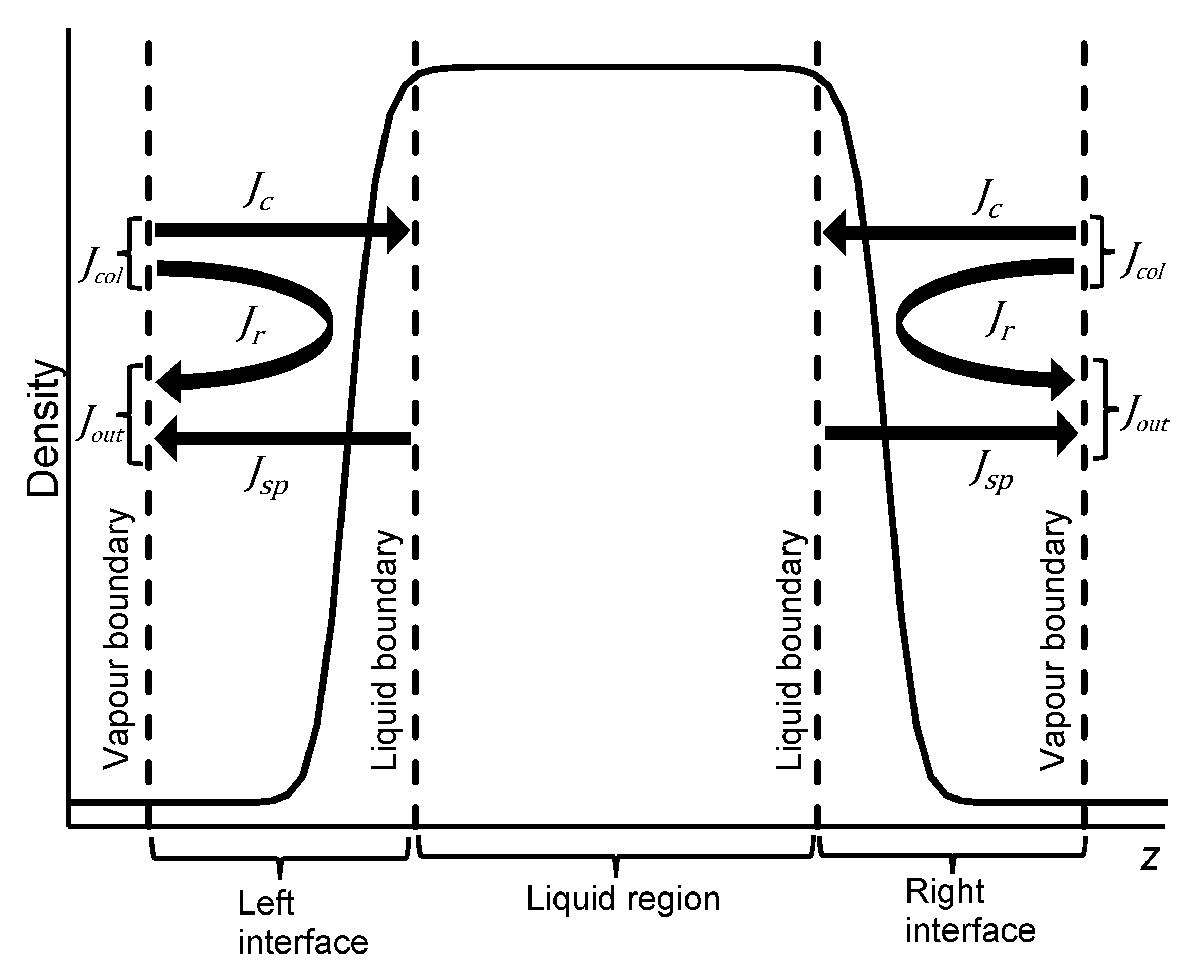
2.1. Liquid-Vapor Phase Equilibria Simulation

The phase equilibria simulation of argon is performed by placing a condensed liquid film in a simulation box with a prolonged length in the z direction and the periodic boundary conditions applied in all three spatial directions. The liquid-vapor equilibria condition is achieved by equilibrating the system at the desired temperature while the initially unoccupied free volume is saturated by the evaporated atoms as the simulation evolves in time. The simulation snapshot is shown in Figure 2.

The positions of the liquid and vapor boundaries were set in terms of the density profile obtained from the production run of the equilibria simulation as shown in Figure 1. The simulation data shows that the density continuously decreases from the liquid phase density to the vapor phase density in the left- and right-side transition regions of the phase equilibria simulation density profile. The transition region density can be well approximated by a hyperbolic tangent function for the left-side interface [29]:

$${\rho }_{le}\left(z\right)=\frac{1}{2}\left({\rho }_v+{\rho }_l\right)-\frac{1}{2}\left({\rho }_v-{\rho }_l\right)tanh\left(\frac{z-z_{0,low}}{{\delta }_{low}}\right)$$

(3)

and for the right-side interface:

$${\rho }_{ri}\left(z\right)=\frac{1}{2}\left({\rho }_v+{\rho }_l\right)+\frac{1}{2}\left({\rho }_v-{\rho }_l\right)tanh\left(\frac{z-z_{0,up }}{{\delta }_{up}}\right)$$

(4)

Here, ${\rho }_l=1275.8 \mathrm{kg}/{\mathrm{m}}^3$ is the simulation liquid phase density, ${\rho }_v=20.9 \mathrm{kg}/{\mathrm{m}}^3$ is the simulation vapor phase density, $z$ is the absolute coordinate in the z axis, $z_0$ is the center position of the density transition region, and $\delta$ is the measure of the transition region thickness. Subscripts le and ri denote the left- and right-side interfaces, respectively. The transition region thickness $d$, a distance over which the density at the interphase drops from 90% of liquid density to 10% of liquid density, is related to the measure of interphase thickness by relation $d=2.1972\delta$ [31]. The values of the fitted transition region parameters are listed in

Table 1. The values of the fitted transition region parameters for left- and right-side interfaces.

${\mathit{z}}_{0,\mathit{l}\mathit{o}\mathit{w}}, \mathbf{\AA }$	${\mathit{z}}_{0,\mathit{u}\mathit{p}}, \mathbf{\AA }$	${\mathit{\delta }}_{\mathit{l}\mathit{o}\mathit{w}},\mathbf{\AA }$	${\mathit{\delta }}_{\mathit{u}\mathit{p}},\mathbf{\AA }$	$\mathit{d},\mathbf{\AA }$
−36.63	36.64	4.17	4.18	9.11

. With the obtained transition region parameter values, the normalized boundary positions were set according to the previous argon study at 90 K [29]: the liquid boundary position was set to $z^{*}=-0.9$, while the vapor boundary was set to $z^{*}=3$. Here, $z^{*}$ is the normalized coordinate of the density transition region

$$z^{*}=\frac{z-z_0}{d}$$

(5)

The normalized and absolute positions for phase equilibria simulation boundaries (listed in Figure 1) are given in

Table 2. The normalized and absolute simulation boundary positions listed in Figure 1.

	${\mathit{z}}^{*}$	$\mathit{z}, \mathbf{\AA }$
Left vapor boundary	3.0	−64.0
Left liquid boundary	−0.9	−27.5
Right liquid boundary	−0.9	27.5
Right vapor boundary	3.0	64.0

.

The atoms that cross the vapor boundaries in an outward direction in equilibria simulation represent the sum of the spontaneously evaporated atoms and the reflected from the interface atoms, as illustrated in Figure 1. Furthermore, the number of argon atoms that crossed the vapor boundaries $N_{out}\left(t\right)$ is a linear function of time, for which the slope coefficient can be found using the linear regression analysis and used to evaluate the outward mass flux [32]:

$$J_{out}=\frac{m_{Ar}b}{S}$$

(6)

Here, $m_{Ar}$ is the mass of an argon atom, $b$ is the slope coefficient of function $N_{out}\left(t\right)$, and $S=2S_{xy}$ is the surface area of total interface region. The outgoing atom mass flux estimated from the phase equilibria simulation is $J_{out}=105.9$ gcm⁻²s⁻¹).

2.2. Deletion Vacuum Simulation

In order to compare the temperature profiles from the vacuum simulations and the equilibrium simulation, a virtual vacuum simulation using a standard approach is performed. In such simulations, the periodic boundary conditions are applied only in x and y, while the vacuum condition near the liquid surfaces is achieved by deleting the atoms that cross the left- and right-side vapor boundaries in an outward direction (thus, this method is regarded as the deletion method throughout this paper). Since there are no incoming atoms from the vapor boundary side, the mass flux crossing the vapor boundary consists only of the spontaneously evaporated atoms as shown in Figure 3. In addition, the vapor and liquid boundaries of the left- and right-side interfaces move along with the depleting liquid film, and the boundary positions are functionals of time [32]:

$$z\left(N_{sp}\left(t\right)\right)=z_0\pm \frac{\left(N_0-N_{sp}\left(t\right)\right)m}{2S_{xy}{\rho }_l}$$

(7)

where $z$ is the boundary position, $N_{sp}\left(t\right)$ is the number of evaporated atoms over time $t$, and $N_0$ is the initial number of atoms. The left side interface boundaries move in a positive z direction, while the right-side interface boundaries move in a negative z direction.

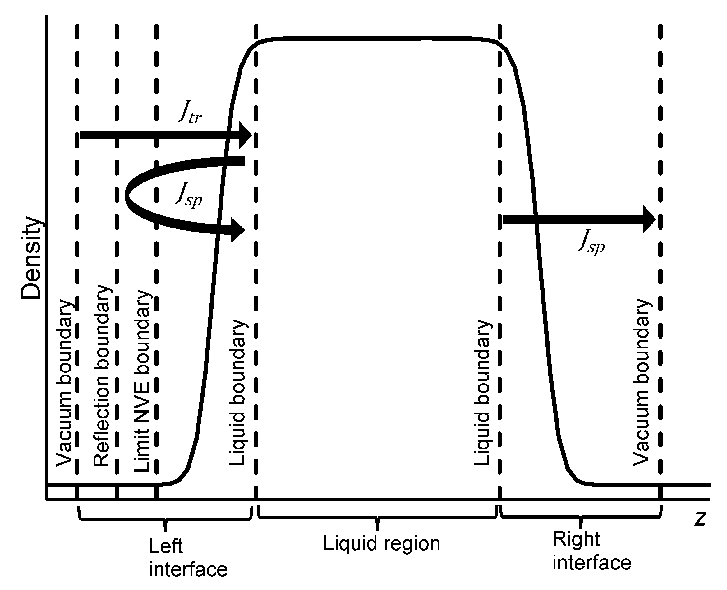
2.3. Steady-State Vacuum Simulation

The technique to simulate the steady-state evaporation/condensation by maintaining the temperature gradient within the liquid film placed in the periodic box was proposed by [33]. In contrast, we propose a simulation approach to simulate the steady-state evaporation process into virtual vacuum by maintaining a constant number of atoms within the liquid film during the simulations. As in case of deletion vacuum simulation, the periodic boundary conditions are applied only in x and y directions. The atoms at the left- and right-side interfaces are managed in the following way (see Figure 4). The right-side interface atoms that cross the vapor boundary are considered as evaporated, and their information (position, speed etc.) is registered. The evaporated atoms are immediately transported to the left-side vapor boundary position (without changing any attribute of the atom except for the position in z axis), thus, creating the virtual vacuum condition near the right-side liquid surface. Then, the evaporated and transported atoms form the mass flux $J_{tr}=J_{sp}$, which replenish the liquid phase from the left-side of the liquid film, thus, maintaining the number of atoms within the liquid film constant. The transportation of the evaporated atoms slightly shifts the center of mass of the system after each evaporation; therefore, the system is recentered to the initial center of mass position every simulation timestep without changing any relative positions or velocities between the atoms to compensate for the center of mass shift.

The transportation of evaporated atoms creates a problem with possible atom overlapping near the left-side vapor boundary. This problem is solved in the following way. The mirror reflection boundary is placed near the left-side vapor boundary as shown in Figure 4. Thus, the spontaneously evaporated atoms from the left-side liquid surface are reflected to the liquid phase after the collisions with the incoming transported atoms or the reflection boundary, and the volume near the left-side vapor boundary is left empty of the interface atoms. However, the overlapping of the short-range repulsion force occurs every 0.22 ns in the volume beyond the reflection boundary when newly evaporated atoms are transported on top of the previously evaporated atoms. Therefore, the dynamics of the atoms in the limit NVE region is solved in the NVE ensemble with the velocity limit, which is allowed for atoms to reach in this region. The velocity limit dissipates the potential energy to a certain value when it is converted to kinetic energy during the interactions between the overlapped atoms. The velocity limit of 800 m/s set in our simulations affects only the highly overlapped atoms due to transportation, while the dynamics of regular atom collisions in the region is solved in the unaltered NVE ensemble. This way, each overlap in the limit NVE region does not break the simulation but rather results in slight growth of the total kinetic energy, which is later accounted for with the thermostat applied to the liquid region. The normalized and absolute positions for steady-state vacuum simulation boundaries (listed in Figure 4) are given in

Table 3. The normalized and absolute simulation boundary positions listed in Figure 4.

	${\mathit{z}}^{*}$	$\mathit{z}, \mathbf{\AA }$
Left vapor boundary	3.0	−64.0
Reflection boundary	2.58	−60.2
Limit NVE boundary	2.16	−56.3
Left liquid boundary	−0.9	−27.5
Right liquid boundary	−0.9	27.5
Right vapor boundary	3.0	64.0

. In addition, the spontaneous evaporation rates $J_{sp}$ in all vacuum simulations were obtained in the same way as the mass flux $J_{out}$ in the phase equilibria simulation (see Equation (6)).

Let us note that, although the evaporation takes place only from the right-side surface, the proposed approach has advantage over the standard deletion virtual vacuum simulation method, since one can carry out simulations at desired evaporation states for arbitrary amounts of time and collect sufficient statistical data for that state rather than being limited to short period of time, during which the system can be regarded as quasi-steady.

2.4. Net Momenum in Steady-State Vacuum Simulation

The net momentum problem resulting from evaporated atom transportation needs to be addressed as it is related to the accuracy and the correctness of the proposed method. The transportation of evaporated atoms introduces net momentum changes in the system $\Delta p_z$, which consequently induces the force acting on the liquid phase in the z direction. This force is proportional to the momentum change $\Delta p_z$ and can be approximately evaluated in the following way:

$$F_z=m{a}_z=\frac{\Delta p_z}{\Delta t}=\frac{\mathsf{\Delta }m·v_z}{\Delta t}\approx \frac{m_{Ar}\Delta N_{sp}{\overline{v}}_z}{\Delta t}=m_{Ar}{J}_{sp}{S}_{xy}{\overline{v}}_z$$

(8)

where $\Delta p_z$ is the momentum change over time $\Delta t$, $\mathsf{\Delta }m$ is the transporter mass over time $\Delta t$, $v_z$ is the velocity in z direction, $\Delta N_{sp}$ is the number of spontaneously evaporated atoms at the right vapor boundary over time $\Delta t$, ${\overline{v}}_z$ is the average velocity of evaporated atoms in the z direction. Furthermore, the atoms evaporated to the left side are reflected by the mirror reflection boundary back to the liquid, thus also inducing the momentum change, which induces the force on the liquid phase equal to $2m_{Ar}{J}_{sp}{S}_{xy}{\overline{v}}_z$ (assuming that all evaporated atoms were reflected by the boundary). However, a fraction of the atoms is reflected by the collisions with the incoming transported atoms; therefore, the total force acting on the liquid phase $F_z$ is expect to be in the interval of $\left[m_{Ar}{J}_{sp}{S}_{xy}{\overline{v}}_z; 3m_{Ar}{J}_{sp}{S}_{xy}{\overline{v}}_z\right]$. This force accelerates only the liquid phase, or, in our case, decelerates the evaporated atoms at the right-side interface with rate:

$$a_z=\frac{F_z}{m_{liq}}\approx \frac{F_z}{N{m}_{Ar}}$$

(9)

when the center of mass velocity is subtracted from every atom of the system every simulation timestep to keep the liquid phase velocity at zero. Here, $N$ is the total number of argon atoms in the system. As a result, the energetic characteristics of the collected ensemble of evaporated atoms in the z direction should be shifted to the lower energy side. However, the velocity deceleration of the evaporated atoms is negligible over the time periods it takes for the atoms to travel from the liquid surface to the vapor boundary. For example, the evaporated atom with an average velocity ${\overline{v}}_z=171.53$ m/s is decelerated by negligible the amount of 0.31 m/s (or 0.18% of the initial value) by the time the atom travels the distance from the liquid surface to the right vapor boundary ($l_{evap}=28.04$ Å) with the representative spontaneous evaporation rate $J_{sp}=5.67\times {10}^{27}$ × 1/m²s and the upper estimation of the deceleration rate $a_z=1.91\times {10}^{10}$ m/s². Consequently, the results show that no noticeable velocity distribution shifts were observed for evaporating atoms compared to the Maxwellian distribution at 90 K. The average velocity of evaporated atoms at 90 K was estimated assuming the Maxwellian distribution in the evaporated atoms [32]:

$${\overline{v}}_z=\sqrt{\frac{\pi k_{B}T}{2m_{Ar}}}$$

(10)

Furthermore, the method error is expected to scale with the increasing simulation temperature since the spontaneous evaporation rate $J_{sp}$ is an increasing function of temperature. Therefore, the deceleration rates and corresponding errors should be evaluated before analyzing the statistics of evaporated atoms at higher temperature simulations.

2.5. Simulation Details

Argon phase equilibria and evaporation simulations were performed by initially placing the condensed liquid film (consisting of 18,000 argon atoms) in a simulation box prolonged in the z direction. The box dimensions for the phase equilibria and all the vacuum simulations were 108.6 × 108.6 × 443.1 Å and 108.6 × 108.6 × 140 Å, respectively. The interaction between argon atoms was described using Lennard-Jones (LJ) potential [24]:

$$U\left(r_{ij}\right)=4\epsilon \left[{\left(\frac{\sigma }{r_{ij}}\right)}^{12}-{\left(\frac{\sigma }{r_{ij}}\right)}^6\right]$$

(11)

where $\epsilon$ is the depth of the (LJ) potential well, $\sigma$ is the interaction length parameter, and $r_{ij}$ is the distance between i and j atoms. LJ interaction parameter values used for argon are $\sigma =3.405$ Å and $\epsilon /k_B=119.8$ K. The cut-off distance used in simulations was $3\sigma$. The Newtonian equations of motion of system atoms were solved using the Verlet method with an integration timestep value of Δt = 4 fs. The simulation data output was performed every 200 timesteps while gathering the information on evaporated atoms.

In all simulations, the system was equilibrated at 90 K before the production run started. In the phase equilibria simulation, the system was equilibrated for 2 ns with the thermostat applied to the whole domain. Then, the production run was performed in the NVE ensemble for 50 ns. In the deletion vacuum simulation, the thermostat was applied only to the volume between the thermostat region boundaries, which were set in the same position as the liquid boundaries during the whole simulation length. Meanwhile, the interface atoms were simulated in the NVE ensemble. The system was equilibrated for only 0.2 ns before the production run because of the limited time before the liquid film depletes. The production run lasted until the number of argon atoms in the system decreased to 10,000. In the case of the steady-state vacuum simulations, the system was equilibrated for 2 ns before the 200 ns production run. The investigated temperature control strategies for the steady-state vacuum simulations are described in the following sections. The thermostat algorithm of choice was the Nosé–Hoover thermostat, which maintains the targeted temperature in the system (or the specific parts of the system) by adding a force term to the Newtonian equations of motion [34].

Unlike in the steady-state vacuum and phase equilibria simulations, in which the profiles were averaged over the whole production run, the temporal temperature profiles presented from the deletion vacuum simulation were averaged over every 40 ps periods due to interface movement of the evaporating film. Furthermore, the temperature profiles were calculated by subtracting the flow velocity of each bin from all atoms within the bin. All the simulations in this paper were performed using LAMMPS molecular dynamics code [35].

3. Results and Discussion

3.1. Temperature Profile in Virtual Vacuum Simulation

We begin this section by comparing the phase equilibria simulation temperature profile with the temperature profiles from the deletion vacuum and our proposed steady-state vacuum simulations. In both vacuum simulations, the standard temperature control scheme is used where the interface regions are simulated in the NVE ensemble, and the simulation temperature is maintained with the thermostat applied to the thermostat region, which coincides with the liquid phase [24,26,27,28,29]. The reason for the thermostat region boundaries being set below the liquid surface position is that the thermostat would not affect the evaporating atoms in the interface. The temperature profiles of all three simulations are given in Figure 5. In the phase equilibria simulation, the temperature is uniform in all regions of the simulation since the net heat and mass fluxes are zero at the liquid surfaces. Meanwhile, the temperature profiles in the vacuum simulations are non-uniform in both the liquid and interface regions. In case of the deletion vacuum simulation, the liquid region possesses a parabolic temperature profile form with temperature values above 90 K in the middle of the liquid, and the temperature values below 90 K at the liquid surface position located around coordinate $z^{*}=0$ [14]. The parabolic shape in the liquid phase is caused by the combination of the evaporative heat sink effect, which lowers the temperature of the liquid surfaces, and the heat source in the liquid phase, which is induced by the thermostat maintaining the average simulation temperature within the thermostat region boundaries. The same temperature control approach in the constant vacuum state simulation leads to a similar problem: the temperature has a decreasing linear shape in the liquid region, which is caused by the heat sink at the right-side surface and heat source at the left-side surface due to incoming transported atoms. In both vacuum simulation cases, the temperature drops rapidly beyond the evaporating liquid surfaces because part of the thermal energy of evaporated atoms is converted to the kinetic energy of the macroscopic evaporation flow in the z axis [36]. Let us also note that the temperature profile from the constant vacuum state simulation is considerably smoothened by the greater amount of collected statistical data compared to the deletion vacuum simulation profile, in which violent fluctuations are present, especially in the interface.

The comparison of temperature profiles in the liquid phase and near the liquid surface (as shown in Figure 5) clearly demonstrates the problem related with the commonly used temperature control approach: the spontaneous evaporation rates used to evaluate the evaporation coefficients from the phase equilibria simulations are obtained at lower surface temperatures in the virtual vacuum simulations compared to the surface temperatures in the phase equilibria simulations. Such temperature differences introduce errors in the evaporation coefficient evaluation from the perspective of molecular dynamics simulations, especially at higher temperatures where the evaporation rates scale exponentially with temperature. Hence, the following sections are focused on the vacuum simulation temperature control strategies to maintain the uniform temperature profile across the liquid phase, the errors induced by the surface temperature differences on the estimation of spontaneous evaporation rates and corresponding evaporation coefficients, and the thermostat impact on the energetic characteristics of the evaporating atoms.

3.2. Spontaneous Evaporation Rate Dependency on Surface Temperature

To deal with the non-uniform temperature profile in the liquid phase, the thermostat region was divided into several bins with varying bin width, and the thermostat was applied to each bin separately to maintain the average desired temperature within each bin. The simulations were performed with different bin widths of 27.5, 18.4, 9.2, 6.1, and 3.1 Å, which correspond to 2, 3, 6, 9, and 18 division bins in the liquid region, respectively. The temperature profiles shown in Figure 6 demonstrate that dividing the liquid phase into 2 bins with bin widths of 27.5 Å already makes the temperature profile flatter in the liquid phase, and the temperature at the surface is increased to 88.7 K compared to 87.55 K obtained in the one bin case (no division). However, Figure 6b shows that the further division into thinner bins is not as effective and has little impact on the surface temperature because the temperatures at the surface position group below desired temperature of 90 K in all bin width cases. Consequently, the division into 2 bins leads to increased spontaneous evaporation rates, with the evaporation coefficient values increasing by 11%, as shown in Figure 7, while the spontaneous evaporation rate increases by another 2.5% and reaches saturation value when bin size is reduced to 9.2 Å.

Since the energy is drawn from the liquid surface due to the evaporative heat sink, the evaporating surface temperature depends on the separation distance, through which the heat is conducted from the liquid film to the surface, i.e., the distance between the surface and the thermostat region boundaries. Thus, the temperature of the evaporating surface is below the desired temperature by several K with the separation distance of 27.5 Å (above cases), even when the liquid phase is divided into separately thermostated bins, which level out the temperature profiles in the liquid phase. Since there are no objective criteria to define the liquid phase and thermostat region boundary positions, we performed simulations with different thermostat region boundary positions at the right-side interface. The thermostat region boundary position of the left-side interface was set to $z^{*}=-0.9$ as in previous cases, and the number of thermostated bins were set to 6. The obtained temperature profiles are shown in Figure 8. As expected, the temperature profiles show that the liquid surface temperature in the vacuum simulations linearly increases from 88.31 K to 90 K when the thermostat region boundary position at the right-side interface changes from −2 to +1. Furthermore, Figure 8 demonstrates that the liquid surface temperature can be maintained at the desired temperature of 90 K only when the thermostat region boundary is placed beyond the liquid surface position, i.e., at position +1. At this point, the heat is induced by the thermostat directly to the liquid surface to compensate for the heat sink effect as if the thermal energy was conducted from the liquid phase to the surface infinitely fast.

The varying liquid surface temperature and the spontaneous evaporation rate with changing thermostat region boundary position provide a possibility to investigate the correlation between these two quantities. The results given in Figure 9a show that the spontaneous evaporation rate can be approximated as an increasing linear function of the liquid surface temperature in a given temperature range. Furthermore, the spontaneous evaporation rate decreases from 64.48 to 50.93 ${\mathrm{gcm}}^{-2}{\mathrm{s}}^{-1}$ as the liquid surface temperature drops from the targeted value of 90 K to 87.55 K. This example illustrates the sensitivity of the evaporation rate to the chosen temperature control approach and small changes of liquid surface temperature in virtual vacuum simulations. As a result, the evaporation coefficient value estimated from the MD simulations can be influenced by more than 21% with the relatively small deviations of liquid surface temperature from the targeted temperature, as illustrated in Figure 9b. Such small temperature deviations might have an even greater impact on the evaporation coefficient estimation at the higher temperatures as the evaporation rate is an exponential function of the temperature.

3.3. Velocity Distributions of Evaporating Atoms

Although the thermostat region boundary position at the right-side interface affects the liquid surface temperature and, in turn, the spontaneous evaporation rate, it has little to no effect on the average kinetic energy components of evaporating argon atoms in x and y directions, as shown in Figure 10. A slight increase of the average kinetic energy component in the z direction can be seen when the thermostat region boundary position changes in the investigated range; however, the increase is less than 3%. The velocity distribution functions given in Figure 11 also show that the thermostat region boundary position has little to no noticeable impact on the velocity distributions of evaporating argon atoms in all three spatial directions. The simulation velocity distribution functions in the z direction are slightly shifted to the right side in all thermostat boundary position cases with the mean velocity component values greater by $3.74 \mathrm{m}/\mathrm{s}$ on average than the Maxwellian distribution average ${\overline{v}}_{z,Maxw}=171.5 \mathrm{m}/\mathrm{s}$ at 90 K. Furthermore, the unchanged velocity distribution functions demonstrate that although the thermostat region boundary position is placed beyond the liquid surface position, the thermostat itself does not alter the dynamics of evaporating atoms at the interface in any meaningful way. This is because the last bin of the thermostat region contains not only the evaporating argon atoms at the interface but also a considerable amount of liquid atoms near the liquid surface. Therefore, there is no need for the thermostat algorithm to do significant alterations in the individual atom dynamics to maintain a constant temperature within the bin ensemble.

4. Conclusions

In the present paper, a constant virtual vacuum state simulation method was proposed, in which the virtual vacuum condition is achieved at the right-side interface by transporting the evaporated atoms to the left-side vapor boundary and recentering the systems center of mass at each timestep to adjust for the transportation effects. The proposed method was used to perform virtual vacuum simulations of argon at 90 K in order to study the effects of the chosen temperature control approach in virtual vacuum simulations on the system’s temperature profiles, spontaneous evaporation rates and corresponding evaporation coefficient values, and the energetic characteristics of the evaporated atoms. The following conclusions can be made from the results presented in this study:

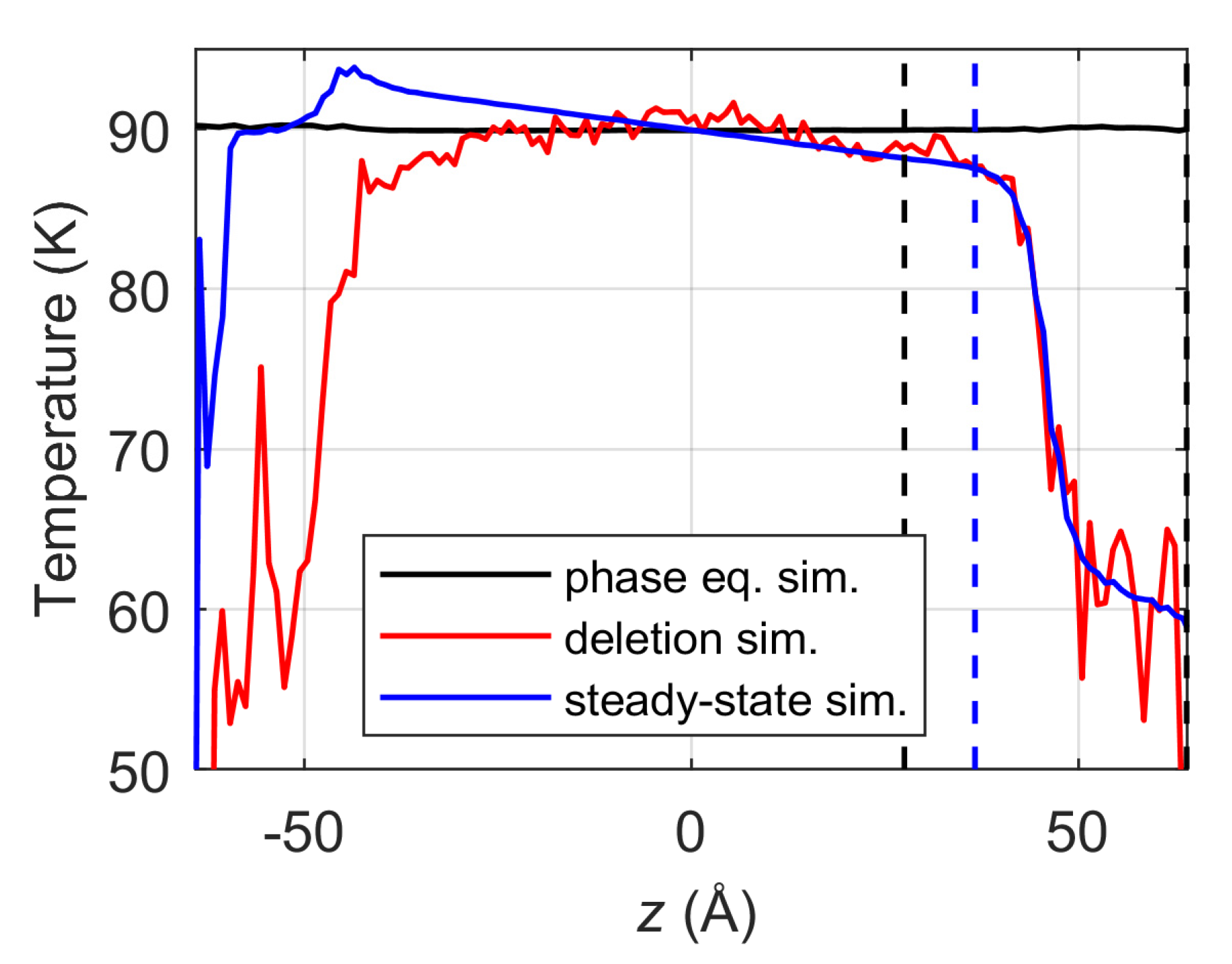
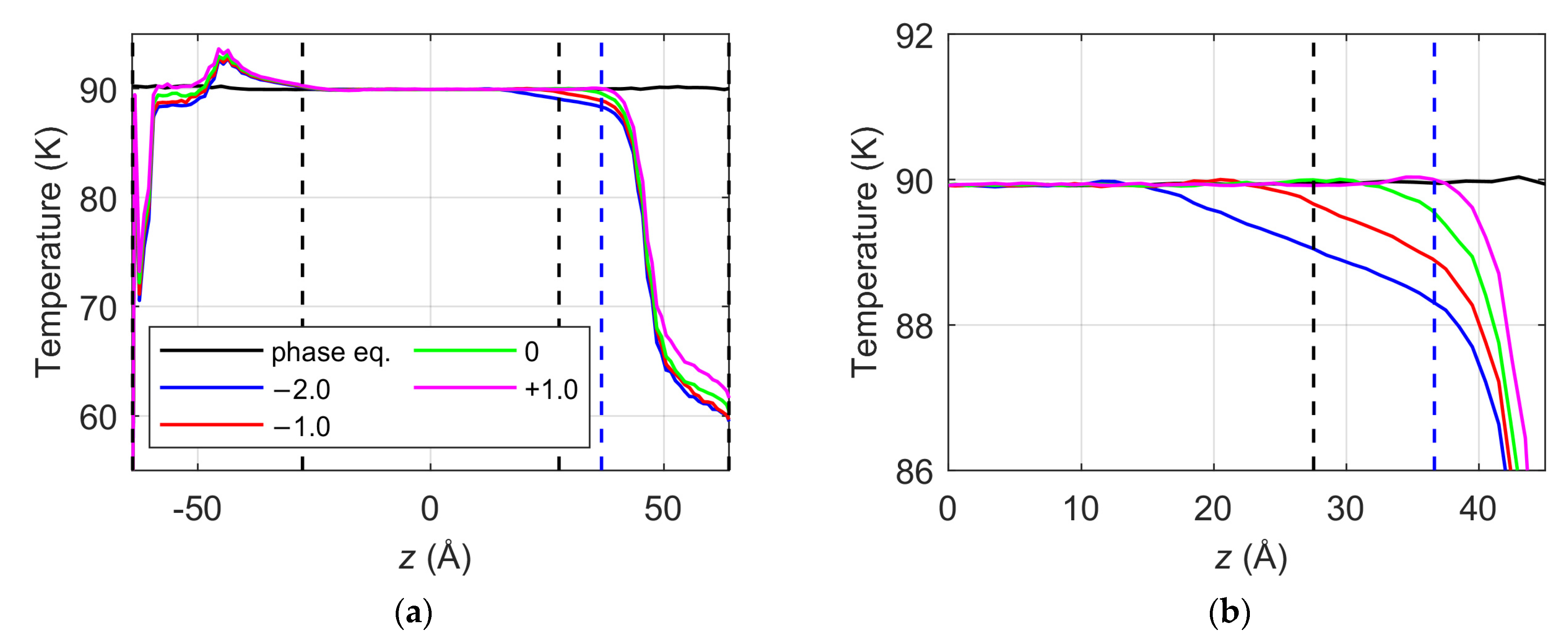
• In both the deletion vacuum and the steady-state vacuum simulations, the temperature control approach, in which the thermostat is simply applied only to the liquid phase and the interfaces are simulated in the NVE ensemble, provides non-uniform parabolic temperature profiles across the liquid phase due to the evaporative heat sink at the evaporating surface. Consequently, the temperature at the liquid surface position is obtained lower by several K compared to the targeted simulation temperature of 90 K.
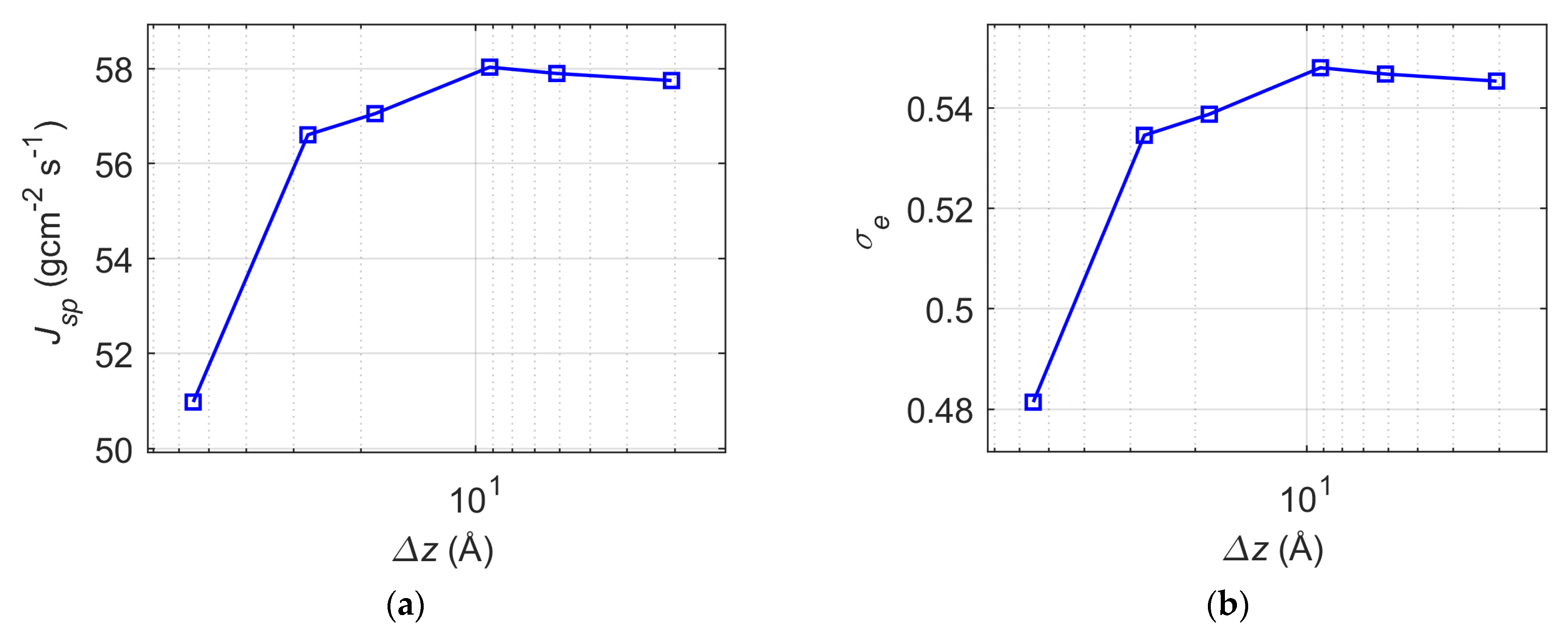
• In steady-state vacuum simulations, the division of the liquid phase into 2 bins, to which the thermostat is applied separately, already flattens the non-uniform temperature profiles and raises the liquid surface temperature; however, the surface temperature reaches saturation value below the targeted temperature with the further reduction of bin width below 9.2 Å. Consequently, the division into 2 bins leads to increased spontaneous evaporation rates, with the evaporation coefficient values increasing by 11%, and the spontaneous evaporation rate increases by another 2.5% and reaches saturation value when bin width is reduced to 9.2 Å.
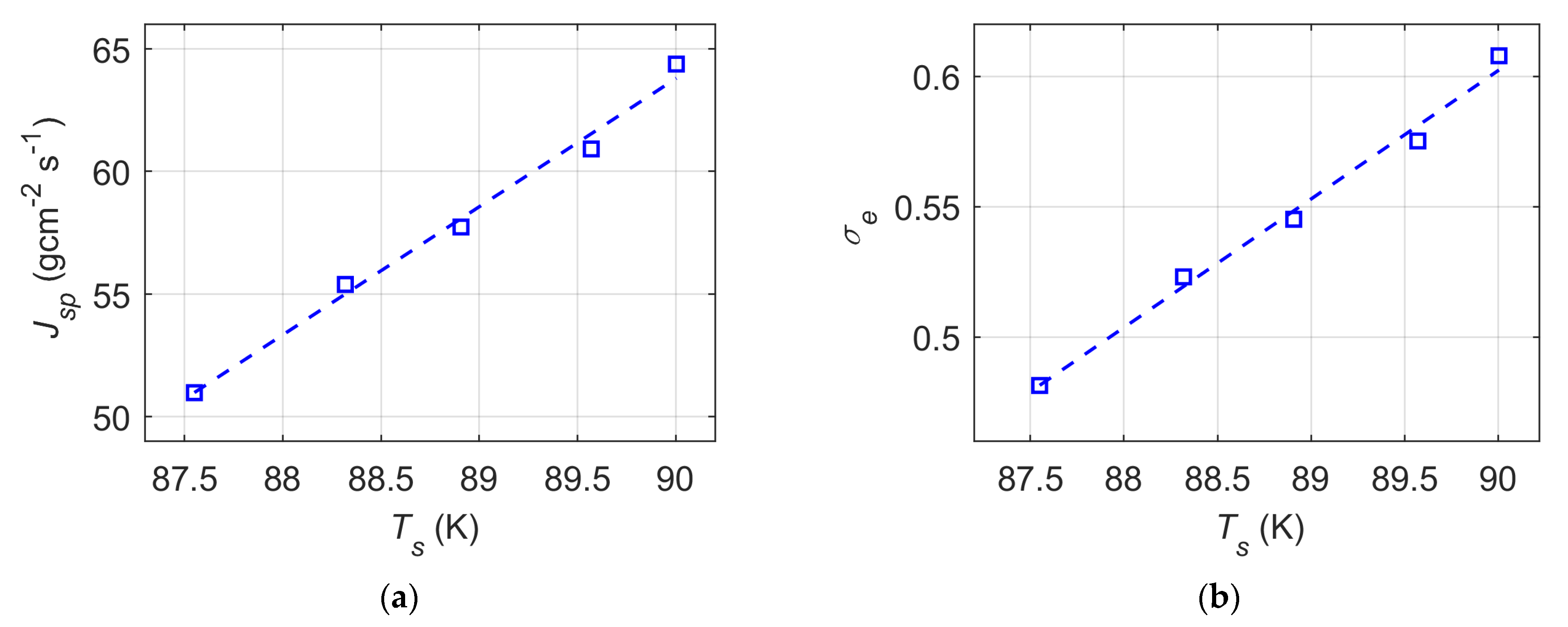
• The liquid surface temperature increases linearly with increasing normalized (or absolute) thermostat region boundary position values at the right-side interface; however, the surface temperature reaches the targeted simulation temperature of 90 K only when the thermostat boundary is placed beyond the liquid surface. Furthermore, the spontaneous evaporation rate is an increasing linear function of the liquid surface temperature in a temperature range of 87.55–90 K. In this narrow range, the spontaneous evaporation rate and corresponding evaporation coefficient estimation from MD simulations can vary up to 21%.
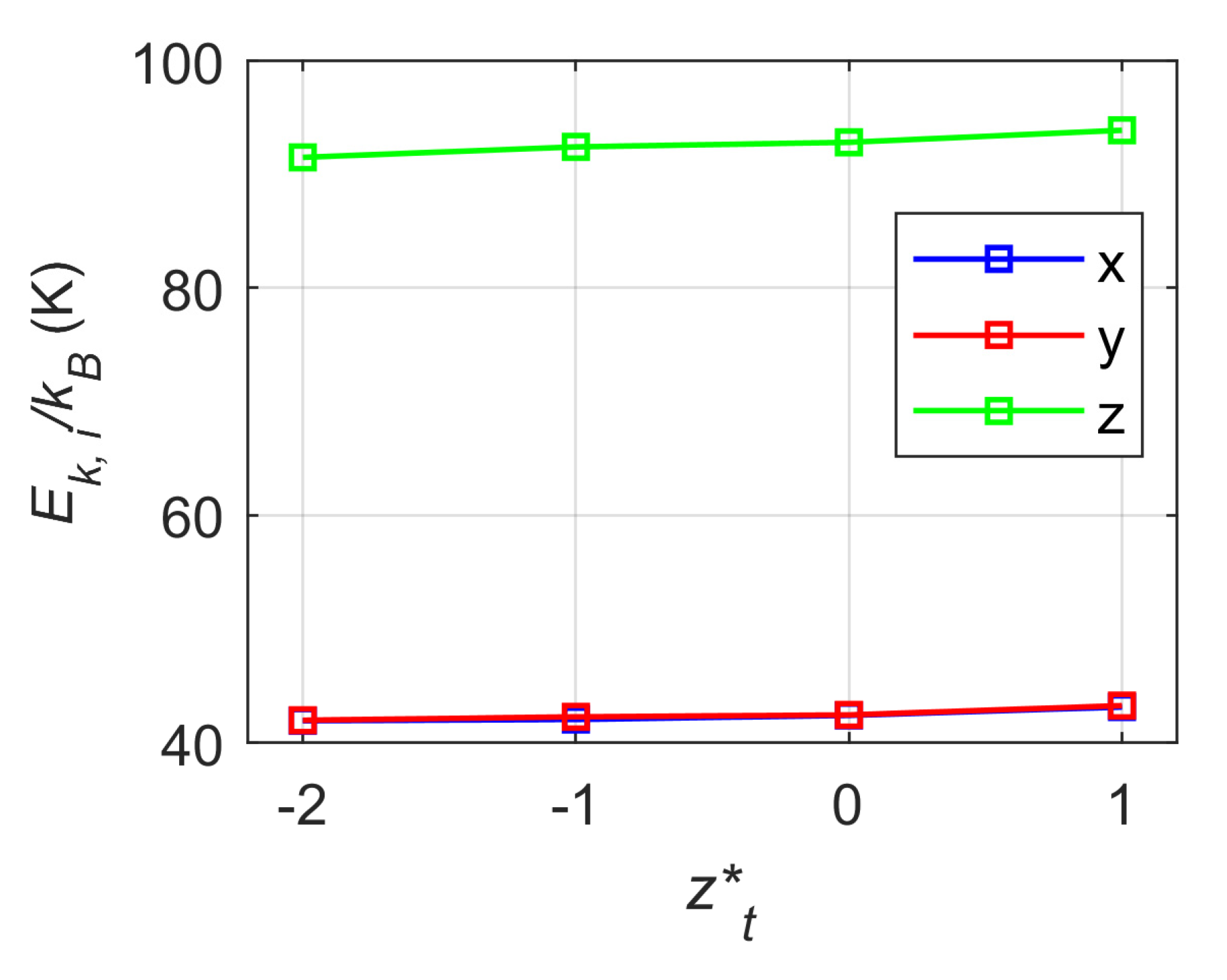
• The velocity distributions of evaporating argon atoms in x, y and z directions follow the Maxwellian distribution for all simulated cases, and the thermostat has little to no noticeable effect on the energy characteristics and velocity distributions of the evaporating argon atoms, even when the thermostat boundary is placed above the liquid surface.
• The proposed temperature control strategies can be used to obtain the evaporation/condensation coefficient values at desired liquid surface temperatures in practical applications.

References

1. Tas, N.R.; Mela, P.; Kramer, T.; Berenschot, J.W.; Van Den Berg, A. Capillarity Induced Negative Pressure of Water Plugs in Nanochannels. Nano Lett. 2003, 3, 1537–1540. [Google Scholar] [CrossRef] [Green Version]
2. Duan, C.; Karnik, R.; Lu, M.C.; Majumdar, A. Evaporation-induced cavitation in nanofluidic channels. Proc. Natl. Acad. Sci. USA 2012, 109, 3688–3693. [Google Scholar] [CrossRef] [PubMed] [Green Version]
3. Ajeel, R.K.; Salim, W.S.I.W.; Hasnan, K. Design characteristics of symmetrical semicircle-corrugated channel on heat transfer enhancement with nanofluid. Int. J. Mech. Sci. 2019, 151, 236–250. [Google Scholar] [CrossRef]
4. Ajeel, R.K.; Zulkifli, R.; Sopian, K.; Fayyadh, S.N.; Fazlizan, A.; Ibrahim, A. Numerical investigation of binary hybrid nanofluid in new configurations for curved-corrugated channel by thermal-hydraulic performance method. Powder Technol. 2021, 385, 144–159. [Google Scholar] [CrossRef]
5. Ajeel, R.K.; Sopian, K.; Zulkifli, R. A novel curved-corrugated channel model: Thermal-hydraulic performance and design parameters with nanofluid. Int. Commun. Heat Mass Transf. 2021, 120, 105037. [Google Scholar] [CrossRef]
6. Baghbanzadeh, M.; Lan, C.Q.; Rana, D.; Matsuura, T. Membrane Distillation. J. Memb. Sci. 1997, 1, 419–455. [Google Scholar] [CrossRef]
7. Lee, J.; Karnik, R. Desalination of water by vapor-phase transport through hydrophobic nanopores. J. Appl. Phys. 2010, 108, 044315. [Google Scholar] [CrossRef]
8. Skarbalius, G.; Džiugys, A.; Misiulis, E.; Navakas, R.; Vilkinis, P.; Šereika, J.; Pedišius, N. Molecular dynamics study on water flow behaviour inside planar nanochannel using different temperature control strategies. Energies 2021, 14, 6843. [Google Scholar] [CrossRef]
9. Cailliez, F.; Stirnemann, G.; Boutin, A.; Demachy, I.; Fuchs, A.H. Does water condense in hydrophobic cavities? A molecular simulation study of hydration in heterogeneous nanopores. J. Phys. Chem. C 2008, 112, 10435–10445. [Google Scholar] [CrossRef]
10. Wu, X.; Yang, Z.; Duan, Y. Molecular dynamics simulation on evaporation of a suspending difluoromethane nanodroplet. Int. J. Heat Mass Transf. 2020, 158, 120024. [Google Scholar] [CrossRef]
11. James, M.; Darwish, T.A.; Ciampi, S.; Sylvester, S.O.; Zhang, Z.; Ng, A.; Gooding, J.J.; Hanley, T.L. Nanoscale condensation of water on self-assembled monolayers. Soft Matter 2011, 7, 5309–5318. [Google Scholar] [CrossRef] [Green Version]
12. Persad, A.H.; Ward, C.A. Expressions for the Evaporation and Condensation Coefficients in the Hertz-Knudsen Relation. Chem. Rev. 2016, 116, 7727–7767. [Google Scholar] [CrossRef] [PubMed]
13. Hołyst, R.; Litniewski, M.; Jakubczyk, D. A molecular dynamics test of the Hertz-Knudsen equation for evaporating liquids. Soft Matter 2015, 11, 7201–7206. [Google Scholar] [CrossRef] [PubMed]
14. Liang, Z.; Biben, T.; Keblinski, P. Molecular simulation of steady-state evaporation and condensation: Validity of the Schrage relationships. Int. J. Heat Mass Transf. 2017, 114, 105–114. [Google Scholar] [CrossRef]
15. Barnes, G.T. The effects of monolayers on the evaporation of liquids. Adv. Colloid Interface Sci. 1986, 25, 89–200. [Google Scholar] [CrossRef]
16. Mozurkewich, M. Aerosol growth and the condensation coefficient for water: A review. Aerosol Sci. Technol. 1986, 5, 223–236. [Google Scholar] [CrossRef]
17. Marek, R.; Straub, J. Analysis of the evaporation coefficient and the condensation coefficient of water. Int. J. Heat Mass Transf. 2001, 44, 39–53. [Google Scholar] [CrossRef]
18. Davis, E.J. A history and state-of-the-art of accommodation coefficients. Atmos. Res. 2006, 82, 561–578. [Google Scholar] [CrossRef]
19. Badam, V.K.; Kumar, V.; Durst, F.; Danov, K. Experimental and theoretical investigations on interfacial temperature jumps during evaporation. Exp. Therm. Fluid Sci. 2007, 32, 276–292. [Google Scholar] [CrossRef]
20. Gatapova, E.Y.; Graur, I.A.; Kabov, O.A.; Aniskin, V.M.; Filipenko, M.A.; Sharipov, F.; Tadrist, L. The temperature jump at water—Air interface during evaporation. Int. J. Heat Mass Transf. 2017, 104, 800–812. [Google Scholar] [CrossRef]
21. Rokoni, A.; Sun, Y. Probing the temperature profile across a liquid-vapor interface upon phase change. J. Chem. Phys. 2020, 153, 144706. [Google Scholar] [CrossRef] [PubMed]
22. Bird, E.; Liang, Z. Transport phenomena in the Knudsen layer near an evaporating surface. Phys. Rev. E 2019, 100, 43108. [Google Scholar] [CrossRef] [PubMed]
23. Cheng, S.; Lechman, J.B.; Plimpton, S.J.; Grest, G.S. Evaporation of Lennard-Jones fluids. J. Chem. Phys. 2011, 134, 224704. [Google Scholar] [CrossRef] [PubMed] [Green Version]
24. Ishiyama, T.; Yano, T.; Fujikawa, S. Molecular dynamics study of kinetic boundary condition at an interface between argon vapor and its condensed phase. Phys. Fluids 2004, 16, 2899. [Google Scholar] [CrossRef] [Green Version]
25. Xie, J.F.; Sazhin, S.S.; Cao, B.Y. Molecular dynamics study of the processes in the vicinity of the n-dodecane vapour/liquid interface. Phys. Fluids 2011, 23, 1–12. [Google Scholar] [CrossRef] [Green Version]
26. Ishiyama, T.; Yano, T.; Fujikawa, S. Molecular dynamics study of kinetic boundary condition at an interface between a polyatomic vapor and its condensed phase. Phys. Fluids 2004, 16, 4713–4727. [Google Scholar] [CrossRef]
27. Ishiyama, T.; Fujikawa, S.; Kurz, T.; Lauterborn, W. Nonequilibrium kinetic boundary condition at the vapor-liquid interface of argon. Phys. Rev. E—Stat. Nonlinear Soft Matter Phys. 2013, 88, 042406. [Google Scholar] [CrossRef] [PubMed]
28. Kobayashi, K.; Hori, K.; Yaguchi, H.; Watanabe, M. Molecular dynamics simulation on evaporation molecules in a vapor-liquid equilibrium state. Proc. 29th Int. Symp. Rarefied Gas Dyn. 2014, 1628, 404–410. [Google Scholar] [CrossRef]
29. Kobayashi, K.; Hori, K.; Kon, M.; Sasaki, K.; Watanabe, M. Molecular dynamics study on evaporation and reflection of monatomic molecules to construct kinetic boundary condition in vapor—Liquid equilibria. Heat Mass Transf. 2015, 52, 1851–1859. [Google Scholar] [CrossRef] [Green Version]
30. Bird, E.; Gutierrez Plascencia, J.; Keblinski, P.; Liang, Z. Molecular simulation of steady-state evaporation and condensation of water in air. Int. J. Heat Mass Transf. 2022, 184, 122285. [Google Scholar] [CrossRef]
31. Yang, T.H.; Pan, C. Molecular dynamics simulation of a thin water layer evaporation and evaporation coefficient. Int. J. Heat Mass Transf. 2005, 48, 3516–3526. [Google Scholar] [CrossRef]
32. Skarbalius, G.; Džiugys, A.; Misiulis, E.; Navakas, R. Molecular dynamics study on water evaporation/condensation parameters. Microfluid. Nanofluidics 2021, 25, 81. [Google Scholar] [CrossRef]
33. Zhakhovsky, V.V.; Kryukov, A.P.; Levashov, V.Y.; Shishkova, I.N.; Anisimov, S.I. Mass and heat transfer between evaporation and condensation surfaces: Atomistic simulation and solution of Boltzmann kinetic equation. Proc. Natl. Acad. Sci. USA 2019, 116, 18209–18217. [Google Scholar] [CrossRef] [PubMed] [Green Version]
34. Sam, A.; Kannam, S.K.; Hartkamp, R.; Sathian, S.P. Water flow in carbon nanotubes: The effect of tube flexibility and thermostat. J. Chem. Phys. 2017, 146, 234701. [Google Scholar] [CrossRef] [Green Version]
35. Thompson, A.P.; Aktulga, H.M.; Berger, R.; Bolintineanu, D.S.; Brown, W.M.; Crozier, P.S.; in ’t Veld, P.J.; Kohlmeyer, A.; Moore, S.G.; Nguyen, T.D.; et al. LAMMPS—A flexible simulation tool for particle-based materials modeling at the atomic, meso, and continuum scales. Comput. Phys. Commun. 2022, 271, 108171. [Google Scholar] [CrossRef]
36. Liang, Z.; Chandra, A.; Bird, E.; Keblinski, P. A molecular dynamics study of transient evaporation and condensation. Int. J. Heat Mass Transf. 2020, 149, 119152. [Google Scholar] [CrossRef]
Figure 1. Phase equilibria simulation scheme with denoted interface region boundary positions and mass fluxes through the interfaces. The density profile for the scheme was obtained from the production run of the liquid-vapor phase equilibria simulation.
Applsci 13 00256 g001
Figure 2. Phase equilibria simulation snapshot at a random moment of time. The periodic boundary conditions are applied to x, y and z axes.
Applsci 13 00256 g002
Figure 3. Deletion vacuum simulation scheme with denoted interface region boundary positions and mass fluxes through the interfaces. The density profile for the scheme was obtained from the production run of the liquid-vapor phase equilibria simulation.
Applsci 13 00256 g003
Figure 4. Steady-state vacuum simulation scheme with denoted interface region boundary positions and mass fluxes through the interfaces. The density profile for the scheme was obtained from the production run of the liquid-vapor phase equilibria simulation.
Applsci 13 00256 g004
Figure 5. A phase equilibria simulation temperature profile comparison with the temperature profiles obtained from the deletion vacuum simulation and the steady-state vacuum simulation. The vertical dotted lines represent the liquid/thermostat and vapor boundary positions of the right-side interface, respectively, while the blue dotted line represents the liquid surface position located at coordinate z * = 0 . Note: the deletion vacuum simulation temperature profile is slightly shifted so that the right-side interfaces from all three simulations would coincide.
Applsci 13 00256 g005
Figure 6. (a) The temperature profiles from simulations with different thermostat region division bin widths, and (b) the zoomed view of these profiles in the liquid region near the liquid surface. The black dotted lines denote the liquid/thermostat and vapor boundary positions z * = 0.9 and z * = 3 for both left- and right-side interfaces, while the blue dotted line denote the liquid surface position z * = 0 . For comparison, the temperature profiles from the phase equilibria simulation and the steady-state vacuum simulation with no bin division are also plotted.
Applsci 13 00256 g006
Figure 7. (a) The spontaneous evaporation rate, and (b) the corresponding evaporation coefficient as a function of the liquid phase division bin width in steady-state vacuum simulations. The first point (55 Å bin width) represents the data point for simulations without the liquid phase division.
Applsci 13 00256 g007
Figure 8. (a) The temperature profiles from simulations with different thermostat region boundary positions at the right-side interface, and (b) the zoomed view of these profiles in the liquid region near the liquid surface. The black dotted lines denote the liquid and vapor boundary positions z * = 0.9 and z * = 3 for both left- and right-side interfaces, while the blue dotted line denote the liquid surface position z * = 0 . For comparison, the temperature profile from the phase equilibria simulation is also plotted.
Applsci 13 00256 g008
Figure 9. (a) The spontaneous evaporation rate, and (b) the corresponding evaporation coefficient as functions of liquid surface temperature in steady-state vacuum simulations.
Applsci 13 00256 g009
Figure 10. The average kinetic energy components in x, y, and z axis of evaporating argon atoms as a functions of normalized thermostat boundary position at the right-side interface.
Applsci 13 00256 g010
Figure 11. Velocity distribution functions of evaporating argon atoms at the right-side vapor boundary in (a) x, (b) y and (c) z axes with different thermostat region boundary positions z t * .
Applsci 13 00256 g011