Review

Short Text Clustering Algorithms, Application and Challenges: A Survey

1
CAIT, Faculty of Information Science and Technology, Universiti Kebangsaan Malaysia, Bangi 43600, Selangor, Malaysia
2
Ministry of Higher Education and Scientific Research, Baghdad 10065, Iraq
*
Authors to whom correspondence should be addressed.
Appl. Sci. 2023, 13(1), 342; https://doi.org/10.3390/app13010342
Submission received: 19 October 2022 / Revised: 25 November 2022 / Accepted: 16 December 2022 / Published: 27 December 2022

Abstract

:
The number of online documents has rapidly grown, and with the expansion of the Web, document analysis, or text analysis, has become an essential task for preparing, storing, visualizing and mining documents. The texts generated daily on social media platforms such as Twitter, Instagram and Facebook are vast and unstructured. Most of these generated texts come in the form of short text and need special analysis because short text suffers from lack of information and sparsity. Thus, this topic has attracted growing attention from researchers in the data storing and processing community for knowledge discovery. Short text clustering (STC) has become a critical task for automatically grouping various unlabelled texts into meaningful clusters. STC is a necessary step in many applications, including Twitter personalization, sentiment analysis, spam filtering, customer reviews and many other social network-related applications. In the last few years, the natural-language-processing research community has concentrated on STC and attempted to overcome the problems of sparseness, dimensionality, and lack of information. We comprehensively review various STC approaches proposed in the literature. Providing insights into the technological component should assist researchers in identifying the possibilities and challenges facing STC. To gain such insights, we review various literature, journals, and academic papers focusing on STC techniques. The contents of this study are prepared by reviewing, analysing and summarizing diverse types of journals and scholarly articles with a focus on the STC techniques from five authoritative databases: IEEE Xplore, Web of Science, Science Direct, Scopus and Google Scholar. This study focuses on STC techniques: text clustering, challenges to short texts, pre-processing, document representation, dimensionality reduction, similarity measurement of short text and evaluation.

1. Introduction

Recently, the number of text documents on the Internet has increased significantly and rapidly. The rapid development of mobile devices and Internet technologies has encouraged users to search for information, communicate with friends and share their opinions and ideas on social media such as Twitter, Instagram, and Facebook and search engines such as Google. The texts generated every day in social media are vast and unstructured data [1].
Most of these generated texts come in the form of short texts and need special analysis compared with formally written ones [2,3]. Short texts can be found on the Internet, including on social media, in product descriptions, in advertisement text, on questions and answers (Q&A) websites [4] and in many other applications. Short texts are distinguished by a lack of context, so finding knowledge in them is difficult. This issue motivates researchers to develop novel, effective methods. Examples of short texts can be found in various contexts, like tweets, search inquiries, chat messages, online reviews and product descriptions. Short text also presents a challenge in clustering owing to its chaotic nature, which typically contains noise, slang, emojis, misspellings, abbreviations and grammatical errors. Tweets are a good example of these challenges. In addition, short text represents various facets of people’s daily lives. As an illustration, Twitter generates 500 million tweets per day. These short texts can be used in several applications, such as trend detection [5], user profiling [6], event exploration [7], system recommendation [8], online user clustering [9] and cluster-based retrieval [2,10].
With the vast amount of short texts being added to the web every day, extracting valuable information from short text corpora by using data-mining techniques is essential [11,12]. Among the many different data-mining techniques, clustering stands out as a unique technique for short text that provides the exciting potential to automatically recognize valuable patterns from a massive, messy collection of short texts [13]. Clustering techniques focus on detecting similarity patterns in corpus data, automatically detecting groups of similar short texts, and organising documents into semantic and logical structures.
Clustering techniques help governments, organisations and companies monitor social events, interests and trends by identifying various subjects from user-generated content [14,15]. Many users can post short text messages, image captions, search queries and product reviews on social media platforms. Twitter sets a restriction of 280 characters on the length of each tweet [16], and Instagram sets a limit of 2200 characters for each post [17].
Clustering short texts (forum titles, result snippets, frequently asked questions, tweets, microblogs, image or video titles and tags) within groups assigned to topics is an important research subject. Short text clustering (STC) has undergone extensive research in recent years to solve the most critical challenges to the current clustering techniques for short text, which are data sparsity, limited length and high-dimensional representation [18,19,20,21,22,23].
Applying standard clustering techniques directly to a short text corpus creates issues. The accuracy is worse when using traditional clustering techniques such as the K-means [24] technique to group short text data than when using the same method to group regular-length documents [25]. One of the reasons is that standard clustering techniques such as K-means [24] and DBSCAN [26] depend on methods that measure the similarity/distance between data objects and accurate text representations [25]. However, the use of standard text representation methods for STC, such as a term frequency inverse-document-frequency (TF-IDF) vectors or bag of words (BOW) [27], leads to sparse and high-dimensional feature vectors that are less distinctive for measuring distance [18,28,29]. Therefore, using dimensionality reduction as an optional step of the STC system is essential. For example, if we use TF-IDF as our text representation for the datasets, assuming we have 300k unique words, the dimensions are high, and the computational time is extensive. We can reduce these choices by using feature reduction.
In this paper, we present various concepts for STC and introduce several text clustering methodologies and some recent strategies of these models. In addition, we discuss techniques and algorithms used when representing a short text from a dataset. We advise readers to look up the original publications cited here for any methods or techniques to assist them in understanding STC fully and remain open to different approaches they may come across when reviewing published research.
The main contribution of this study is a comprehensive review of techniques and applications of STC, along with the components of STC and its main challenges. This paper overviews many STC types and options for various data scenarios and tries to answer the following research questions:
RQ1: What are the applications of STC?
RQ2: What are the main components of STC?
RQ3: Which method is used for the representation of STC?
RQ4: What are the main challenges of STC, and how can one overcome them?
The remaining sections of this study are structured as follows. In Section 2, we briefly mention the applications of STC. In Section 3, we describe the detailed components of STC. In Section 4, we describe the challenges of STC. In Section 5, we draw the conclusions.

2. Applications of Short Text Clustering

Many clustering methods have been used in several real-world applications. The following disciplines and fields use clustering:
  • Information retrieval (IR): Clustering methods have been used in various applications in information retrieval, including clustering big datasets. In search engines, text clustering plays a critical role in improving document retrieval performance by grouping and indexing related documents [30].
  • Internet of Things (IoT): With the rapid advancement of technology, several domains have focused on IoT. Data collection in the IoT involves using a global positioning system, radio frequency identification technology, sensors and various other IoT devices. Clustering techniques are used for distributed clustering, which is essential for wireless sensor networks [31,32].
  • Biology: When clustering genes and samples in gene expression, the gene expression data characteristics become meaningful. They can be classified into clusters based on their expression patterns [33].
  • Industry: Businesses collect large volumes of information about current and prospective customers. For further analysis, customers can be divided into small groups [34].
  • Climate: Recognising global climate patterns necessitates detecting patterns in the oceans and atmosphere. Data clustering seeks to identify atmospheric pressure patterns that significantly impact the climate [35].
  • Medicine: Cluster analysis is used to differentiate among disease subcategories. It can also detect disease patterns in the temporal or spatial distribution [36].

3. Components of Short Text Clustering

Clustering is a type of data analysis that has been widely studied; it aims to group a collection of data objects or items into subsets or clusters [37]. Specifically, the main goal of clustering is to generate cohesive and identical groups of similar data elements by grouping related data points into unified clusters. All the documents or objects in the same cluster must be as similar as possible [38]. In other words, similar documents in a cluster have similar topics so that the cluster is coherent internally. Distinctions between each cluster are notable. Documents or objects in the same cluster must be as different from those in the other clusters as possible.
Text clustering is essential to many real-world applications, such as text mining, online text organisation and automatic information retrieval systems. Fast and high-quality document clustering greatly aids users in successfully navigating, summarizing and organizing large amounts of disorganized data. Furthermore, it may determine the structure and content of previously unknown text collections. Clustering attempts to automatically group documents or objects with similar clusters by using various similarity/distance measures [39].
Differentiating between clustering and classification of documents is crucial [40]. Still, the difference between the two may be unclear because a set of documents must be split into groups in both cases. In general, labelled training data are supplied during classification; however, the challenge arises when attempting to categorize test sets, which consist of unlabelled data, into a predetermined set of classes. In most cases, the classification problem may be handled using a supervised learning method [41,42].
As mentioned above, one of the significant challenges in clustering is grouping a set of unlabelled and non-predefined data into similar groups. Unsupervised learning methods are commonly used to solve the clustering problem. Furthermore, clustering is used in many data fields that do not rely on predefined knowledge of the data, unlike classification, which requires prior knowledge of the data [43].
Short texts are becoming increasingly common as online social media platforms such as Instagram, Twitter and Facebook increase in size. They have very minimal vocabulary; many words even appear only once. Therefore, STC significantly affects semantic analysis, demonstrating its importance in various applications, such as IR and summarisation [2]. However, the sparsity of short text representation makes the traditional clustering methods unsatisfying. This is due to the sparsity problems caused by each short text document only containing a few words.
Short text data contain unstructured sentences that lead to massive variance from regular texts’ vocabulary when using clustering techniques. Therefore, self-corpus-based expansion is presented as a semantically aligned substitutional approach by defining and augmenting concepts in the corpus using clustering techniques [44] or topics based on the probability of frequency of the term [45]. However, dealing with the microblogging data is challenging for any of these methods because of their lack of structure and the small number of co-occurrences among words [46].
Several strategies have been proposed to alleviate the sparsity difficulties caused by lack of context, such as corpus-based metrics [47] and knowledge-based metrics [25,48]. One of these simple strategies concentrates on data-level enhancements. The main idea is to combine short text documents to create longer ones [49]. For aggregation, related models utilize metadata or external data [48]. Although these models can alleviate some of the sparsity issues, a drawback remains. That is, these models rely on external data to a large extent.
STC is more challenging than traditional text clustering. Representations of the text in the original lexical space are typically sparse, and this problem is exacerbated for short texts [50]. Therefore, learning an efficient short text representation scheme suitable for clustering is critical to the success of STC. In essence, the major drawback of the standard STC techniques is that they cannot adequately handle the sparseness of words in the documents. Compared with long texts containing rich contexts, distinguishing the clusters of short documents with few words occurring in the training set is more challenging.
Generally, most models primarily focus on learning representation from local co-occurrences of words [21]. Understanding how a model works is critical for using and developing text clustering methods. STC generally contains different steps that can be applied, as shown in Figure 1.
(I)
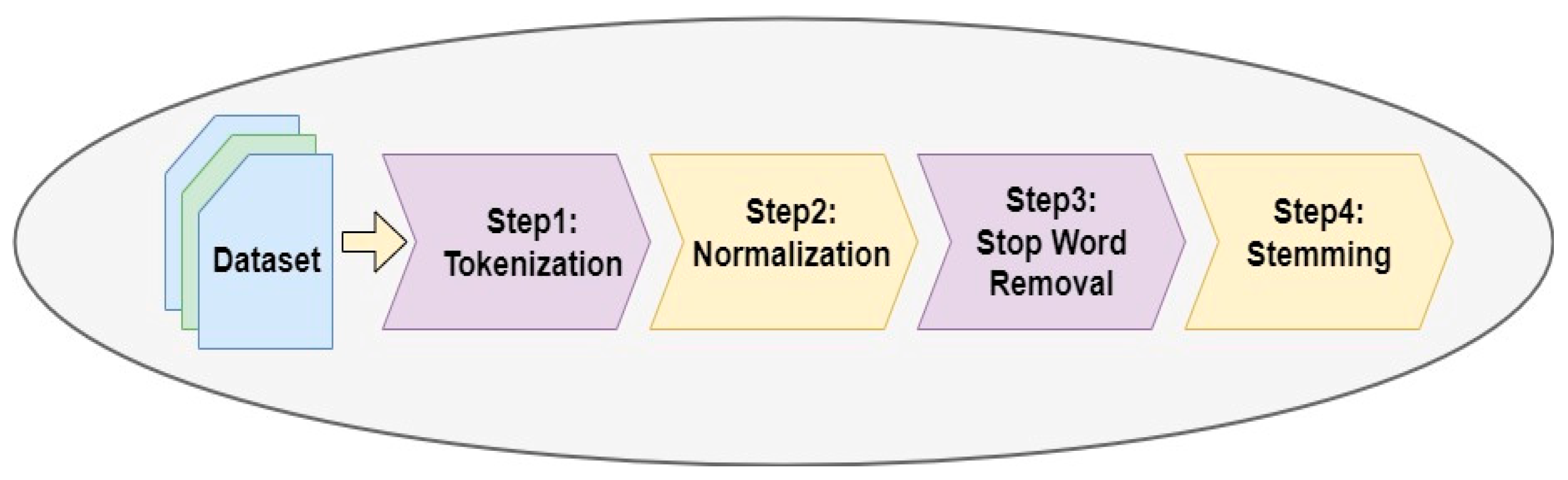
Pre-processing: It is the first step to take in STC. The data must be cleaned by removing unnecessary characters, words, symbols, and digits. Then, text representation methods can be applied. Pre-processing plays an essential role in building an efficient clustering system because short text data (original text) are unsuitable to be used directly for clustering.
(II)
Representation: Documents and texts are collections of unstructured data. These unstructured data need to be transformed into a structured feature space to use mathematical modelling during clustering. The standard techniques of text representation can be divided into the representation-based corpus and representation-based external knowledge methods.
(III)
Dimensionality reduction: Texts or documents, often after being represented by traditional techniques, become high-dimensional. Data-clustering procedures may be slowed down by extensive processing time and storage complexity. Dimensionality reduction is a standard method for dealing with this kind of issue. Many academics employ dimensionality reduction to lessen their application time and memory complexity rather than risk a performance drop. Dimensionality reduction may be more effective than developing inexpensive representation.
(IV)
Similarity measure: It is the fundamental entity in the clustering algorithm. It makes it easier to measure similar entities, group the entities and elements that are most similar and determine the shortest distance between related entities. In other words, distance and similarity have an inverse relationship, so they are used interchangeably. The vector representation of the data items is typically used to compute similarity/distance measures.
(V)
Clustering techniques: The crucial part of any text clustering system is selecting the best algorithm. We cannot choose the best model for a text clustering system without a deep conceptual understanding of each approach. The goal of clustering algorithms is to generate internally coherent clusters that are obviously distinct from one another.
(VI)
Evaluation: It is the final step of STC. Understanding how the model works is necessary before applying or creating text clustering techniques. Several models are available to evaluate STC.

3.1. Document Pre-Processing in Short Text Clustering

Document pre-processing plays an essential part in STC because the short text data (original text) are unsuitable to be used directly for clustering. The textual document likely contains every type of string, such as digits, symbols, words, and phrases. Noisy strings may negatively impact clustering performance, affecting information retrieval [51,52]. The pre-processing phase for STC enhances the overall processing [47]. In this context, the pre-processing step must be used on documents to cluster if one wants to use machine learning approaches [53]. Pre-processing consists of four steps: tokenization, normalization, stop word removal and stemming. The main pre-processing steps are shown in Figure 2.
According to [54], short texts have many unwanted words which may harm the representation rather than assist it. This fact validates the benefits of pre-processing the document in STC. Utilizing the documents with all their words, including unnecessary ones is a complicated task. Generally, words classified under particles, conjunctions and other grammar-based categories, which are commonly used, may be unsuitable for supporting studies on short text clustering. Furthermore, as suggested by Bruce et al. [55], even standard terms such as ‘go’, ‘gone’ and ‘going’ in the English language are created by the derivational and inflectional processes. They fare better if their inflectional and derivational morphemes are taken to remain in their original stems. This reduces the number of words in a document whilst preserving the semantic functions of these words. Therefore, a document free of unwanted words is an appropriate pre-processing goal [56,57].

3.1.1. Tokenization and Normalization

Tokenization is defined as a standard text representation that divides a flow of natural language text into distinct significant elements called tokens as part of the pre-processing [58]. Tokenization transforms the text from a document into data that can be analysed by machine learning methods. Generally, these algorithms segment the text into separate units by adding a space or some other kind of distinctive marker so that each team may be mapped to a different word in the text [55].
The normalization step aims to clean the data by removing unnecessary and noisy data, such as numbers, symbols, code tags and special characters. Whilst clustering search results, noise filtering is an essential task of the tokenizer. Likewise, the retrieved results, such as the contextual snippets supplied as input, include file names; URLs; characters that demarcate portions of whole documents, such as ellipsis characters (@, %, &, etc.) and other symbols whose meanings are not readily apparent. A reliable tokenizer needs to be able to recognize and get rid of this type of noise whilst it creates a token sequence. This step is necessary to carry out acceptable data representation and pre-processing.
As explained above, text tokenization and normalization transform the text into words or phrases by deleting extraneous strings of characters, such as punctuation marks, numerals and other strings of characters [59]. In essence, the white space is utilized to distinguish the collection of tokens that may be differentiated from one another. A text tokenization sample is illustrated in Figure 3. The text is displayed as a collection of tokens, with all of the characters written in lowercase, and white space is utilized to differentiate between each token. The commas, periods and other punctuation marks, along with any other special characters, are deleted.
The first step of the text pre-processing is describing the tokenization and normalization, which are as follows:
  • Remove numbers (2, 1…).
  • Remove punctuation marks (‘!’, ’, -, ”, :, ?, [], \, …).
  • Remove special characters (~, @, #, $, %, &, =, +).
  • Remove symbols (e.g., Applsci 13 00342 i001).
  • Remove non-English words, such as اسم.
  • Remove words with less than three letters.
Figure 4 shows the tokenization and normalization steps.

3.1.2. Stop-Word Removal

Stop words are utilized as a grammatical function of the language when a document lacks context instead of specifying a semantic function or meaning. Stop words are considered less useful in text than other terms. Generally, they have a direct effect on the meaning of the text. In most cases, documents include many unnecessary words in English. Stop words are typically utilized by writers to improve the structure of their writing linguistically. Examples of stop words include demonstratives such as ‘this’, ‘that’ and ‘those’ and articles such as ‘the’, ‘a’ and ‘an.’ Removing stop words from a document is typical and positively affects document clustering. This is because the capacity of the terms’ space is significantly reduced upon completion of word removal. Every language has its unique collection of stop words [56]. By removing these frequently used stop words from the text documents, the number of words each search term has to be matched against is reduced, significantly increasing the time it takes for queries to receive a result without affecting accuracy.
These words often communicate more grammatical functions than semantic functions, which may increase the conversational or informative aspects of the document’s content. Considering this, removing unnecessary words results in an improved ability to transmit the meaning of the text or document content and leads to an easier time understanding it using machine learning approaches. Many search engines have implemented stop word removal to help users or writers with queries obtain improved results by searching for information or meaning instead of searching for functional words [55]. Figure 5 displays the word document sample after removing stop words.

3.1.3. Stemming

This is the third step in pre-processing. We utilize stemmed words to represent the texts in this step. Stemming is a traditional shallow natural language processing (NLP) technique. Word stemming removes all prefixes and suffixes to obtain stem words [60]. Indexing and keyword filtering are crucial steps of stemming because they improve clustering faster and more accurately by reducing the vocabulary quantity and dependence on certain vocabulary forms [61]. Figure 6 illustrates how the stemming transforms the words ‘consultant’, ‘consultants’, ‘consulting’ and ‘consultative’ into a single stem, ‘consult’, which is also a word in the dictionary. However, this is not always the case; a stem may not always be an accurate word.

3.2. Document Representation

Even after the noise in the text has been removed during pre-processing, the text still does not fit together well enough to produce the best results when clustering. Therefore, focusing on the text representation step is essential, which involves converting the word or the full text from its initial form into another. Directly applying learning algorithms to text information without representing it is impossible [62] because text information has complex nature [63]. Textual document content must be converted into a concise representation before applying a machine learning approach to the text. Language-independent approaches are particularly successful because they are not dependent on the meaning of the language and perform well in the event of noisy text. As these methods do not depend on language, they are efficient [64].
Short text similarity has attracted more attention in recent years, and understanding semantics correctly between documents is challenging to understanding lexical diversity and ambiguity [65]. Representing short text is critical in NLP yet challenging owing to its sparsity; high dimensionality; complexity; large volume and much irrelevant, redundant and noisy information [1,66]. As a result, the traditional methods of computing semantic similarity are a significant roadblock because they are ineffective in various circumstances. Many existing traditional systems fail to deal with terms not covered by synonyms and cannot handle abbreviations, acronyms, brand names and other terms [67]. Examples of these traditional systems are BOW and TF-IDF, which represent text as real value vectors to help with semantic similarity computation. However, these strategies cannot account for the fact that words have diverse meanings and that different words may be used to represent the same concept. For example, consider two sentences: ‘Majid is taking insulin’ and ‘Majid has diabetes’. Although these two sentences have the same meaning, they do not use the same words. These methods capture the lexical features of the text and are simple to implement; however, they ignore the semantic and syntactic features of the text. To address this issue, several studies have expanded and enriched the context of data from an ontology [68,69] or Wikipedia [70,71]. However, these techniques require a great deal of understanding of NLP. They still use high-dimensional representation for short text, which may lead to wasting memory and computing time. Generally, these methods use external knowledge to improve contextual information for short texts. Many short text similarity measurement approaches exist, such as representation-based measurement [72,73], which learn new representations for short text and then measure similarity based on this model [74]. A large number of similarity metrics have previously been proposed in the literature. We choose corpus-based and knowledge-based metrics because of their observed performance in NLP applications. This study explains several representation-based measurement methods, as shown in Figure 7.

3.2.1. Non-DL Measures

In this section, the literature is comprehensively reviewed to understand the research attempts and trends in measuring the similarity of STC, including corpus-based measures and knowledge-based measures.

Bag of Words Model

According to [75,76], BOW is the most traditional text representation method used to simplify the data to be more suitable in the processing stage by considering the text data as groups of words. It is widely used in IR and NLP because of its simplicity and efficiency, where it uses simple words or phrases as features to represent text. The difficulties with text processing stem from the fact that text data’s syntactic and semantic content is challenging to quantify. Creating a comprehensive model of all text data is challenging. Thus, the current text analysis approach usually represents a text document by reducing the text structure complexity and simplifying text documents. BOW is a text document representation that treats a written document as a BOW, ignoring word order and grammar. Figure 8 illustrates how BOW can be used to represent two texts. Stop words are removed, such as ‘a’ and ‘is’, from practical processing to underline the relevance of other words. In Figure 8, we see a fixed-length vector is represented for each short text. The value assigned to each dimension in the vector represents the term frequency (tf) in the corresponding section of the text document. BOW can help text representation by simplifying the text document, but it may not distinguish the difference between two documents with the same bag of words but in different sequences.
However, the BOW model has several drawbacks. Some corpora, such as social media corpora, include slang and misspelt words, which result in a high-dimensional feature space. Furthermore, these models cannot process complex word meaning differences, such as synonyms and polysemy. BOW has a weak sense of the semantics of the words, or more formally, the distances between words [77].

Vector Space Model (VSM)

It is a traditional method for measuring the distance between text documents after simplifying text data by BOW, where term weight vectors represent the original texts [27,78]. VSM uses document-level word occurrences as its representational basis. Using different term-weighting methods, a document with basic terms can be mapped into the high-dimensional term feature space. The term-weighting algorithms are utilized to determine which terms are most significant. The performance of text analysis can be improved by using the appropriate term weighting. Term weighting aims to assess the significance of terms within a given document or corpus. Several different term-weighting methods are available. Short text has a limited length of the text, and the size vocabulary of words in the corpus is often quite large. Therefore, when calculating similarity/distance using cosine similarity or Euclidean distances [29], the VSM-based representation for short texts produces sparse and high-dimensional vectors, which are less discriminative.
Topic-model-related methods are utilized to learn high-level semantic text representations to alleviate the disadvantages of VSM with a short text [1]. Based on the frequencies of the terms in the original text documents, the weights of the terms are calculated. The VSM transforms the term frequency into a numerical vector. Although simple to set up, VSM has drawbacks, including high dimensionality and sparsity. These weaknesses of VSM become even more apparent when dealing with short text data. In addition, the global term weighting is calculated by querying all documents. Generally, the common word weighting strategies can be divided into local and global term weighting schemes [27,79].
 I. 
Local term weight
It is the term frequency value within the document derived by several methods [78]. For example, the most important and commonly used local weighting schemes, as shown in Table 1, are term presence (tp), term frequency (tf), augmented term frequency (atf), the logarithm of term frequency (ltf), and BM25 term frequency (btf). The most notable and common representation is tf, which indicates the number of occurrences of the term in the document. Thus, it emphasizes the words that appear more frequently. tp is the simple binary representation, which ignores the number of appearances of the term in the document. This can be useful when the number of times a word appears is unimportant. tp and tf are combined in the atf scheme. It tries to instil confidence in any term in the document and add confidence to frequently occurring terms. ltf is used as a logarithmic function to set within-document frequency because a term that appears five times in a document is not always five times as important as a term that occurs once in that document.
 II. 
Global term weight
It calculates the weight by collecting all training documents [78]. It tries to grant a discrimination value to each term and emphasize discriminatory terms. For example, the most popular and notable metric global term weighting schemes shown in Table 1, such as idf, bidf, and pidf, are unsupervised because they do not use the category label information from training documents. In idf, the main idea of the inverse document frequency is to provide high weights for rare terms and low values for standard terms. This scheme is calculated using the logarithmic ratio of the number of documents in a collection to the number of documents containing a specific term. The versions of bidf and pidf are the other two approaches to idf. The premise behind idf, bidf and pidf is that a phrase that appears less frequently in documents is more discriminatory. This strategy works well in IR, but it is inappropriate for text categorization and text clustering because these tasks are designed to distinguish between categories, not documents [78].
Table 1 shows that a and b represent the number of training documents in group one, including the terms t i and c; d represents the number of training documents in group two, including term t i . N represents the number of documents in the corpus, N = a + b + c + d.
Finally, text data are represented by considering the context or topic of text documents or segments. However, a document is characterized by its topic or the keywords that stand out the most. Consequently, several topics can be associated with a single document, and documents are clustered according to the number of topics they share.

Latent Dirichlet Allocation (LDA)

LDA is defined as generative probabilistic modelling for text data. LDA is one of the most widely used methods in topic modelling, and it was developed in 2003 by [73]. The fundamental concept is based on the texts represented as random mixtures from latent topics, where the distribution of the words characterizes a topic. The simplicity and effectiveness of LDA lead to its widespread use. LDA uses word probabilities to represent topics. The words with the highest probabilities in each topic usually give a good idea of what the topic is using word probabilities from LDA.
LDA assumes that each text may represent a probability distribution across latent topics, with a shared Dirichlet prior across all texts. Each latent topic is represented as a probabilistic distribution from words in the LDA model, and the word distributions of topics share a common Dirichlet prior. Assuming a corpus D consisting of M documents, with document d having N d words ( d ∈ 1, …, M ), LDA models D using to the following generative process [73]:
(a)
Select a multinomial distribution φ t for topic t ( t ∈ [1, …, T]) from a Dirichlet distribution with parameter β .
(b)
Select a multinomial distribution θ d for document d ( d ∈ [1, …, M]) from a Dirichlet distribution with parameter α .
(c)
For a word w n ( n ∈ [1, …, N d ]) in document d ,
  • Choose a topic z n from θ d .
  • Choose a word w n from φ z n .
In the generative process described above, words in texts are the only observable variables, whereas others ( φ and θ ) are latent variables. ( α and β ) are hyperparameters. The probability of observed data D , as shown in Figure 9, is calculated and acquired from the data corpus by using the following equation [80]:
p D | α , β = d = 1 M p θ d α n = 1 N d z d n p z d n θ d p ( w d n | z d n , β ) d θ d
Several methods for estimating LDA parameters have been proposed for parameter estimation, inference and training for LDA, such as Gibbs sampling [81].
 I. 
Gibbs sampling
It is a powerful and simple technique in statistical inference. It is a Monte-Carlo–Markov-chain algorithm. Gibbs sampling produces a sample from a joint distribution when only conditional distributions of each variable can be efficiently computed. Many researchers have used this technique for the LDA [82,83,84].

Dirichlet Multinomial Mixture (DMM)

The other technique is based on model-level improvements, in which standard procedures impose additional constraints on model assumptions to generate topics. Assuming that in traditional models, each document is composed of several topics, given that each short text document has only a few words. The DMM [66] model assumes that there is only one topic covered in each document. The constraints on these models are excessive. The number of relevant topics depends on the information in the various texts. As a result, simply putting such restrictions has the potential to cause noise, so this technique may be less effective and less generic. A corpus is a collection of search results composed of D . The character D denotes the number of documents in the corpus. Each   d includes a group of words w   ϵ   1 , 2 , , N d . Figure 10 describes the DMM model D. The DMM models work according to the following process:
(a)
Sample θ = 1 , 2 , , n from a Dirichlet distribution with parameter α = λ 1 , λ 2 , , λ n .
(b)
For each topic t = 1 , 2 , , n T , the sample Ø from a Dirichlet ( β ) , where β = λ β 1 , λ β 2 , , λ β n .
(c)
For a   d   d   ϵ   1 , ,   N : in = d .
  • A topic z n 1 , 2 , , T c c is selected from multinomial α , where α = 1 , 2 , , n represents the topic distribution in the corpus.
  • The word count N d is selected, and a word w d from d from multinomial β is also independently selected, where β = β 1 , β 2 , , β n represents the word topic distribution in the corpus.
A DMM-based method for STC was suggested by [66]. However, how to create an effective model remains unclear. Based on BOW, most of these methods are trained, which are shallow structures that cannot maintain semantic similarities [25]. In Equation (2), the probability of observed data D is calculated and maximized to infer the latent variables and hyperparameters [66]:
p d | α , β = l = 1 T α l N d ! w = 1 V N d w ! w = 1 V β w t N d w ,
where α denotes the topic Dirichlet prior parameters and the distribution of words over topics from the Dirichlet distribution; for a specific β , the vocabulary size is represented by the letter V . The frequency of the word W in d is N d w . Additionally, the number of words is N d . For corpus-level topic distributions, the Dirichlet-multinomial pair is (   α , θ   ). A DMM output matrix has rows for documents and columns for topics. The labelled one is assigned to the cell with the coordinates (i,j) if the document d i belongs to the topic t j .

Latent Semantic Analysis (LSA)

This model is a technique in text representation that can be used for modelling the conceptual relationship among several documents based on their set of words, which can be computed as semantic information using this model. One of the methods for improving the text representation model is using semantic information [85]. This concept is founded on the premise that words with lexical distinctions frequently appear in similar documents and have similar meanings. LSA is a promising method for constructing a latent semantic structure in textual data and identifying relevant documents that do not share common words. It also reduces the sizeable term matrix to a smaller one and provides a stable clustering space. LSA differs from standard NLP because it does not use dictionaries, knowledge bases, grammar or syntactic parsers. It accepts as input only raw text that has been split into meaningful paragraphs. In a matrix, LSA represents the text that is described. Each column of the matrix refers to a passage where the word appears, and each word corresponds to one row in the table. The matrix cells show how often the term appears in the paragraph, as shown in Figure 11.

Word Embedding

It is a neural network representation learning approach that be capture syntactic and semantic similarities between words [86]. Word embedding aims to map the words in unlabelled text data to a continuously valued low-dimensional space to capture the similarities between words [87]. It creates latent feature vectors for words to maintain their syntactic and semantic information. The efficiency of word representations relies on implicit relations between words in the corpus. The three common approaches for word embedding learning are Word2Vec [86], Doc2Vec and Glove [88]. Owing to vocabulary mismatches, the noisy nature of microblogging data, and a lower number of word co-occurrence in text data, applying these pre-trained word embedding algorithms to short text input is limited [89]. Most word embedding strategies can only learn one vector for each word [90]. Many words, however, have multiple meanings. For example, the word apple can have numerous semantics. When used in the statement ‘I like eating apples’, it refers to a type of food. It refers to the name of a technological corporation when it appears in the sentence ‘We went to the Apple store yesterday’.
 I. 
Word2Vec
It was proposed by [86] as a collection of related models used to generate word embedding. It utilizes a ‘shallow’ neural network capable of quickly processing billions of word occurrences and producing syntactically and semantically relevant word representation models. The authors also investigated two models of word-embedding learning: skip-gram and continuous bag of words (CBOW). The former takes in a word and predicts the context words, whereas the latter indicates the target word using a source of context words [20].
 II. 
Doc2Vec
It was proposed by [77] as a straightforward extension to Word2Vec [86] for extending learning embeddings from words to word sequences. Doc2Vec is agnostic to the granularity of the word sequence, which can be a word n-gram, sentence, paragraph, or document. Doc2Vec also produces sub-par performance compared with vector-averaging methods based on previous studies [46].
 III. 
GloVe (Global Vectors for Word Representation)
It is a log-bilinear regression model proposed by [88]. It attempts to resolve the disadvantages of global factorization approaches (e.g., latent semantic analysis [91]) and local context window approaches (e.g., skip-gram model [73]) on the word analogies and semantic relatedness task. GloVe’s global vectors are trained via unsupervised learning on a corpus of aggregated global (word x word) co-occurrence information. GloVe’s goal is to factorize the log-count matrix and find a word embedding that meets this criterion [92]. Owing to vocabulary mismatch, a lower number of word co-occurrence in short text data and noisy nature of microblogging data, the applicability of these pre-trained word-embedding models to short text data is minimal [89].

Pseudo

One typical strategy to compensate for the sparsity of short texts is to use ‘pseudo-relevance feedback’, which involves enriching the original short text corpus with supplementary data from semantically related long texts. This can be accomplished by submitting the short text data as input to a search engine as queries, which returns a set of the most relevant results [48].
Although the pseudo-relevance feedback-based data augmentation strategy appears promising, this strategy’s drawbacks should be noted. Such a process is inherently noisy, and some of the auxiliary material may be semantically unrelated to the original short texts. Similarly, unconnected or loud extra issues may have a negative impact. As a result, combining short texts with long texts or themes that are semantically unrelated to the short texts may degrade the performance of the short texts. The problem can become even more severe because there is no labelling information to guide the selection of auxiliary data and auxiliary topics for unsupervised learning of short texts.
Another strategy is to combine short texts into large pseudo-documents and then use standard topic models to infer topics from these pseudo-documents [49,93]. This strategy is highly data dependent, so extending it to deal with more generic forms, such as questions/answers and news headlines, is complex. One of the current strategies’ main weaknesses is that the exact short text may contain different topics and therefore can be related to more than one topic. The assumption that only one topic is addressed in each text is inappropriate for these short texts. Furthermore, most standard similarity measures depend heavily on the co-occurrence of words in two documents. As they have no words in common, aggregating a large number of short texts into a small number of pseudo-documents is challenging [94].

External Knowledge

One of these strategies is to use external knowledge as a source of enrichment. [95] suggested a strategy that can be summarized by using external knowledge to uncover hidden topics to address the data sparsity issue. The dual-LDA model was proposed by [48], which generates topics using short texts and related lengthy texts. Document expansion strategies usually expand feature vectors by adding relevant terms [48,70,96]. External knowledge sources such as Wikipedia [70], WordNet [96] and ontologies [48] are commonly used for document expansion. However, owing to semantic incoherence, short text from social media enriched with these static external sources provides insufficient information [45]. Given the dynamic nature of short text data on the web, comprehensive background information from an external knowledge sources such as Wikipedia may not accurately capture the meaning of context-sensitive short texts. In addition, external knowledge such as Wikipedia may not always be available on the web or may be too costly.
 I. 
WordNet
It is defined as a vast lexical database. Nouns, verbs, adverbs and adjectives are grouped into sets of cognitive synonyms. Each of these expresses a distinct concept. Conceptual-semantic and linguistic relationships link synsets together [96]. WordNet is helpful for computational linguistics and NLP because of its structure.
WordNet resembles a thesaurus because it groups words depending on their meanings. Nevertheless, some key distinctions are noted. Firstly, WordNet connects not just word forms—letter strings—but also precise meanings of words. Therefore, words in the network close to one another are semantically disambiguated. Secondly, WordNet labels the semantic relationships between words, whereas thesaurus groupings follow no defined pattern other than meaning similarity. One issue with using WordNet is that it does not cover the most recent topics.
 II. 
Wikipedia
It is a free online encyclopaedia where experts and volunteers express various concepts. It contains a substantial knowledge base: history, art, society and science. It is an ideal knowledge base for readers and scholars seeking information and modern data-mining algorithms looking for supplementary data to increase performance. Each Wikipedia entity’s article contains a comprehensive explanation from multiple perspectives. Furthermore, the content of these articles is organized logically [70]. This benefit may make retrieving entity information easier for autonomous learning systems.
Many links in an entity corpus can indicate a semantic relationship between connected entities, aiding automatic concept recognizers in finding related data. Wikipedia is used to improve the short text quality, where clustered short text is enhanced based on the enriched representation. They enrich the short text with information from the Wikipedia database. The concepts from Wikipedia are used to improve short text clustering. Related concepts are extracted and computed using a combination of statistical laws and categories. Then, the semantically related concept sets are built to extend the eigenvector of a short text to supply its semantic features.
However, non-deep-learning measures have several disadvantages. Table 2 illustrates and summarizes the advantages and disadvantages of non-deep-learning measures.

3.2.2. Deep Learning Measures

Deep learning is currently the undisputed best technology for supervised machine learning, particularly for numerical data classification and clustering. However, its use in unsupervised learning has been more limited and recent [97]. Recently, deep learning has been used for unsupervised tasks, including topic modelling and clustering [98]. In many cases, the training goals are still the same, and deep learning appears to be most helpful with feature extractors such as convolutional neural network (CNN) [99]. The process of transforming input data into a collection of features is known as feature extraction [99]. Feature extraction is a technique used in machine learning to improve the efficacy of learning algorithms by transforming training data and augmenting them with extra features to make machine learning algorithms much more adequate.
Deep learning is one of several strategies utilized for short text. Recently, short text has grown on social media platforms, where people can share information and assemble societal opinions through short text conversation. The short text data comprise sparse word co-occurrences; it is challenging for unsupervised text mining to uncover categories, concepts or subjects within the data [89]. During the last few years, deep learning methods have shown much power to extract features autonomously and automatically from raw data [100]. In general, a deep learning model is constructed of many layers of neural networks. Each layer comprises numerous basic signal-processing units known as neurons. The basic structure of neurons is depicted in Figure 12.
A neuron can take an input signal and produce an output signal using the neuron’s strategies it has learned. Raw information is gradually processed as it passes through multiple interconnected layers of neurons. The structure of a multi-neuron neural network is illustrated in Figure 13. The artificial neuron network uses a massive scale of basic units to handle input in a similar way that the human brain does. Recently, deep text representation has been learned using supervised deep learning techniques [25], depending on shallow-to-deep auto-encoders utilizing recurrent neural networks (RNNs) [101], CNNs [101], long short term memory (LSTM), bidirectional long short term memory (Bi-LSTM) and recursive tree LSTM [102]. Nevertheless, in many applications, a dense representation should be discovered in an unsupervised fashion to identify clusters, concepts or topics in the short text. Two elementary procedures, convolution and pooling, form the basis of deep neural network models. In text data, the convolution procedure is the product of a sentence vector and a weight matrix, with each element contributing to the whole. When attempting to extract features, convolution operations are performed. Features with a negative impact can be ignored, and only feature values with a significant effect on the work at hand are taken into account, thanks to pooling operations. The most common pooling operation is called ‘max pooling’. It involves picking the highest value in a particular filter space [103]. In this section, the literature is extensively reviewed to measure the similarity of short text based on deep learning measures. The most common models are listed below.

Convolutional Neural Networks

It is a popular deep learning approach; specific techniques use CNNs as feature extractors. Recently, the CNN has improved performance in many NLP applications, including relation classification [104], phrase modelling [105] and other traditional NLP tasks [106,107]. This is because the CNN is the most popular nonbiased model and applies convolutional filters to capture local features. A reliable feature function that extracts higher-level characteristics from constituent words or n-grams became necessary with the widespread use of word embeddings due to its capacity to represent words in a dispersed space. The self-taught CNN ( STC 2 ) was proposed by Xu et al. [25] to learn implicit features from short texts for short text representation. Short text representation learning has also been implemented using neural-network-based techniques. The proposed model needs two different raw representations of short text: binary coding representations of short text-based dimensionality reduction on term-frequency vectors and word embedding representations of short texts pre-trained from large external corpora. The input for CNNs is word-embedding representations of short texts, and the binary codes are utilized as data labels to train the CNN model. After the CNN is trained successfully, the deep representations for short text are taken from the last hidden layer of the CNN. However, short texts are usually sparse, so the deep features learned by neural network-based techniques may not accurately represent the short text.

Recurrent Neural Networks

Recently, neural networks such as recursive neural networks (RecNN) [108] and RNN [109] have demonstrated superior performance in creating text representations via word embedding. RecNN has high temporal complexity in building the textual tree, whereas RNN, which uses the hidden layer computed at the last word to represent the text, is a biased model in which later words are more prominent than early words [110]. By contrast, non-biased models may extract the learnt representation of a single text from all of the words in the text using non-dominant learning weights [25]. In recent years, RNNs have seen widespread adoption in research focusing on sequential data types, such as text, audio and video. However, when the input gap is wide, the RNN cannot learn important information from the input data. The problem of long-term dependencies is well-handled by the LSTM after gate functions are introduced into the cell structure [111].

Long Short-Term Memory

The LSTM networks are a subclass of RNNs. RNNs can remember the previous words, capturing the context, which is crucial for processing text input. RNNs have the issue of long-term reliance because not all the past content is relevant to the following word/phrase. To counteract this issue, LSTMs are developed. Owing to the gates in LSTMs, the network can pick and choose which bits of information to remember [111]. The LSTM framework is widely used for determining how similar two sections of text are semantically [112]. To predict the similarity of sentences, Tien et al. [113] utilized a network that combines LSTM and a CNN to create sentence embedding using pre-trained word embeddings. Tai et al. [114] suggested an LSTM design to measure the semantic similarity between two supplied sentences. Tree-LSTM is then trained over the parse tree to provide sentence representations. A neural network is trained with these phrase representations and determines the absolute distance and angle between the vectors.

Bidirectional Long Short-Term Memory

Bidirectional RNNs are just two independent RNNs combined. This structure enables the networks to contain both backward and forward sequence information at each time step. Bi-LSTMs use two LSTMs that run in parallel in order to fully capture the context [102]. By running the inputs in two directions, one from the past into the future and the other from the future into the past, one may preserve information from both the past and the future simultaneously, making this method superior to the more common unidirectional one. Like NLP, there are occasions when knowing what comes next is just as important as knowing what came before. To estimate the model’s semantic similarity, He and Lin [115] presented a hybrid architecture based on Bi-LSTM and CNN to fully capture the context. The approach takes advantage of Bi-LSTM to perform context modelling. Two LSTMs’ hidden states are used to generate vectors that are then compared using a comparison unit, resulting in a model of paired word interactions.
Mueller and Thyagarajan presented a MaLSTM [72], which is a Siamese deep neural network that uses LSTM networks with connected weights as sub-modules to learn presentations for sentences. MaLSTM receives sentence pairs, initially expressed as word embedding vectors, as inputs. MaLSTM is trained to utilize a loss function based on the Manhattan distance to learn new representations for sentences.

Bidirectional Encoder Representations in Transformers (BERT)

It is a computational method that allows machine learning models to be trained on textual data. BERT learns contextual embeddings for words as a result of the training procedure [116]. Following the computationally expensive pretraining, BERT can be fine-tuned with lower resources on smaller datasets to optimize its performance on specific tasks. It refers to bidirectional encoder representations in transformers. In contrast with modern theories of language representation [117], pretraining deep bidirectional representations from the unlabelled text is the goal of BERT, and it does so by concurrently conditioning the left and right context across all layers [118]. For this reason, the pre-trained BERT model may be fine-tuned with a single extra output layer to provide state-of-the-art models for various tasks, including Q&A and language inference, without significant task-specific architecture alterations.
Many different types of NLP tasks have been improved using language model pre-training [119]. Paraphrasing [120] and natural language inference [121] are examples of sentence-level tasks that aim to predict relationships between sentences by analysing them holistically. Named entity recognition and Q&A are examples of token-level tasks that require models to produce fine-grained output at the token level [122], as shown in Figure 14.
In Table 3, the deep learning similarity measure works of literature are illustrated and summarized.

3.3. Dimensionality Reduction

It is commonly used in machine learning and big data analytics because it aids in analysing large, high-dimensional datasets. It can benefit tasks like data clustering and classification [126]. Recently, dimensional-reduction methods have emerged as a promising avenue for improving clustering accuracy [127]. Text sequences in term-based vector models have many features. As a result, memory and time complexity consumption are prohibitively expensive for these methods. To address this issue, many researchers use dimensionality reduction to reduce the feature-space size [101]. Existing dimensionality reduction algorithms are discussed in depth in this section.

3.3.1. Principal Component Analysis (PCA)

It is the most common technique in data analysis and dimensionality reduction, and almost all scientific disciplines use it. PCA seeks to find the most meaningful basis for re-expressing a given dataset [101]. This entails identifying new uncorrelated variables and maximizing variance to maintain as much variation as possible [128]. This new basis is expected to reveal hidden structures in the dataset and filter out noise [129]. PCA has numerous applications, including dimensionality reduction, feature extraction, data compression and visualization.
A dataset with observations on p numerical variables for each of n entities or individuals is the standard context for PCA as an exploratory data analysis tool. These data values define p n-dimensional vectors x 1 , ,   x p , or equivalently, an x × p data matrix X , with the j th column containing the vector x j of observations of the j th variable. We are looking for a linear combination of the columns of matrix X with the slightest variance. The linear combination can be written as the following equation (see Equation (3)) [128]:
j = 1 P a j x j = X a ,  
where a represents a vector of constants a 1 ,   a 2 , , a p . This linear combination’s variance is given as Equation (4):
V a r x a = a T s a   ,
where S represents the sample covariance matrix. The goal is to find the linear combination with the least amount of variance. This is equivalent to maximizing Equation (5):
a T s a λ a T a 1   ,
where λ is a Lagrange multiplier.
ICA is a statistical modelling method that expresses observed data as a linear transformation [130]. A statistical ‘latent variables’ model can be used to rigorously define ICA [131]. Assume we find n linear mixtures x 1 , , x n of n independent components. The x j for all j can be computed as in Equation (6):
x j = a j 1 s 1 + a j 2 s 2 + + a j n s n
Sometimes we require the columns of matrix A ; denoting them by a j , the model can also be written as Equation (7):
X = i = 1 n a j s i

3.3.2. Linear Discriminant Analysis (LDA’)

It is a standard data-mining algorithm used for supervised or unsupervised learning. LDA is commonly used for dimensionality reduction [132]. It determines the projection hyperplane with the lowest interclass variance and the most significant distance between the projected means of the classes [133]. LDA is beneficial when the within-class frequencies are unequal and their performances have been assessed using randomly generated test data.
Let us say X j d × n j , which are d-dimensional samples, and y i 1 , 2 , , k denotes the class label of the i th sample, where n is the number of documents, d is the data dimensionality and k is the number of classes. Equations (8)–(10) calculate the number of samples in each class:
n = j = 1 k n j
n j = x w i x μ i x μ i T
μ i = 1 N i x w i x
In discriminant analysis [134], three scatter matrices are defined as within-class, between-class and total scatter matrices, as shown in Equations (11)–(13):
S w = 1 n j = 1 k x X j x c ( j ) x c ( j ) T
S b = 1 n j = 1 k n j c ( j ) c c ( j ) c T
S t = 1 n i = 1 n x i c x i c T
where c j It is the centroid of the j th class and c is the global centroid. It follows from the definition that S t = S b + S w . Furthermore, trace ( S w ) measures the within-class cohesion, and tracing ( S b ) measures the between-class separation.

3.3.3. T-Distributed Stochastic Neighbour Embedding (t-SNE)

T-SNE is a method for reducing dimensionality. Dimensionality reduction is significant in extracting the essential features from a complex set of expression profiles from various samples. This method is commonly used for low-dimensional feature space visualization [135]. This entails mapping the high-dimensional state-vectors onto a low-dimensional space (typically a plane) while maintaining critical information about the relatedness of the component samples. SNE converts high-dimensional Euclidean distances into conditional probabilities representing similarities [136]. The conditional probability p j 1 is computed as follows:
p j 1 = exp x i x j 2 / 2 σ i 2 k 1 exp x 1 x k 2 / 2 σ 1 2 ,
where σ i is the variance of the Gaussian that is centred on datapoint x i . To calculate the similarity of point y j with y i , the following is calculated:
q j 1 = exp y i y j 2 k 1 exp y 1 y k 2
SNE uses a gradient descent method to minimize the sum of Kullback–Leibler divergences over all data points. Cost function C is denoted by Equation (16):
C = i K L P i Q i = i j p j i log p j i q j i
SNE performs a binary search for the value of Q i to produce a P i with the user-specified fixed perplexity. The perplexity is defined as Equation (17):
p e r p p i = 2 H p i   ,
where H p i It is the Shannon entropy of Pi measured in bits, as shown in Equation (18):
H P i = j p j i log 2 p j i
The minimization of the cost function is performed using a gradient descent method, as illustrated in Equation (19):
δ C δ y i = 2 j p j i q j i + p i j q i j y i y j
The spring force between y i and y j is proportional to its length and stiffness, which is the mismatch p j i q j i + p i j q i j between the pairwise similarities of the data points and the map points.
In addition, to determine the changes in the coordinates of the map points at each iteration of the gradient search, the current gradient is added to an exponentially decaying sum of previous gradients. The gradient update with a momentum term is given mathematically by the following Equation (20):
Y t = Y t 1 + η δ C δ Y + α t Y t 1 Y t 2 ,  
where Y t represents the solution at iteration t , η represents the learning rate and α t represents momentum at iteration t .

3.3.4. Uniform Manifold Approximation and Projection (UMAP)

It is an embedding method for dimensionality reduction and a newly proposed multivariate learning method for adequately representing the local structure while better incorporating the global structure [137]. UMAP scales well with massive datasets. UMAP uses a high-dimensional graph representing the data points to generate the fuzzy topological structure. The created high-dimensional graph is a weighted graph, with edge weights indicating the probability that two points are related. UMAP computes the similarity between high-dimensional data points using an exponential probability distribution, as given in Equation (21) [126]:
p i j = e x p d x i , x j ρ i σ i   ,
where d x i , x j represents the distance between the i th and j th data points, and ρ i is the distance between the i th data point and its first nearest neighbor(s). When the weight of the graph between i and j nodes is greater than the weight between j and i nodes, UMAP employs a high-dimensional probability symmarization, as shown in Equation (22):
p i j = p i j + p j i p i j p j i
UMPA in the graph must indicate k, the number of nearest neighbours, where k is calculated by Equation (23):
k = 2 i p i j
UMAP uses a probability measure for modelling distance in few dimensions, as shown in Equation (24):
q i j = 1 + a y i y j 2 b 1
For default UMAP, a ≈ 1.93 and b ≈ 0.79. UMAP employs binary cross-entropy (CE) as a cost function due to its ability to capture the global data structure, as illustrated in Equation (25):
C E ( P , Q ) = i j p i j log p i j q i j + 1 p i j log 1 p i j 1 q i j ,
where P represents the probability similarity of high-dimensional data points and Q represents low-dimensional data points.

3.4. Similarity and Distance Measure

The similarity measure determines the similarity between diverse terms, such as words, sentences, documents or concepts. The goal of determining similarity measures between two terms is to determine the degree of relevance by matching the conceptually similar terms but not necessarily lexicographically similar terms [138].
Generally, the similarity measure is a significant and essential component of any clustering technique. This is because it makes it easier to measure two things, group the most similar elements and entities together and determine the shortest distance between them [139,140]. In other words, distance and similarity have an inverse relationship, so they are used interchangeably. In general, similarity/distance measures are computed using the vector representations of data items.
Document similarity is vital in text processing [141]. It calculates the degree to which two text objects may be identical. Nonetheless, the similarity and distance measures are used as a retrieval module in information retrieval. Similarity measurements include cosine, Jaccard and inner products; distance measures include Euclidean distance and KL divergence [142]. An analysis of the literature studies shows that several similarity metrics have been developed. However, none of the similarity metrics appears to be the most effective for any research [143].

3.4.1. Cosine Similarity

It is one of the primary measures utilized to compute the similarity between two terms. The cosine similarity is used with documents in several applications, including text mining, IR and text clustering [144]. We choose the documents t a and t b , to define the similarity between the two documents using the cosine similarity method. We used Equation (26) for cosine similarity, as shown below:
C o s i n e   s i m i l a r i t y   b t a , t b t a . t b t a × t b .  
where t a and t b are interpreted as m-dimensional vector models by using the term set T { t 1 t m }. They represent all terms with weights together in the document by a specific dimension that is also non-negative. Therefore, the cosine similarity scale runs between 0 and 1.
Cosine similarity is one of the main qualities and essential characteristics, independent of the document length, which makes it distinct and characterized by cosine similarity. For instance, if we have two copies of the same document and want to determine the cosine similarity between them, we will combine document d to create the new pseudo document d 0 . Consequently, the cosine similarity between documents d and d 0 is equal to 1. According to the evidence presented here, these two documents are the same.

3.4.2. Jaccard Coefficient

The Tanimoto coefficient or Jaccard coefficient is a common statistical coefficient found in NLP [144]. The Jaccard coefficient is a measurement unit that determines how similar two items are by dividing the intersection of the objects by their union. The Jaccard coefficient is applied to the text document to compare the sum of the weight of terms found in either of the two documents and the total weight of shared words, but they must not be shared terms. Equation (27) is a presentation of the mathematically correct definition of the Jaccard coefficient:
Jaccard   t a ,   t b = t a .   t b t a 2 + t b 2 t a .   t b
The Jaccard coefficient is a measure of similarity with a range of [0, 1]; when t a and t b are mutually exclusive, the coefficient is 0, and when they are equivalent, it is 1.

3.4.3. Euclidean Distance

Euclidean distance, also known as the Euclidean metric, is a frequently used distance measure in clustering algorithms, including clustering text and is the default measure of distance in the K-means algorithm [144]. For instance, to calculate the distance between two documents, d a and d b are represented by their term vectors t a and t b successively; the term set is T = t 1 t m . Equation (28) calculates the Euclidean distance between two documents:
Euclidean   t a , t b = t = 1 m w t , a w t , b 2

3.5. Clustering Algorithms

Clustering methods divide a collection of documents into groups or subsets. Cluster algorithms seek to generate internally coherent clusters yet distinct from one another. In other words, documents inside one cluster must be similar as feasible, whereas documents in different clusters should be as diverse as possible. The clustering method splits many text messages into many significant clusters. Clustering has become a standard strategy in information retrieval and text mining [145]. Concurrently, text clustering faces various challenges. On the one hand, a text vector is a high-dimensional vector, typically ranging in the thousands or even the ten thousand dimensions. On the other hand, the text vector generally is sparse, making it challenging to identify the cluster centre. Clustering has become an essential means of unsupervised machine learning, attracting many researchers [146,147].
In general, there are three types of clustering algorithms: hierarchical-based clustering, partition-based clustering and density-based clustering. We quickly discuss a few traditional techniques for each category; clustering algorithms have been extensively studied in the literature [148,149].

3.5.1. Hierarchical Algorithms

Hierarchical algorithms create a hierarchy of clusters. Hierarchical clustering algorithms have become the standard method for document clustering [150] by combining the ideal measure similarities such as cosine similarity, Jaccard similarity coefficient and Dice coefficient.
The most popular text clustering technique that produces nested groups in the form of a hierarchy is called hierarchical clustering. To use this strategy, the category must be hierarchical. Generally, the relevant objects will be updated if the category changes. The output of using a hierarchical clustering method is a single-category tree. A sample of hierarchical clustering is shown in Figure 15; each class node has several child nodes, and a brother node is a division of its parent nodes.
This can form extended, almost identical clusters. For clusters of comparable sizes, the complete-link approach is preferable (in volume). The similarity between two groups can be defined as the degree to which their two most similar objects and most distinct [150,151].
As a result, this method allows for data classification at various granularities. In general, hierarchical clustering is accurate. However, each class must integrate and compare the overall similarity of all classes to choose the two more similar classes, which is comparably slow. Another problem of hierarchical clustering is that once a stage merge or split is finished, it cannot be halted, making it impossible to correct a mistake [147]. The hierarchical clustering techniques may be classified into two groups based on the formation of the category tree methods: the top-down split technique and the bottom-up integration technique [151].
Bottom-up (merge-up) hierarchical clustering starts with a single item. It begins with an item as a solitary category and then consistently combines two or more appropriate categories. The hierarchical clustering does not loop as long as the stop criteria are fulfilled (the number of parameters is generally K, where K = Number of clusters). The bottom-up hierarchical clustering method is viewed as constructing the tree, consisting of data on the class hierarchy and the degree of similarity between all classes. Hierarchical clustering has the following advantages: it may be used with any shape, degree of similarity or distance and it features an inherently adaptable clustering granularity. One drawback of hierarchical clustering is the ambiguous termination condition: once the clustering is complete, it should define the human experience. Often, this technique cannot be rebuilt to provide better results, and the faults produced cannot be corrected [147,151].
The top-down (split-down) hierarchical clustering technique begins with a single completed item and splits it into multiple categories. The standard method is to construct a minimal spanning tree on related graphs, and then, at each step, choose a side closest to (or farthest from) the spanning tree in terms of similarity and eliminate it. It can create a new category if one side is removed. The cluster may cease whenever the lowest similarity reaches a certain threshold. The top-down technique often involves more computing than the bottom-up method, making top-down method applications less common than the latter. A cluster in the top-down approach is split into two categories simultaneously, and this process continues until the class is broken into (k) clusters.
Generally, both hierarchical clustering approaches are simple and adaptable enough to tackle multi-granularity clustering issues. They can handle a wide variety of attributes and can employ many kinds of distance or similarity measurements. The bottom-up and top-down hierarchical clustering approaches have these limitations: determining the algorithm’s termination criteria and choosing the merge or split points are challenging. These choices are crucial because after a set of items has been combined or divided, the subsequent phase operates on the newly created clusters, and this procedure cannot be undone; the objects cannot be moved between the clusters. Furthermore, it is too challenging to expand these clustering algorithms. If poor judgments are made during the merge or split processes, it may impact the quality of the cluster findings [147,151].

3.5.2. Partitioned Algorithms

Partitioned clustering is a common technique that divides the data into K distinct point sets, each of which has homogeneous points, by selecting the appropriate scoring function and minimizing the distance between each end and the cluster centroid of each cluster [152,153]. The evaluation function is the most critical aspect of partitioned clustering. However, some elements of the method are pretty much like general algorithms. Partitioned clustering is suitable for nourishing the cluster in the small-scale database to identify the collection (each cluster class regarded as one cluster). The K-means algorithm is one of the most common flat clustering algorithms and is one of the most well-known partitional clustering methods. James Mac Queen coined the term ‘K-means’ in 1967 [154,155]. Stuart Lloyd (1957) was the first to offer the standard method as a pulse-code modulation approach. The K-means algorithm’s purpose is based on the input parameters K, which split the dataset into K clusters. First, we select K objects as initial cluster centres, compute the distance between each cluster centre and each object, assign it to the nearest cluster and update the cluster averages. This process continues until the criterion function is satisfied [156].
The K-means algorithm has a time complexity is O (knI), where (k) refers to the number of clusters, (n) refers to the number of objects, and (I) refers to the number of iterations (which depending on the stopping condition, can typically be seen as being included by a limited number). The cluster centroids and (kn) similarities between all objects and all clusters must be calculated in each iteration [157].
The K-means algorithm requires specifying the number of clusters (K) as input, and therefore, determining the optimal number is critical. However, the process can be performed whilst varying numbers of clusters and clustering with the best results documented (for example, measured by the objective function). A conventional partitioning technique allows for cluster merging and splitting, and the conclusion should theoretically have the most significant number of clusters [24].
K-medoids [151] is a partition clustering algorithm with significant similarities to the K-means clustering algorithm. Nonetheless, K-medoids differs from K-means because the centre of a cluster is an actual data object with K-medoids. K-means requires calculating the mean vector for the data objects in a cluster. Thus, the K-means algorithm can only be applied to a Euclidean feature space. The K-means++ algorithm [158] is an improvement on the original K-means algorithm, which uses randomized seeding approaches to attain higher accuracy and less complexity.

3.5.3. Density-Based Clustering Methods

The spatial density of the data objects is used to find clusters in density-based clustering algorithms [149]. The goal of data partitioning density is to identify groups of dense data points that cluster together in Euclidean space. A cluster is defined as a densely linked component which grows in any direction to increase density. One advantage of density-based algorithms compared with the partition-based clustering approaches is that they can detect groups with more dense and natural forms. Furthermore, these approaches can find outliers in a dataset in a natural way [159]. The difference between the two types of clustering algorithms is shown in Figure 16.
The standard method for density-based clustering type is DBSCAN [26]. It uses two parameters Minpts and to determine the following rules:
  • The main data object (a data object which has more than MinPts neighbours in its neighbourhood).
  • A neighbourhood of a data object x is denoted by (N (x) = y   X | d (x,y) < ).
  • The density of the accessible data objects shows that two data items, x and y, can be reached via a set of core data objects.

3.6. Performance Evaluation Measure

This step provides an overview of the performance measures used to evaluate the proposed model. These performance measures involve comparing the clusters created by the proposed model with the proper clusters. The assessment of clustering results is often called cluster validation. Cluster validity can be employed to identify the number of clusters and determines the corresponding best partition. Many suggestions have been made for measuring the similarity between the two clusters [160,161]. These measures may be used to evaluate the effectiveness of various data clustering techniques applied to a given dataset. When assessing the quality of a clustering approach, these measurements are typically related to the different kinds of criteria being considered. The term ‘internal assessment’ refers to assessing the clustering outcome using only the data clustered by itself [162].
These methods often give the algorithm the perfect score, producing values with a higher degree of similarity inside a cluster and a low degree between clusters. The outcomes of external assessment clustering are evaluated based on data not utilized for clustering, such as known-class labels and external benchmarks. It is noteworthy these external benchmarks are composed of a group of things that have already been categorized, and typically, these sets are created by human specialists. These assessment techniques gauge how well the clustering complies with the established benchmark classes [163,164]. We review several performance evaluations measures that are used to evaluate the performance of the cluster as follows:

3.6.1. Homogeneity (H)

It calculates the ratio of data points in each predicted cluster that belong to the same ground-truth class, as shown in Equation (29).
H = 1 ,   if   H K , C = 0 1 H ( C | K ) H C otherwise  

3.6.2. Completeness (C)

It calculates the ratio of predicted clusters with an accurate alignment with the ground-truth class, which is illustrated in Equation (30).
C = 1 ,   if   H K , C = 0 1 H ( C | K ) H K otherwise  
where C is the ground truth clustering, and H C k is the conditional entropy of the class distribution given the clustering results obtained by the employed clustering method.

3.6.3. V-Measure (V)

It calculates the harmonic mean of completeness and homogeneity by using Equation (31), which illustrates the balance between completeness and homogeneity [165].
V = 2 H C H + C

3.6.4. Adjusted Rand Index Score (ARI)

It is the corrected-for-chance version of the Rand index that views the clustering process as a sequence of decisions to quantify the similarity between the achieved clustering results and the ground truth, as shown in Equation (32).
RI = i , j n i j 2 i a i 2 Σ j b j 2 n 2 1 2 Σ i a i 2 + Σ b b j 2 i a i 2 Σ j b j 2 n 2
where n i j = X i Y i The X and Y refer to two groupings X = x 1 , x 2 , , x r and Y =   Y 1 , Y 2 , , Y s . Additionally, n refers to elements, a i = j = 1 s n i j and b j = i = 1 r n i j .

3.6.5. Normalized Mutual Information (NMI)

It is a metric for validating clustering methods that quantify the amount of statistical information shared between ground truth and the predicted cluster assignments, irrespective of the absolute cluster label values. Clustering may be viewed as a sequence of pair-wise decisions in which two elements are placed in the same cluster if they have similarities [166]. It is calculated as shown in Equation (33):
N M I X , Y = I X , Y H X + H Y   ,
where N M I X , Y is the mutual information between X and Y and H is the entropy.

3.6.6. Adjusted Mutual Information (AMI)

AMI normalizes mutual information based on the adjust index. Mutual information quantifies the percentage of information exchanged by two partitions [167]. It is computed as illustrated in Equation (34):
A M I X , Y = M I X , Y E M I H X + H Y E M I   ,
where MI, E and H indicate the mutual information between clusters.

3.6.7. Purity (P’)

It is the measured degree of incidence of text data from one class in each cluster. The purity of a given cluster j of size n j is defined as shown in Equation (35):
p j = 1 n j max n j i ,  
where n j i is the number of class documents i assigned to cluster j. p j is defined as the proportion of the whole cluster size that comprises the most important class of documents allocated to that cluster. The total weighted sum of individual cluster purities yields the overall purity of the clustering solution, as illustrated in Equation (36).
p = j n j N p j
N denotes the total number of documents in the document collection. When the purity values are higher, the clustering solution is superior.

3.6.8. F-Measure

It is another popular external validation metric known as ‘clustering accuracy’. The F-measure, an information retrieval statistic, influenced the calculation of this accuracy. If we compare clusters, a clear and simple technique would be to compute the precision (P), recall (R) and the F-measure, commonly used in the IR literature, to assess retrieval success.
The P is calculated using our clustering notation as follows (Equation (37)) [165]:
P C p , C p + + = C p C p + + C p   ,
where the R is calculated as in Equation (28):
R C p , C p + + = C p C p + + C p + +
Then, the F-measure value of the cluster is the harmonic mean of P and R, as shown in Equation (39):
F C p , C p + + = 2 1 P C p , C p + + + 1 R C p , C p + + = 2 P C p , C p + + R C p , C p + + P C p , C p + + + R C p , C p + +

4. Challenges of Short Text Clustering

Short texts contain several issues, including a lack of information due to documents that include few words [1]. Short texts are used in various applications, including microblogs, Facebook, Twitter, Instagram, mobile messages and news comments. These texts are usually about 200 characters long, which is very short [168]. For instance, Twitter determines the length of each tweet to be no more than 280 characters [16,169,170], and Instagram sets a 2200 characters maximum caption length [17]. A short mobile message is limited to 70 characters. To be precise, short texts exhibit the following problems:
  • Lack of information: A short text has only a few words, leading to a lack of information and poor document representation. Each short text does not include sufficient information on word co-occurrence, and most texts are likely created for only one topic [171].
  • Sparsity: The length of a short text is limited. This short text can represent a wide range of topics, and each user uses unique word choice and writing style [172]. A given topic has a wide range of content, so determining its features is difficult.
  • High dimensionality: Representing the short text using standard text representation methods, such as TF-IDF vectors or BOW [27], leads to high-dimensional features that are less distinct for measuring distance. In addition, the computational time required is extensive [18,28,29].
  • Informal writing and misspelling: Short text is used in many applications, such as comments on microblogs, which contain noise and many misspellings, and the presence of a particular language style [47]. In other words, users of social media platforms such as Twitter tend to use informal, straightforward and simple words to share their opinions and ideas. As an illustration, many people on Twitter may write ‘4you’ rather than ‘for you’ when posting tweets. In addition, users may create new abbreviations and acronyms to simplify the language: ‘Good9t’ and ‘how r u’ are widespread on social networks. Furthermore, the online questions and search queries do not use the grammar seen in official documents.
According to [173], the lack of information and sparsity considerably impact short text clustering performance. The typical clustering algorithms cannot be applied directly to short texts because of the many variations in the word counts of short texts, and the limited number of words in each post. For example, the accuracy of using the traditional K-means [24] algorithm to group short text is lower than when using K-means to group longer text [25]. This issue complicates feature space extraction from the short text for text clustering.

5. Conclusions

STC is a complex problem, as web users and social media applications produce an increasing number of short texts containing only a few words. Sparsity, high dimensionality, lack of information and noise in data are common problems in STC. Finding and developing clustering algorithms have become crucial issues. With a better understanding of what the current text representation techniques are and how to use them successfully, we can improve the efficiency of the existing STC algorithms.
Our study summarizes the published literature that focuses on STC. The summary presents the applications of STC. We provide an overview of STC and describes the various stages of STC in detail. We present the approaches used in the short text representation, their pros and cons and the impacts of applying different methods to short texts. In addition, we explain the essential methods of deep learning used with text. Several methods perform well in some studies but poorly in others, such as TF-IDF vectors and BOW, which lead to sparse and high-dimensional feature vectors that are less distinctive for measuring distance. Further research can address related issues in short text representation and avoid poor clustering accuracy.
We believe in promising research directions in the field of STC. The focuses are on the following aspects. Problems with low performance for text representation can be solved using multi-representation and feature ranking. These two strategies are influential in enhancing the quality of text representation by extracting more information from the short text but with only significant features. In addition, using dimensional reduction is an essential step in STC to deal with time and memory complexity. Of note, the representation of the short text has a vast area that makes short text problems a promising area of research.

Author Contributions

Drafted the original manuscript, conceptualization, literature analysis, M.H.A.; conceptualization and methodology, S.T.; investigation, supervision, and validation N.O. and N.S.S. All authors have read and agreed to the published version of the manuscript.

Funding

This research was supported by the Malaysian Fundamental Research Grant Scheme under research code: FRGS/1/2020/ICT02/UKM/02/6.

Acknowledgments

The authors gratefully acknowledge the financial support of the Laboratory of the Faculty of Information Science and Technology, Universiti Kebangsaan Malaysia, Malaysia, and the Ministry of Higher Education and Scientific Research, Iraq.

Conflicts of Interest

The authors declare no conflict of interest. The funding sponsors had no role in the design of the study; in the collection, analyses, or interpretation of data; in the writing of the manuscript; or in the decision to publish the results.

Abbreviations

In this review, the following abbreviations are used:
AbbreviationsThe Details
STCShort Text Clustering
Q&AQuestions and Answers
TF-IDFTerm frequency inverse-document-frequency
BOWBag of Words
IRInformation Retrieval
IoTInternet of Things
NLPNatural language processing
TFTerm frequency
VSMVector space model
LDALatent Dirichlet Allocation
DDocument
DMMDirichlet Multinomial Mixture
LSALatent Semantic Analysis
GloveGlobal Vectors for Word Representation
CNNConvolutional Neural Networks
RNNRecurrent Neural Networks
LSTMLong Short-Term Memory
Bi-LSTMBi-directional long short-term memory
BERTBidirectional Encoder Representations in Transformers
PCAPrincipal Component Analysis
LDA’Linear Discriminant Analysis
S-SNET-distributed Stochastic Neighbor Embedding
UMAPUniform Manifold Approximation and Projection
Knumber of clusters
HHomogeneity
CCompleteness
VV-Measure (V)
ARIAdjusted Rand Index score
NMINormalized Mutual Information
P’Purity
RRecall
PPrecision
NNumber of documents
FF-measure

References

  1. Yang, S.; Huang, G.; Ofoghi, B.; Yearwood, J. Short text similarity measurement using context-aware weighted biterms. Concurr. Comput. Pract. Exp. 2020, 34, e5765. [Google Scholar] [CrossRef]
  2. Zhang, W.; Dong, C.; Yin, J.; Wang, J. Attentive representation learning with adversarial training for short text clustering. IEEE Trans. Knowl. Data Eng. 2021, 34, 5196–5210. [Google Scholar] [CrossRef]
  3. Yu, Z.; Wang, H.; Lin, X.; Wang, M. Understanding short texts through semantic enrichment and hashing. IEEE Trans. Knowl. Data Eng. 2015, 28, 566–579. [Google Scholar] [CrossRef]
  4. Lopez-Gazpio, I.; Maritxalar, M.; Gonzalez-Agirre, A.; Rigau, G.; Uria, L.; Agirre, E. Interpretable semantic textual similarity: Finding and explaining differences between sentences. Knowl. Based Syst. 2017, 119, 186–199. [Google Scholar] [CrossRef] [Green Version]
  5. Ramachandran, D.; Parvathi, R. Analysis of twitter specific preprocessing technique for tweets. Procedia Comput. Sci. 2019, 165, 245–251. [Google Scholar] [CrossRef]
  6. Vo, D.-V.; Karnjana, J.; Huynh, V.-N. An integrated framework of learning and evidential reasoning for user profiling using short texts. Inf. Fusion 2021, 70, 27–42. [Google Scholar] [CrossRef]
  7. Feng, W.; Zhang, C.; Zhang, W.; Han, J.; Wang, J.; Aggarwal, C.; Huang, J. STREAMCUBE: Hierarchical spatio-temporal hashtag clustering for event exploration over the Twitter stream. In Proceedings of the 2015 IEEE 31st International Conference on Data Engineering, Seoul, Korea, 13–17 April 2015; pp. 1561–1572. [Google Scholar]
  8. Ailem, M.; Role, F.; Nadif, M. Sparse poisson latent block model for document clustering. IEEE Trans. Knowl. Data Eng. 2017, 29, 1563–1576. [Google Scholar] [CrossRef]
  9. Liang, S.; Yilmaz, E.; Kanoulas, E. Collaboratively tracking interests for user clustering in streams of short texts. IEEE Trans. Knowl. Data Eng. 2018, 31, 257–272. [Google Scholar] [CrossRef]
  10. Carpineto, C.; Romano, G. Consensus clustering based on a new probabilistic rand index with application to subtopic retrieval. IEEE Trans. Pattern Anal. Mach. Intell. 2012, 34, 2315–2326. [Google Scholar] [CrossRef]
  11. Wang, T.; Brede, M.; Ianni, A.; Mentzakis, E. Detecting and characterizing eating-disorder communities on social media. In Proceedings of the Tenth ACM International Conference on Web Search and Data Mining, Cambridge, UK, 6–10 February 2017; pp. 91–100. [Google Scholar]
  12. Song, G.; Ye, Y.; Du, X.; Huang, X.; Bie, S. Short text classification: A survey. J. Multimed. 2014, 9, 635. [Google Scholar] [CrossRef]
  13. Rodriguez, A.; Laio, A. Clustering by fast search and find of density peaks. Science 2014, 344, 1492–1496. [Google Scholar] [CrossRef] [Green Version]
  14. Zhang, C.; Lei, D.; Yuan, Q.; Zhuang, H.; Kaplan, L.; Wang, S.; Han, J. GeoBurst+ Effective and Real-Time Local Event Detection in Geo-Tagged Tweet Streams. ACM Trans. Intell. Syst. Technol. (TIST) 2018, 9, 1–24. [Google Scholar]
  15. Yang, S.; Huang, G.; Xiang, Y.; Zhou, X.; Chi, C.-H. Modeling user preferences on spatiotemporal topics for point-of-interest recommendation. In Proceedings of the 2017 IEEE International Conference on Services Computing (SCC), Honolulu, HI, USA, 25–30 June 2017; pp. 204–211. [Google Scholar]
  16. Alsaffar, D.; Alfahhad, A.; Alqhtani, B.; Alamri, L.; Alansari, S.; Alqahtani, N.; Alboaneen, D.A. Machine and deep learning algorithms for Twitter spam detection. In Proceedings of the International Conference on Advanced Intelligent Systems and Informatics, Cairo, Egypt, 26–28 October 2019; Springer: Berlin/Heidelberg, Germany, 2019; pp. 483–491. [Google Scholar]
  17. Shanmugam, S.; Padmanaban, I. A multi-criteria decision-making approach for selection of brand ambassadors using machine learning algorithm. In Proceedings of the 2021 11th International Conference on Cloud Computing, Data Science & Engineering (Confluence), Uttar Pradesh, India, 28–29 January 2021; pp. 848–853. [Google Scholar]
  18. Hadifar, A.; Sterckx, L.; Demeester, T.; Develder, C. A self-training approach for short text clustering. In Proceedings of the 4th Workshop on Representation Learning for NLP (RepL4NLP-2019), Florence, Italy, 2 August 2019; pp. 194–199. [Google Scholar]
  19. Jin, J.; Zhao, H.; Ji, P. Topic attention encoder: A self-supervised approach for short text clustering;SAGE, United Kingdom. J. Inf. Sci. 2022, 48, 701–717. [Google Scholar] [CrossRef]
  20. Jinarat, S.; Manaskasemsak, B.; Rungsawang, A. Short text clustering based on word semantic graph with word embedding model. In Proceedings of the 2018 Joint 10th International Conference on Soft Computing and Intelligent Systems (SCIS) and 19th International Symposium on Advanced Intelligent Systems (ISIS), Toyama, Japan, 5–8 December 2018; pp. 1427–1432. [Google Scholar]
  21. Liu, W.; Wang, C.; Chen, X. Inductive Document Representation Learning for Short Text Clustering; Springer: Berlin/Heidelberg, Germany, 2021. [Google Scholar]
  22. Qiang, J.; Qian, Z.; Li, Y.; Yuan, Y.; Wu, X. Short text topic modeling techniques, applications, and performance: A survey. IEEE Trans. Knowl. Data Eng. 2020, 34, 1427–1445. [Google Scholar] [CrossRef]
  23. Wei, C.; Zhu, L.; Shi, J. Short Text Embedding Autoencoders with Attention-Based Neighborhood Preservation. IEEE Access 2020, 8, 223156–223171. [Google Scholar] [CrossRef]
  24. Jain, A.K. Data clustering: 50 years beyond K-means. Pattern Recognit. Lett. 2010, 31, 651–666. [Google Scholar] [CrossRef]
  25. Xu, J.; Xu, B.; Wang, P.; Zheng, S.; Tian, G.; Zhao, J. Self-taught convolutional neural networks for short text clustering. Neural Netw. 2017, 88, 22–31. [Google Scholar] [CrossRef] [Green Version]
  26. Mistry, V.; Pandya, U.; Rathwa, A.; Kachroo, H.; Jivani, A. AEDBSCAN—Adaptive Epsilon Density-Based Spatial Clustering of Applications with Noise. In Progress in Advanced Computing and Intelligent Engineering; Springer: Berlin/Heidelberg, Germany, 2021; pp. 213–226. [Google Scholar]
  27. Salton, G.; Buckley, C. Term-weighting approaches in automatic text retrieval. Inf. Process. Manag. 1988, 24, 513–523. [Google Scholar] [CrossRef] [Green Version]
  28. Xu, J.; Wang, P.; Tian, G.; Xu, B.; Zhao, J.; Wang, F.; Hao, H. Short text clustering via convolutional neural networks. In Proceedings of the 1st Workshop on Vector Space Modeling for Natural Language Processing, Denver, CO, USA, 5 June 2015; pp. 62–69. [Google Scholar]
  29. Liu, K.; Bellet, A.; Sha, F. Similarity learning for high-dimensional sparse data. In Artificial Intelligence and Statistics; PMLR: San Diego, CA, USA, 2015; pp. 653–662. [Google Scholar]
  30. Wahid, A.; Gao, X.; Andreae, P. Multi-objective multi-view clustering ensemble based on evolutionary approach. In Proceedings of the 2015 IEEE Congress on Evolutionary Computation (CEC), Sendai, Japan, 25–28 May 2015; pp. 1696–1703. [Google Scholar]
  31. Bindhu, V.; Ranganathan, G. Hyperspectral image processing in internet of things model using clustering algorithm. J. ISMAC 2021, 3, 163–175. [Google Scholar]
  32. AL-Jumaili, A.H.A.; Mashhadany, Y.I.A.; Sulaiman, R.; Alyasseri, Z.A.A. A Conceptual and Systematics for Intelligent Power Management System-Based Cloud Computing: Prospects, and Challenges. Applied Sciences. 2021, 11, 9820. [Google Scholar] [CrossRef]
  33. Oyelade, J.; Isewon, I.; Oladipupo, F.; Aromolaran, O.; Uwoghiren, E.; Ameh, F.; Achas, M.; Adebiyi, E. Clustering algorithms: Their application to gene expression data. Bioinform. Biol. Insights 2016, 10, BBI-S38316. [Google Scholar] [CrossRef] [PubMed]
  34. Güçdemir, H.; Selim, H. Integrating multi-criteria decision making and clustering for business customer segmentation. Ind. Manag. Data Syst. 2015, 115, 1022–1040. [Google Scholar] [CrossRef]
  35. Biabiany, E.; Bernard, D.C.; Page, V.; Paugam-Moisy, H. Design of an expert distance metric for climate clustering: The case of rainfall in the Lesser Antilles. Comput. Geosci. 2020, 145, 104612. [Google Scholar] [CrossRef]
  36. Bu, F.; Hu, C.; Zhang, Q.; Bai, C.; Yang, L.T.; Baker, T. A cloud-edge-aided incremental high-order possibilistic c-means algorithm for medical data clustering. IEEE Trans. Fuzzy Syst. 2020, 29, 148–155. [Google Scholar] [CrossRef]
  37. Ding, Y.; Fu, X. Topical Concept Based Text Clustering Method. In Advanced Materials Research; Trans Tech Publications Ltd.: Lausanne, Swizerland, 2012; Volume 532, pp. 939–943. [Google Scholar]
  38. Li, R.; Wang, H. Clustering of Short Texts Based on Dynamic Adjustment for Contrastive Learning. IEEE Access 2022, 10, 76069–76078. [Google Scholar] [CrossRef]
  39. Froud, H.; Benslimane, R.; Lachkar, A.; Ouatik, S.A. Stemming and similarity measures for Arabic Documents Clustering. In Proceedings of the 2010 5th International Symposium on I/V Communications and Mobile Network, IEEE Xplore, Rabat, Morocco, 3 December 2010; pp. 1–4. [Google Scholar]
  40. Agrawal, U.; Soria, D.; Wagner, C.; Garibaldi, J.; Ellis, I.O.; Bartlett, J.M.; Cameron, D.; Rakha, E.A.; Green, A.R. Combining clustering and classification ensembles: A novel pipeline to identify breast cancer profiles. Artif. Intell. Med. 2019, 97, 27–37. [Google Scholar] [CrossRef] [PubMed]
  41. Allahyari, M.; Pouriyeh, S.; Assefi, M.; Safaei, S.; Trippe, E.D.; Gutierrez, J.B.; Kochut, K. A brief survey of text mining: Classification, clustering and extraction techniques. arXiv 2017, arXiv:1707.02919. [Google Scholar]
  42. Howland, P.; Park, H. Cluster-preserving dimension reduction methods for document classification. In Survey of Text Mining II; Springer: Berlin/Heidelberg, Germany, 2008; pp. 3–23. [Google Scholar]
  43. Al-Omari, O.M. Evaluating the effect of stemming in clustering of Arabic documents. Acad. Res. Int. 2011, 1, 284. [Google Scholar]
  44. Jia, C.; Carson, M.B.; Wang, X.; Yu, J. Concept decompositions for short text clustering by identifying word communities. Pattern Recognit. 2018, 76, 691–703. [Google Scholar] [CrossRef]
  45. Mohotti, W.A.; Nayak, R. Corpus-based augmented media posts with density-based clustering for community detection. In Proceedings of the 2018 IEEE 30th International Conference on Tools with Artificial Intelligence (ICTAI), Volos, Greece, 5–7 November 2018; pp. 379–386. [Google Scholar]
  46. Lau, J.H.; Baldwin, T. An empirical evaluation of doc2vec with practical insights into document embedding generation. arXiv 2016, arXiv:1607.05368. [Google Scholar]
  47. Yang, S.; Huang, G.; Cai, B. Discovering topic representative terms for short text clustering. IEEE Access 2019, 7, 92037–92047. [Google Scholar] [CrossRef]
  48. Jin, O.; Liu, N.N.; Zhao, K.; Yu, Y.; Yang, Q. Transferring topical knowledge from auxiliary long texts for short text clustering. In Proceedings of the 20th ACM International Conference on Information and Knowledge Management, Glasgow, Scotland, UK, 24–28 October 2011; pp. 775–784. [Google Scholar]
  49. Mehrotra, R.; Sanner, S.; Buntine, W.; Xie, L. Improving lda topic models for microblogs via tweet pooling and automatic labeling. In Proceedings of the 36th International ACM SIGIR Conference on Research and Development in Information Retrieval, Dublin, Ireland, 28 July–1 August 2013; pp. 889–892. [Google Scholar]
  50. Aggarwal, C.C.; Zhai, C. A survey of text clustering algorithms. In Mining Text Data; Springer: Berlin/Heidelberg, Germany, 2012; pp. 77–128. [Google Scholar]
  51. Palanivinayagam, A.; Nagarajan, S. An optimized iterative clustering framework for recognizing speech. Int. J. Speech Technol. 2020, 23, 767–777. [Google Scholar] [CrossRef]
  52. Kanimozhi, K.; Venkatesan, M. A novel map-reduce based augmented clustering algorithm for big text datasets. In Data Engineering and Intelligent Computing; Springer: Berlin/Heidelberg, Germany, 2018; pp. 427–436. [Google Scholar]
  53. Obaid, H.S.; Dheyab, S.A.; Sabry, S.S. The impact of data pre-processing techniques and dimensionality reduction on the accuracy of machine learning. In Proceedings of the 2019 9th Annual Information Technology, Electromechanical Engineering and Microelectronics Conference (IEMECON), Jaipur, India, 13–15 March 2019; pp. 279–283. [Google Scholar]
  54. Croft, W.B.; Metzler, D.; Strohman, T. Search Engines: Information Retrieval in Practice; Addison-Wesley Reading: London UK, 2010; Volume 520. [Google Scholar]
  55. Cambazoglu, B.B. Review of “Search Engines: Information Retrieval in Practice” by Croft, Metzler and Strohman. Inf. Process. Manag. 2010, 46, 377–379. [Google Scholar] [CrossRef]
  56. Kaur, J.; Buttar, P.K. A systematic review on stopword removal algorithms. Int. J. Future Revolut. Comput. Sci. Commun. Eng. 2018, 4, 207–210. [Google Scholar]
  57. Al-Shalabi, R.; Kanaan, G.; Jaam, J.M.; Hasnah, A.; Hilat, E. Stop-word removal algorithm for Arabic language. In Proceedings of the 2004 International Conference on Information and Communication Technologies: From Theory to Applications, Damascus, Syria, 19–23 April 2004; p. 545. [Google Scholar]
  58. Singh, J.; Gupta, V. A systematic review of text stemming techniques. Artif. Intell. Rev. 2017, 48, 15–217. [Google Scholar] [CrossRef]
  59. Asha, P.; Albert Mayan, J.; Canessane, A. Efficient Mining of Positive and Negative Itemsets Using K-Means Clustering to Access the Risk of Cancer Patients. Int. Conf. Soft Comput. Syst. 2018, 73, 373–382. [Google Scholar]
  60. Spirovski, K.; Stevanoska, E.; Kulakov, A.; Popeska, Z.; Velinov, G. Comparison of different model’s performances in task of document classification. In Proceedings of the 8th International Conference on Web Intelligence, Mining and Semantics, Novi Sad, Serbia, 25–27 June 2018; pp. 1–12. [Google Scholar]
  61. Singh, J.; Gupta, V. Text stemming: Approaches, applications, and challenges. ACM Comput. Surv. (CSUR) 2016, 49, 1–46. [Google Scholar] [CrossRef]
  62. Ahmed, M.H.; Tiun, S. K-means based algorithm for islamic document clustering. In Proceedings of the International Conference on Islamic Applications in Computer Science and Technologies (IMAN 2013), Selangor, Malaysia, 1–2 July 2013; pp. 2–9. [Google Scholar]
  63. Abdulameer, A.S.; Tiun, S.; Sani, N.S.; Ayob, M.; Taha, A.Y. Enhanced clustering models with wiki-based k-nearest neighbors-based representation for web search result clustering. J. King Saud Univ. Comput. Inf. Sci. 2020, 34, 840–850. [Google Scholar] [CrossRef]
  64. Khreisat, L. Arabic Text Classification Using N-Gram Frequency Statistics A Comparative Study. DMIN 2006, 2006, 78–82. [Google Scholar]
  65. Zakaria, T.N.T.; Ab Aziz, M.J.; Mokhtar, M.R.; Darus, S. Semantic similarity measurement for Malay words using WordNet Bahasa and Wikipedia Bahasa Melayu: Issues and proposed solutions. Int. J. Softw. Eng. Comput. Syst. 2020, 6, 25–40. [Google Scholar] [CrossRef]
  66. Yin, J.; Wang, J. A dirichlet multinomial mixture model-based approach for short text clustering. In Proceedings of the 20th ACM SIGKDD International Conference on Knowledge Discovery and Data Mining, New York, NY, USA, 24–27 August 2014; pp. 233–242. [Google Scholar]
  67. Sabah, A.; Tiun, S.; Sani, N.S.; Ayob, M.; Taha, A.Y. Enhancing web search result clustering model based on multiview multirepresentation consensus cluster ensemble (mmcc) approach. PLoS ONE 2021, 16, e0245264. [Google Scholar] [CrossRef] [PubMed]
  68. Fodeh, S.; Punch, B.; Tan, P.-N. On ontology-driven document clustering using core semantic features. Knowl. Inf. Syst. 2011, 28, 395–421. [Google Scholar] [CrossRef]
  69. Osman, M.A.; Noah, S.A.M.; Saad, S. Ontology-Based Knowledge Management Tools for Knowledge Sharing in Organization—A Review. IEEE Access 2022, 10, 43267–43283. [Google Scholar] [CrossRef]
  70. Banerjee, S.; Ramanathan, K.; Gupta, A. Clustering short texts using wikipedia. In Proceedings of the 30th Annual International ACM SIGIR Conference on Research and Development in Information Retrieval, Amsterdam, The Netherlands, 23–27 July 2007; pp. 787–788. [Google Scholar]
  71. Zakaria, T.N.T.; Ab Aziz, M.J.; Mokhtar, M.R.; Darus, S. Text Clustering for Reducing Semantic Information in Malay Semantic Representation. Asia-Pac. J. Inf. Technol. Multimed. 2020, 9, 11–24. [Google Scholar]
  72. Mueller, J.; Thyagarajan, A. Siamese recurrent architectures for learning sentence similarity. In Proceedings of the AAAI Conference on Artificial Intelligence, Phoenix, AZ, USA, 12–17 February 2016; Volume 30. [Google Scholar]
  73. Blei, D.M.; Ng, A.Y.; Jordan, M.I. Latent dirichlet allocation. J. Mach. Learn. Res. 2003, 3, 993–1022. [Google Scholar]
  74. Zainodin, U.Z.; Omar, N.; Saif, A. Semantic measure based on features in lexical knowledge sources. Asia-Pac. J. Inf. Technol. Multimed. 2017, 6, 39–55. [Google Scholar] [CrossRef]
  75. Berger, H.; Dittenbach, M.; Merkl, D. Analyzing the effect of document representation on machine learning approaches in multi-class e-mail filtering. In Proceedings of the 2006 IEEE/WIC/ACM International Conference on Web Intelligence (WI 2006 Main Conference Proceedings) (WI’06), Hong Kong, China, 18–22 December 2006; pp. 297–300. [Google Scholar]
  76. Joachims, T. Text categorization with support vector machines: Learning with many relevant features. In European Conference on Machine Learning; Springer: Berlin/Heidelberg, Germany, 1998; pp. 137–142. [Google Scholar]
  77. Le, Q.; Mikolov, T. Distributed representations of sentences and documents. In Proceedings of the International Conference on Machine Learning, Beijing, China, 22–24 June 2014; Volume 32, pp. 1188–1196. [Google Scholar]
  78. Wu, H.; Gu, X.; Gu, Y. Balancing between over-weighting and under-weighting in supervised term weighting. Inf. Process. Manag. 2017, 53, 547–557. [Google Scholar] [CrossRef] [Green Version]
  79. Lan, M.; Tan, C.L.; Su, J.; Lu, Y. Supervised and traditional term weighting methods for automatic text categorization. IEEE Trans. Pattern Anal. Mach. Intell. 2008, 31, 721–735. [Google Scholar] [CrossRef]
  80. Jelodar, H.; Wang, Y.; Yuan, C.; Feng, X.; Jiang, X.; Li, Y.; Zhao, L. Latent Dirichlet allocation (LDA) and topic modeling: Models, applications, a survey. Multimed. Tools Appl. 2019, 78, 15169–15211. [Google Scholar] [CrossRef] [Green Version]
  81. Griffiths, T.L.; Steyvers, M. Finding scientific topics. Proc. Natl. Acad. Sci. USA 2004, 101, 5228–5235. [Google Scholar] [CrossRef]
  82. Lu, H.-M.; Wei, C.-P.; Hsiao, F.-Y. Modeling healthcare data using multiple-channel latent Dirichlet allocation. J. Biomed. Inform. 2016, 60, 210–223. [Google Scholar] [CrossRef]
  83. Miao, J.; Huang, J.X.; Zhao, J. TopPRF: A probabilistic framework for integrating topic space into pseudo relevance feedback. ACM Trans. Inf. Syst. (TOIS) 2016, 34, 1–36. [Google Scholar] [CrossRef]
  84. Panichella, A.; Dit, B.; Oliveto, R.; Di Penta, M.; Poshynanyk, D.; De Lucia, A. How to effectively use topic models for software engineering tasks? An approach based on genetic algorithms. In Proceedings of the 2013 35th International Conference on Software Engineering (ICSE), San Francisco, CA, USA, 18–26 May 2013; pp. 522–531. [Google Scholar]
  85. Gudakahriz, S.J.; Moghadam, A.M.E.; Mahmoudi, F. An experimental study on performance of text representation models for sentiment analysis. Inf. Syst. Telecommun. 2020, 29, 45–52. [Google Scholar]
  86. Mikolov, T.; Sutskever, I.; Chen, K.; Corrado, G.S.; Dean, J. Distributed representations of words and phrases and their compositionality. Adv. Neural Inf. Process. Syst. 2013, 26, 3111–3119. [Google Scholar]
  87. Tiun, S.; Saad, S.; Nor, N.F.M.; Jalaludin, A.; Rahman, A.N.C.A. Quantifying semantic shift visually on a Malay domain-specific corpus using temporal word embedding approach. Asia-Pac. J. Inf. Technol. Multimed. 2020, 9, 1–10. [Google Scholar] [CrossRef]
  88. Pennington, J.; Socher, R.; Manning, C.D. Glove: Global vectors for word representation. In Proceedings of the 2014 Conference on Empirical Methods in Natural Language Processing (EMNLP), Doha, Qatar, 25–29 October 2014; pp. 1532–1543. [Google Scholar]
  89. Mohotti, W.A.; Nayak, R. Deep hierarchical non-negative matrix factorization for clustering short text. In International Conference on Neural Information Processing; Springer: Berlin/Heidelberg, Germany, 2020; pp. 270–282. [Google Scholar]
  90. Lu, H.-Y.; Yang, J.; Zhang, Y.; Li, Z. Polysemy Needs Attention: Short-Text Topic Discovery with Global and Multi-Sense Information. IEEE Access 2021, 9, 14918–14932. [Google Scholar] [CrossRef]
  91. Deerwester, S.; Dumais, S.T.; Furnas, G.W.; Landauer, T.K.; Harshman, R. Indexing by latent semantic analysis. J. Am. Soc. Inf. Sci. 1990, 41, 391–407. [Google Scholar] [CrossRef]
  92. Lee, Y.-Y.; Ke, H.; Huang, H.-H.; Chen, H.-H. Less is more: Filtering abnormal dimensions in glove. In Proceedings of the 25th ACM International Conference Companion on World Wide Web, Montréal, Québec, Canada, 11–15 April 2016; pp. 71–72. [Google Scholar]
  93. Hong, L.; Davison, B.D. Empirical study of topic modeling in twitter. In Proceedings of the First Workshop on Social Media Analytics, Washington, DC, USA, 25 July 2010; pp. 80–88. [Google Scholar]
  94. Gao, W.; Peng, M.; Wang, H.; Zhang, Y.; Xie, Q.; Tian, G. Incorporating word embeddings into topic modeling of short text. Knowl. Inf. Syst. 2019, 61, 1123–1145. [Google Scholar] [CrossRef]
  95. Phan, X.-H.; Nguyen, L.-M.; Horiguchi, S. Learning to classify short and sparse text & web with hidden topics from large-scale data collections. In Proceedings of the 17th International Conference on World Wide Web, Beijing, China, 21–25 April 2008; pp. 91–100. [Google Scholar]
  96. Hu, X.; Sun, N.; Zhang, C.; Chua, T.-S. Exploiting internal and external semantics for the clustering of short texts using world knowledge. In Proceedings of the 18th ACM Conference on Information and Knowledge Management, Hong Kong, China, 2–6 November 2009; pp. 919–928. [Google Scholar]
  97. Kingma, D.P.; Welling, M. Auto-encoding variational bayes. arXiv 2013, arXiv:1312.6114. [Google Scholar]
  98. Aljalbout, E.; Golkov, V.; Siddiqui, Y.; Strobel, M.; Cremers, D. Clustering with deep learning: Taxonomy and new methods. arXiv Prepr. 2018, arXiv:1801.07648. [Google Scholar]
  99. Dara, S.; Tumma, P. Feature extraction by using deep learning: A survey. In Proceedings of the 2018 Second International Conference on Electronics, Communication and Aerospace Technology (ICECA), Coimbatore, India, 29–31 March 2018; pp. 1795–1801. [Google Scholar]
  100. Bengio, Y.; Courville, A.; Vincent, P. Representation learning: A review and new perspectives. IEEE Trans. Pattern Anal. Mach. Intell. 2013, 35, 1798–1828. [Google Scholar] [CrossRef] [PubMed] [Green Version]
  101. Kowsari, K.; Jafari Meimandi, K.; Heidarysafa, M.; Mendu, S.; Barnes, L.; Brown, D. Text classification algorithms: A survey. Information 2019, 10, 150. [Google Scholar] [CrossRef] [Green Version]
  102. Deepak, G.; Rooban, S.; Santhanavijayan, A. A knowledge centric hybridized approach for crime classification incorporating deep bi-LSTM neural network. Multimed. Tools Appl. 2021, 80, 28061–28085. [Google Scholar] [CrossRef]
  103. Chandrasekaran, D.; Mago, V. Evolution of semantic similarity—A survey. ACM Comput. Surv. (CSUR) 2021, 54, 1–37. [Google Scholar] [CrossRef]
  104. Zeng, D.; Liu, K.; Lai, S.; Zhou, G.; Zhao, J. Relation classification via convolutional deep neural network. In Proceedings of the COLING 2014, the 25th International Conference on Computational Linguistics: Technical Papers, Dublin, Ireland, 23–29 August 2014; pp. 2335–2344. [Google Scholar]
  105. Kalchbrenner, N.; Grefenstette, E.; Blunsom, P. A convolutional neural network for modelling sentences. arXiv 2014, arXiv:1404.2188. [Google Scholar]
  106. Collobert, R.; Weston, J.; Bottou, L.; Karlen, M.; Kavukcuoglu, K.; Kuksa, P. Natural language processing (almost) from scratch. J. Mach. Learn. Res. 2011, 12, 2493–2537. [Google Scholar]
  107. Abdullah, A.; Ting, W.E. Orientation and Scale Based Weights Initialization Scheme for Deep Convolutional Neural Networks. Asia-Pac. J. Inf. Technol. Multimed. 2020, 9, 103–112. [Google Scholar] [CrossRef]
  108. Socher, R.; Perelygin, A.; Wu, J.; Chuang, J.; Manning, C.D.; Ng, A.Y.; Potts, C. Recursive deep models for semantic compositionality over a sentiment treebank. In Proceedings of the 2013 Conference on Empirical Methods in Natural Language Processing, Washington, DC, USA, 18–21 October 2013; pp. 1631–1642. [Google Scholar]
  109. Mikolov, T.; Kombrink, S.; Burget, L.; Černocký, J.; Khudanpur, S. Extensions of recurrent neural network language model. In Proceedings of the 2011 IEEE International Conference on Acoustics, Speech and Signal Processing (ICASSP), Prague, Czech Republic, 22–27 May 2011; pp. 5528–5531. [Google Scholar]
  110. Lai, S.; Xu, L.; Liu, K.; Zhao, J. Recurrent convolutional neural networks for text classification. In Proceedings of the Twenty-Ninth AAAI Conference on Artificial Intelligence, Austin, TX, USA, 25–30 January 2015. [Google Scholar]
  111. Yu, Y.; Si, X.; Hu, C.; Zhang, J. A review of recurrent neural networks: LSTM cells and network architectures. Neural Comput. 2019, 31, 1235–1270. [Google Scholar] [CrossRef]
  112. Chin, C.K.; Omar, N. BITCOIN PRICE PREDICTION BASED ON SENTIMENT OF NEWS ARTICLE AND MARKET DATA WITH LSTM MODEL. Asia-Pac. J. Inf. Technol. Multimed. 2020, 9, 1–16. [Google Scholar]
  113. Tien, N.H.; Le, N.M.; Tomohiro, Y.; Tatsuya, I. Sentence modeling via multiple word embeddings and multi-level comparison for semantic textual similarity. Inf. Process. Manag. 2019, 56, 102090. [Google Scholar] [CrossRef] [Green Version]
  114. Tai, K.S.; Socher, R.; Manning, C.D. Improved semantic representations from tree-structured long short-term memory networks. arXiv 2015, arXiv:1503.00075. [Google Scholar]
  115. He, H.; Lin, J. Pairwise word interaction modeling with deep neural networks for semantic similarity measurement. In Proceedings of the 2016 Conference of the North American Chapter of the Association for Computational Linguistics: Human Language Technologies, San Diego, CA, USA, 12–17 June 2016; pp. 937–948. [Google Scholar]
  116. Devlin, J.; Chang, M.-W.; Lee, K.; Toutanova, K. Bert: Pre-training of deep bidirectional transformers for language understanding. arXiv 2018, arXiv:1810.04805. [Google Scholar]
  117. Radford, A.; Narasimhan, K.; Salimans, T.; Sutskever, I. Improving Language Understanding with Unsupervised Learning; Technical Report; OpenAI: San Francisco, CA, USA, 2018. [Google Scholar]
  118. Pugachev, L.; Burtsev, M. Short text clustering with transformers. arXiv 2021, arXiv:2102.00541. [Google Scholar]
  119. Howard, J.; Ruder, S. Universal language model fine-tuning for text classification. arXiv 2018, arXiv:1801.06146. [Google Scholar]
  120. Dolan, B.; Brockett, C. Automatically constructing a corpus of sentential paraphrases. In Proceedings of the Third International Workshop on Paraphrasing (IWP2005), Jeju Island, Korea, 14 October 2005. [Google Scholar]
  121. Williams, A.; Nangia, N.; Bowman, S.R. A broad-coverage challenge corpus for sentence understanding through inference. arXiv 2017, arXiv:1704.05426. [Google Scholar]
  122. Rajpurkar, P.; Zhang, J.; Lopyrev, K.; Liang, P. Squad: 100,000+ questions for machine comprehension of text. arXiv 2016, arXiv:1606.05250. [Google Scholar]
  123. Hu, Q.; Shen, J.; Wang, K.; Du, J.; Du, Y. A Web service clustering method based on topic enhanced Gibbs sampling algorithm for the Dirichlet Multinomial Mixture model and service collaboration graph. Inf. Sci. 2022, 586, 239–260. [Google Scholar] [CrossRef]
  124. Yin, H.; Song, X.; Yang, S.; Huang, G.; Li, J. Representation Learning for Short Text Clustering; Springer International Publishing: Melbourne, VIC, Australia, 2021; pp. 321–335. [Google Scholar]
  125. Subakti, A.; Murfi, H.; Hariadi, N. The performance of BERT as data representation of text clustering. J. Big Data 2022, 9, 1–21. [Google Scholar] [CrossRef]
  126. Allaoui, M.; Kherfi, M.L.; Cheriet, A. Considerably improving clustering algorithms using UMAP dimensionality reduction technique: A comparative study. In International Conference on Image and Signal Processing; Springer: Berlin/Heidelberg, Germany, 2020; pp. 317–325. [Google Scholar]
  127. Swesi, I.M.A.O.; Bakar, A.A. Feature clustering for PSO-based feature construction on high-dimensional data. J. Inf. Commun. Technol. 2019, 18, 439–472. [Google Scholar] [CrossRef]
  128. Jolliffe, I.T.; Cadima, J. Principal component analysis: A review and recent developments. Philos. Trans. R. Soc. A Math. Phys. Eng. Sci. 2016, 374, 20150202. [Google Scholar] [CrossRef] [Green Version]
  129. Kurita, T. Principal component analysis (PCA). In Computer Vision: A Reference Guide; Springer: Tokyo, Japan, 2019; pp. 1–4. [Google Scholar]
  130. Hyvärinen, A.; Oja, E. Independent component analysis: Algorithms and applications. Neural Netw. 2000, 13, 411–430. [Google Scholar] [CrossRef] [PubMed] [Green Version]
  131. Comon, P. Independent component analysis, a new concept? Signal Process. 1994, 36, 287–314. [Google Scholar] [CrossRef]
  132. Sugiyama, M. Dimensionality reduction of multimodal labeled data by local fisher discriminant analysis. J. Mach. Learn. Res. 2007, 8, 1027–1061. [Google Scholar]
  133. Xanthopoulos, P.; Pardalos, P.M.; Trafalis, T.B. Linear discriminant analysis. In Robust Data Mining; Springer: Berlin/Heidelberg, Germany, 2013; pp. 27–33. [Google Scholar]
  134. Fukuaga, K. Introduction to statistical pattern classification. Pattern Recognit. 1990, 30, 1145–1149. [Google Scholar]
  135. Van der Maaten, L.; Hinton, G. Visualizing data using t-SNE. J. Mach. Learn. Res. 2008, 9, 2579–2605. [Google Scholar]
  136. Cieslak, M.C.; Castelfranco, A.M.; Roncalli, V.; Lenz, P.H.; Hartline, D.K. t-Distributed Stochastic Neighbor Embedding (t-SNE): A tool for eco-physiological transcriptomic analysis. Mar. Genom. 2020, 51, 100723. [Google Scholar] [CrossRef]
  137. McInnes, L.; Healy, J.; Melville, J. Umap: Uniform manifold approximation and projection for dimension reduction. arXiv 2018, arXiv:1802.03426. [Google Scholar]
  138. Little, C.; Mclean, D.; Crockett, K.; Edmonds, B. A semantic and syntactic similarity measure for political tweets. IEEE Access 2020, 8, 154095–154113. [Google Scholar] [CrossRef]
  139. Alian, M.; Awajan, A. Factors affecting sentence similarity and paraphrasing identification. Int. J. Speech Technol. 2020, 23, 851–859. [Google Scholar] [CrossRef]
  140. Alkoffash, M.S. Automatic Arabic Text Clustering using K-means and K-mediods. Int. J. Comput. Appl. 2012, 51, 5–8. [Google Scholar]
  141. Lin, Y.-S.; Jiang, J.-Y.; Lee, S.-J. A similarity measure for text classification and clustering. IEEE Trans. Knowl. Data Eng. 2013, 26, 1575–1590. [Google Scholar] [CrossRef]
  142. Huang, A. Similarity measures for text document clustering. In Proceedings of the Sixth New Zealand Computer Science Research Student Conference (NZCSRSC2008), Christchurch, New Zealand, 14–18 April 2008; Volume 4, pp. 9–56. [Google Scholar]
  143. Froud, H.; Lachkar, A.; Ouatik, S.A. Arabic text summarization based on latent semantic analysis to enhance arabic documents clustering. arXiv 2013, arXiv:1302.1612. [Google Scholar] [CrossRef]
  144. Amer, A.A.; Abdalla, H.I. A set theory based similarity measure for text clustering and classification. J. Big Data 2020, 7, 1–43. [Google Scholar] [CrossRef]
  145. Guangming, G.; Yanhui, J.; Wei, W.; Shuangwen, Z. A Clustering Algorithm Based on the Text Feature Matrix of Domain-Ontology. In Proceedings of the 2013 Third International Conference on Intelligent System Design and Engineering Applications, Hong Kong, China, 16–18 January 2013; pp. 13–16. [Google Scholar]
  146. Abualigah, L.M.Q. Feature Selection and Enhanced Krill Herd Algorithm for Text Document Clustering; Springer: Berlin/Heidelberg, Germany, 2019. [Google Scholar]
  147. Liu, F.; Xiong, L. Survey on text clustering algorithm-Research present situation of text clustering algorithm. In Proceedings of the 2011 IEEE 2nd International Conference on Software Engineering and Service Science, Beijing, China, 15–17 July 2011; pp. 196–199. [Google Scholar]
  148. Reddy, C.K.; Vinzamuri, B. A survey of partitional and hierarchical clustering algorithms. In Data Clustering; Chapman and Hall/CRC: New York, NY, USA, 2018; pp. 87–110. [Google Scholar]
  149. Bhattacharjee, P.; Mitra, P. A survey of density based clustering algorithms. Front. Comput. Sci. 2021, 15, 1–27. [Google Scholar] [CrossRef]
  150. Roux, M. A comparative study of divisive and agglomerative hierarchical clustering algorithms. J. Classif. 2018, 35, 345–366. [Google Scholar] [CrossRef] [Green Version]
  151. Friedman, J.H. The Elements of Statistical Learning: Data Mining, Inference, and Prediction; Springer Open: New York, NY, USA, 2017. [Google Scholar]
  152. Popat, S.K.; Emmanuel, M. Review and comparative study of clustering techniques. Int. J. Comput. Sci. Inf. Technol. 2014, 5, 805–812. [Google Scholar]
  153. Elavarasi, S.A.; Akilandeswari, J.; Sathiyabhama, B. A survey on partition clustering algorithms. Int. J. Enterp. Comput. Bus. Syst. 2011, 1, 1–13. [Google Scholar]
  154. Agarwal, S.; Yadav, S.; Singh, K. Notice of Violation of IEEE Publication Principles: K-means versus K-means++ Clustering Technique. In Proceedings of the 2012 Students Conference on Engineering and Systems, Allahabad, India, 16–18 March 2012. [Google Scholar]
  155. Xu, H.; Yao, S.; Li, Q.; Ye, Z. An improved k-means clustering algorithm. In Proceedings of the 2020 IEEE 5th International Symposium on Smart and Wireless Systems within the Conferences on Intelligent Data Acquisition and Advanced Computing Systems (IDAACS-SWS), Piscataway, NJ, USA, 17–18 September 2020; pp. 1–5. [Google Scholar]
  156. Vora, P.; Oza, B. A survey on k-mean clustering and particle swarm optimization. Int. J. Sci. Mod. Eng. 2013, 1, 24–26. [Google Scholar]
  157. Bock, H.-H. Clustering methods: A history of k-means algorithms. In Selected Contributions in Data Analysis and Classification; Springer: Berlin/Heidelberg, Germany, 2007; pp. 161–172. [Google Scholar]
  158. Chan, J.Y.; Leung, A.P. Efficient k-means++ with random projection. In Proceedings of the 2017 International Joint Conference on Neural Networks (IJCNN), Anchorage, AK, USA, 14–19 May 2017; pp. 94–100. [Google Scholar]
  159. Campello, R.J.; Kröger, P.; Sander, J.; Zimek, A. Density-based clustering. Wiley Interdiscip. Rev. Data Min. Knowl. Discov. 2020, 10, e1343. [Google Scholar] [CrossRef]
  160. Karaa, W.B.A.; Ashour, A.S.; Sassi, D.B.; Roy, P.; Kausar, N.; Dey, N. Medline text mining: An enhancement genetic algorithm based approach for document clustering. In Applications of Intelligent Optimization in Biology and Medicine; Springer: Berlin/Heidelberg, Germany, 2016; pp. 267–287. [Google Scholar]
  161. Durairaj, M.; Vijitha, C. Educational data mining for prediction of student performance using clustering algorithms. Int. J. Comput. Sci. Inf. Technol. 2014, 5, 5987–5991. [Google Scholar]
  162. Powers, D.M. Evaluation: From precision, recall and F-measure to ROC, informedness, markedness and correlation. arXiv 2020, arXiv:2010.16061. [Google Scholar]
  163. Qiang, J.; Li, Y.; Yuan, Y.; Wu, X. Short text clustering based on Pitman-Yor process mixture model. Appl. Intell. 2018, 48, 1802–1812. [Google Scholar] [CrossRef]
  164. Punitha, S.; Jayasree, R.; Punithavalli, M. Partition document clustering using ontology approach. In Proceedings of the 2013 International Conference on Computer Communication and Informatics, Coimbatore, Tamil Nadu, India, 4–6 January 2013; pp. 1–5. [Google Scholar]
  165. Rosenberg, A.; Hirschberg, J. V-measure: A conditional entropy-based external cluster evaluation measure. In Proceedings of the 2007 Joint Conference on Empirical Methods in Natural Language Processing and Computational Natural Language Learning (EMNLP-CoNLL), Prague, Czech Republic, 5 June 2007; pp. 410–420. [Google Scholar]
  166. Radu, R.-G.; Rădulescu, I.-M.; Truică, C.-O.; Apostol, E.-S.; Mocanu, M. Clustering documents using the document to vector model for dimensionality reduction. In Proceedings of the 2020 IEEE International Conference on Automation, Quality and Testing, Robotics (AQTR), Cluj-Napoca, Romania, 21–23 May 2020; pp. 1–6. [Google Scholar]
  167. Zhu, Z.; Gao, Y. Finding cross-border collaborative centres in biopharma patent networks: A clustering comparison approach based on adjusted mutual information. In International Conference on Complex Networks and Their Applications; Springer: Berlin/Heidelberg, Germany, 2021; pp. 62–72. [Google Scholar]
  168. Li, L.; Goh, T.-T.; Jin, D. How textual quality of online reviews affect classification performance: A case of deep learning sentiment analysis. Neural Comput. Appl. 2020, 32, 4387–4415. [Google Scholar] [CrossRef]
  169. Feizollah, A.; Ainin, S.; Anuar, N.B.; Abdullah, N.A.B.; Hazim, M. Halal products on Twitter: Data extraction and sentiment analysis using stack of deep learning algorithms. IEEE Access 2019, 7, 83354–83362. [Google Scholar] [CrossRef]
  170. Karami, A.; Lundy, M.; Webb, F.; Dwivedi, Y.K. Twitter and research: A systematic literature review through text mining. IEEE Access 2020, 8, 67698–67717. [Google Scholar] [CrossRef]
  171. Yi, F.; Jiang, B.; Wu, J. Topic modeling for short texts via word embedding and document correlation. IEEE Access 2020, 8, 30692–30705. [Google Scholar] [CrossRef]
  172. Hirchoua, B.; Ouhbi, B.; Frikh, B. Topic Modeling for Short Texts: A Novel Modeling Method. In AI and IoT for Sustainable Development in Emerging Countries; Springer: Berlin/Heidelberg, Germany, 2022; pp. 573–595. [Google Scholar]
  173. Mohotti, W.A.; Nayak, R. Discovering cluster evolution patterns with the Cluster Association-aware matrix factorization. Knowl. Inf. Syst. 2021, 63, 1397–1428. [Google Scholar] [CrossRef]
Figure 1. Components for text-data clustering.
Applsci 13 00342 g001
Figure 2. Main pre-processing steps.
Applsci 13 00342 g002
Figure 3. Example of output of tokenization.
Applsci 13 00342 g003
Figure 4. Tokenization and normalization steps.
Applsci 13 00342 g004
Figure 5. Sample text after stop word removal.
Applsci 13 00342 g005
Figure 6. Example of stemming.
Applsci 13 00342 g006
Figure 7. Main taxonomies for short text representation.
Applsci 13 00342 g007
Figure 8. BOW with two text documents represented as binary vectors.
Applsci 13 00342 g008
Figure 9. Graphical illustration of LDA.
Applsci 13 00342 g009
Figure 10. Graphical model illustration for DDM.
Applsci 13 00342 g010
Figure 11. Graphical model illustration for LSA.
Applsci 13 00342 g011
Figure 12. Basic structure of a neural network.
Applsci 13 00342 g012
Figure 13. Structure of a multi-neural network.
Applsci 13 00342 g013
Figure 14. Pre-training and fine-tuning procedures for BERT [116].
Applsci 13 00342 g014
Figure 15. Sample of hierarchical clustering.
Applsci 13 00342 g015
Figure 16. The difference between density-based clustering and partition-based clustering methods.
Applsci 13 00342 g016
Table 1. Local and global term weighting schemes.
Term WeightsFormulationDescription
Local weights t f t f Raw term frequency
t p 1 ,   if   t f > 0 0 , otherwise   Appearance of the term
a t f k + 1 k t f ma x t t f ma x t t f indicates the highest term frequency
l t f log 2 1 + t Logarithm of term frequency
b t f k 1 + 1 + t f k 1 1 b + b a v g ¯ d l d L + t f a v e r d l represents the average number of terms found in all texts
Global weights i   d f log 2 N a + c 1 Inverse document frequency
p i   d f log 2 N a + c 1 Probabilistic idf
b i   d f log 2 b + d + 0.5 a + c + 0.5 BM25 idf
Table 2. Advantages and disadvantages of non-deep-learning measures.
MethodsAdvantageDisadvantage
BOWIt is simple and widely used.It ignores syntactic and semantic relationships between words and leads to sparsity.
VSMIt is simple and effective.It has trouble distinguishing between synonyms and polysemy.
LDASimplicity and effectiveness led to widely used.It disregards the sequence of the words in a sentence and the multiple meanings of words.
DMMIt can obtain the representative words of each cluster.It assumes that there is only one topic covered in each document.
LSAIt can distinguish between synonyms and polysemy and take semantic relationships among the concepts to find relevant documents.It disregards the sequence of the words in a sentence.
Word2VecIt can process semantic information quickly. It ignores the order of words in a sentence.
Doc2VecIt analyses word order and trains different-length texts.It ignores polysemy and synonyms of words.
Gloveit preserves the regular linear pattern between words and words and is faster in training.It cannot retain the memory relationship between words and words.
Table 3. Analysis of the studies on the deep learning similarity measures.
MethodTechniqueYearDatasetACCNMIRef.
RecNNK-means2017StackOverflow0.40790.4058[25]
Biomedical0.37050.3385
Bi-LSTMK-meansStackOverflow0.44930.4093
Biomedical0.3560.3403
STC2K-meansStackOverflow0.51140.4908
Biomedical0.430.3818
SG-DHNMF/2020Tweets 0.86[89]
StackOverflow 0.65
CNN/Tweets 0.79
StackOverflow 0.5
TE-GSDMMK-means++2022Web Service 0.514[123]
BERTK-means2021Tweets0.81260.867[124]
StackOverflow0.62530.5962
STN-GAETweets0.40490.3546
StackOverflow0.40490.4492
SCA-AETweets0.84850.8919
StackOverflow0.76550.6599
TAEK-means2022StackOverflow 62.8[19]
BERT+ MeanK-means2022AG News0.64670.4151[125]
BERT+ MeanDECAG News0.80380.538
BERT+ MeanIDECAG News0.80190.5383
Disclaimer/Publisher’s Note: The statements, opinions and data contained in all publications are solely those of the individual author(s) and contributor(s) and not of MDPI and/or the editor(s). MDPI and/or the editor(s) disclaim responsibility for any injury to people or property resulting from any ideas, methods, instructions or products referred to in the content.

