Article

From Simulations to Accelerated Testing: Design of Experiments for Accelerated Load Testing of a Wind Turbine Drivetrain Based on Aeroelastic Multibody Simulation Data

Center for Wind Power Drives, RWTH Aachen University, 52074 Aachen, Germany
*
Author to whom correspondence should be addressed.
Appl. Sci. 2023, 13(1), 356; https://doi.org/10.3390/app13010356
Submission received: 21 October 2022 / Revised: 19 December 2022 / Accepted: 22 December 2022 / Published: 27 December 2022

Abstract

:

Featured Application

The proposed method can be applied to investigations involving accelerated testing of wind turbine components to identify realistic test scenarios that can be expected in the field and optimize the overall time needed for testing.

Abstract

The trend of increasing the power output and nominal load capacities of wind turbines (WT) over time has been driving the construction of testing facilities with increasing load capacities for testing WT drivetrain components prior to field deployment. Due to the high investment and operational costs of such facilities, a need exists to design accelerated tests that cover load situations corresponding to expected field conditions while maintaining high time-efficiency. This investigation addresses this need by presenting a methodology to achieve the following goals. Firstly, identifying ranges and combinations of WT 6-degree of freedom (6-DOF) rotor loads is to be expected in the field. This is achieved using aeroelastic multibody simulations (MBS) of an MBS WT model being subjected to simulated wind fields covering the design load cases outlined in the IEC 61400-1 standard and by analyzing the simulated time-series data to design accelerated tests that efficiently and realistically cover the design space of the variables, e.g., 6-DOF rotor loads, to be applied during WT drivetrain testing. The designed tests are to take place on a purpose-built test rig that allows for the application and control of the 6-DOF drivetrain input loads and rotational speed. Using the proposed method, accelerated tests were designed that efficiently cover load combinations within the realistic regions of the design space. A comparison with a full factorial design of experiments shows a significant (95+ %) reduction in total test time as well as the ability of the proposed method to help to avoid unsustainable and unrealistic load conditions within the design space that could result in costly, unintended drivetrain failures during testing.

1. Introduction

For both legal and technical reasons, testing wind turbine (WT) components prior to field commissioning has been an essential part of their development process [1,2]. As a result, several purpose-built testing facilities for various wind turbine components are set up and utilized around the world [1,3,4,5]. The importance of WT component testing is also growing due to the advent of machine learning algorithms that rely on sensor data collected during operation to learn patterns of interest [6,7]. A common challenge among such tests is the need to identify time efficient test procedures as well as reach load levels of interest in a controllable or, at least, a predictable manner during testing [8,9,10]. This challenge is only exacerbated when performing such tests in the field as wind conditions are difficult to predict leading to a lack of controllability [1,3]. This results in high uncertainties related to cost and time planning of these tests as the amount of time needed for reaching all targeted load conditions cannot be defined with certainty prior to testing [1,3]. To overcome this hurdle, purpose-built test rigs that can apply controlled loads to a WT drivetrain are of high utility during the development of various WT components and solutions, especially data-based solutions [1,3,11]. In particular, data-based solutions often lack a reliable, financially feasible source of real-world data covering the full range of relevant load combinations that a WT can be expected to experience during its design life [12,13]. WT system test rigs offer the possibility to purposely design and install sensor setups to capture characteristics of interest of WT drivetrain components in a repeatable manner [1,13,14]. Therefore, WT system test rigs offer a valuable opportunity to collect the necessary data for training and testing data-based solutions prior to field deployment. In addition, the ability of such test rigs to test an entire WT drivetrain assembly allows for the inclusion of the interactions between the different drivetrain components, which adds to the validity of the collected data relative to data collected in the field. However, due to the high investment and operational costs of such test rigs, there is a need to limit testing time during measurement campaigns. This motivates the design of experiments that test WT drivetrains in an accelerated manner.
Since its inception in the field of agriculture in the 20th Century by Fisher [15,16], the field of design of experiments (DOE) formulated the principles and methods for conducting scientific experiments [17]. The scientific method as introduced by Bacon [18] revolutionized the way science is conducted, however, it did not provide a framework for conducting experiments [17]. Indeed, Schwarz [19] differentiates the concept of experiment as intended by Bacon from the concept employed today by explaining that the terms used by Bacon to refer to experimentation, “experientia” [20] (p. 71) and “experimentum” [20] (p. 171), were used “both for the unforced observation which we might call experience and for the contrived experience which we might call an experiment” [21] (p. 57), respectively. Schwarz qualifies this by referring to an analogy by Bacon showing his awareness of the limited reliability of “sense-data and sensation” [19] (p. 78) by providing an illuminating quote from his book: “the human intellect is to the rays of things like an uneven mirror which mingles its own nature with the nature of things, and distorts and stains it” [18] (p. 81). However, despite Bacon’s awareness of the “uneven mirror” [18] (p. 81) and its resulting biases, Schwarz maintains that:
“The Baconian inductive method does not account for planing or glazing the ‘uneven mirror’. Instead it is very useful to be aware of the scratches and blind spots in it and mainly to appreciate them as they are calling for a permanent improvement of ourselves and the affairs with our environment.” [19] (p. 80)
It is a logical consequence of this reliance on the awareness of the experimenters that experiments, from Bacon’s point of view, can to a large extent be individual to the experimenter. Indeed, Schwarz explains Bacon’s belief “that it is possible to find the ultimate explanations if we only succeed to weed out those factors that are not necessary for the production of an effect” [19] (p. 80). This belief in the ability of scientists to identify and eliminate unimportant factors despite the “uneven mirror” is criticized by Fisher as a contradiction [17]:
“We are usually ignorant which, out of innumerable possible factors, may prove ultimately to be the most important, though we may have strong presuppositions that some few of them are particularly worthy of study. We have usually no knowledge that any one factor will exert its effects independently of all others that can be varied, or that its effects are particularly simply related to variations in these other factors.” [16] (p. 97)
This resulted in some key differences between how scientific experimentation was conducted before and after the contributions of Fisher with the advent of the DOE field [17,22]. Salsburg points to two differences being that experiments were individual to each scientist and that experiments were not published as the focus of publication was to publish conclusions and observation samples demonstrating said conclusions [17,22]. Fisher instead focuses on “the process by which the data had come into existence” [23] (p. 565) in order to design experiments that generate “the most information for a given expenditure in time, money, and labor” [23] (p. 566). A stark departure from Bacon’s approach to “weed out those factors that are not necessary for the production of an effect” [19] (p. 80), Fisher argues that:
“If the investigator, in these circumstances, confines his attention to any single factor we may infer either that he is the unfortunate victim of a doctrinaire theory as to how experimentation should proceed, or that the time, material or equipment at his disposal is too limited to allow him to give attention to more than one aspect of his problem.” [16] (p. 97)
A claim that has since been supported and reiterated by several works, such as the thorough DOE review by Niedz et al., where they demonstrate the ability of multifactor experiments to generate information with enhanced quality using less number of experiments as compared to one-factor-at-a-time (OFAT) experiments [17,24,25]. Since the early contributions of Fisher, a multifactorial experiment has been largely defined as an experiment where at least two factors, otherwise commonly referred to as the independent variables in an experiment, are changed to evaluate their effects on the experimental unit [16,26,27,28,29,30,31]. Niedz et al. argue that DOE was developed in the field of agriculture due to the high complexity and resulting variance of agricultural systems that require special consideration during experiments involving such systems to reach less biased conclusions [17]. Similarly, WT drivetrains are complex systems relying on the interplay between different components consisting of metals, fluids, elastomers, and composite materials. As these components undergo varying loading situations over time, their constituting elements experience varying boundary conditions. As a result, their responses to a set of applied loads vary depending on boundary conditions, such as temperature as well as the clearances, misalignments, and deformations within the drivetrain. Therefore, DOE principles can be used to design optimized experiments that mitigate the impact of the aforementioned sources of variance on the quality of the information obtained from investigating the responses of WT drivetrain components to different loading conditions.
The goal of this investigation is to design experiments that efficiently cover the design space of the 6-degrees of freedom (6-DOF) WT rotor loads and rotational speed (herein after referred to as “factors”) in order to assess the effect of those factors on responses of WT drivetrain components, such as deformations and misalignments. A system of sensors is utilized to measure said responses. This system is eventually intended to be used for an indirect estimation of said factors with the help of algorithms developed for the same purpose. A design space in the context of DOE is the ‘n’-dimensional object containing the ranges of the set of ‘n’ independent variables, or factors, to be covered during experimentation [32]. To further clarify what is meant by the design space in this context, Figure 1a illustrates a design space of three factors, Torque (Mx); Thrust (Fx); and rotational speed (n), with the minimum of all three factors being zero in this example. Since the planned experiments in this investigation involve seven factors, 6-DOF rotor loads and rotational speed, the design space in the present study is 7-dimensional. In order to design multifactorial experiments for achieving the stated goal, the ranges of the factors must be defined to specify the design space. In addition, as Fisher suggested, the equipment available must also be capable of manipulating the factors to conduct the envisaged multifactorial experiments. Fortunately, purpose-built WT system test rigs offer a solution capable of meeting the demands of a multifactorial experiment in the context of this investigation.
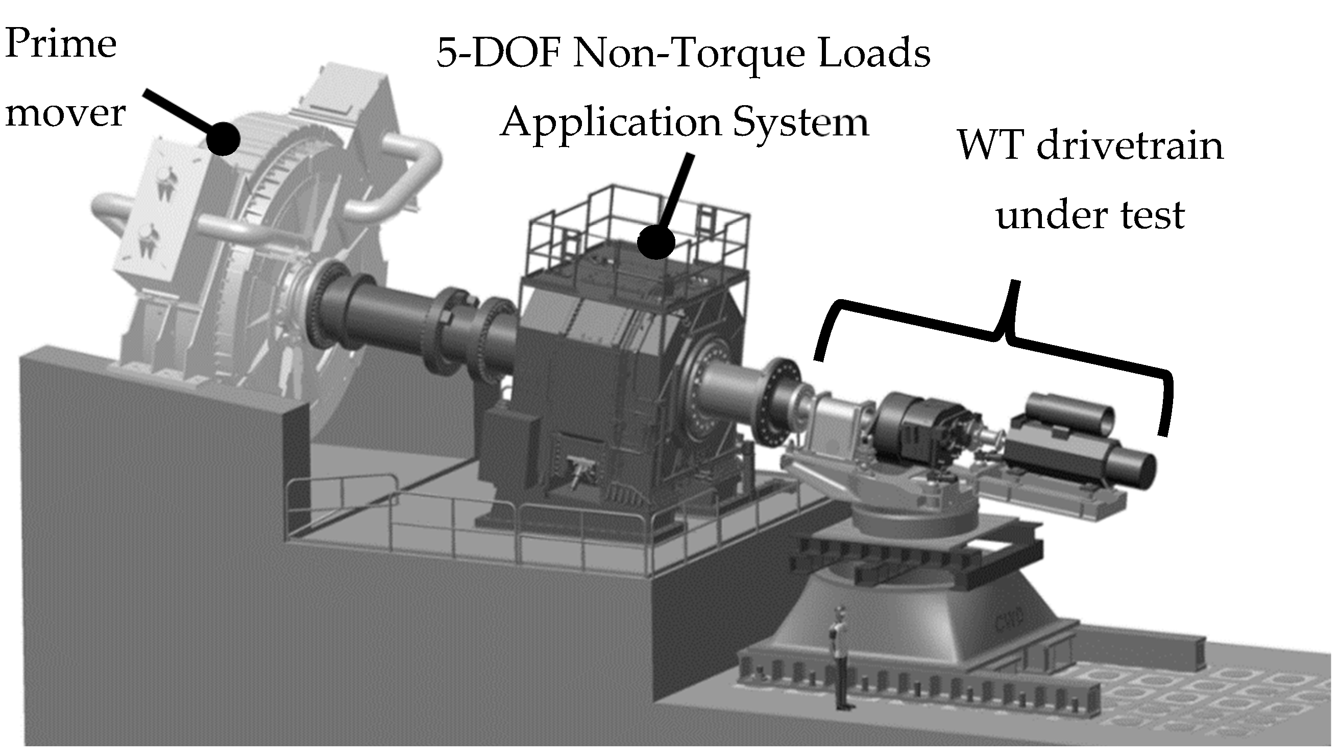
WT system test rigs, such as the one shown in Figure 2, allow investigators to subject a WT drivetrain to different combinations of the loads it is expected to experience during its lifetime in a controlled environment. By instrumenting the WT drivetrain components under investigation, experiments can be designed to capture the responses of interest and the behavior of the system as it experiences the applied loading conditions. Since such tests are resource-intensive, the different combinations of loads can be applied in quick succession in so-called accelerated tests [33], taking Fisher’s famous analogy further from a “questionnaire” [34] (p. 511) for nature to answer to a quick round of Q&A. Accelerated tests generally fall in three categories, which are differentiated by their respective aim: overstressing, increasing usage rates, and tightening the failure threshold [35]. The choice of category depends on the purpose of the experiment. For a more in depth discussion of accelerated tests, Chang et al. provide a selection of highly relevant resources [36]: Chapter 7 of Yang [35], Chapter 6 of Elsayed [37], and Chapters 18 and 19 of Meeker et al. [38]. In order to design accelerated tests that efficiently cover the design space, data from targeted WT simulations are analyzed in this investigation. Using a binning process designed during this investigation to identify factor levels and combinations thereof, this paper presents a method for generating the desired test series. The method achieves this goal by combining multivariate analysis of simulated data with fundamental DOE techniques, such as randomization and replication. As can be seen in Figure 1a, an infinite number of factor combinations can be selected within the continuous design space. Therefore, factor levels are typically chosen to span the range of each respective factor with discrete levels along its range [39]. The goal is to selectively and objectively sample the design space of interest in a sparse manner [40]. Figure 1b illustrates a design space of three factors with five factor levels spanning the range of each factor. As the names imply, randomization refers to the practice of randomly ordering the planned experiments while replication refers to the practice of repeating the planned experiments [16,41]. Randomization provides a line of defense against systemic bias due to unplanned changes in nonexperimental factors, while replication allows for an assessment of the generalization of the conclusions made as it shows how consistent the findings are over multiple identically designed experiments [41,42].
This investigation aims to design experiments covering the realistic regions of the design space of the factors that a Vestas V52 WT can be expected to experience during operation. In this investigation, the experiments are designed in preparation for a measurement campaign to be performed on a purposely instrumented V52 drivetrain using a WT system test rig, as illustrated in Figure 2, where the factors can be controllably applied to the drivetrain. As previously introduced, the purpose of the campaign is to collect real world data for the development of a virtual 6-DOF gearbox (GB) input loads sensing solution. The responses, or dependent variables, in the planned experiments are the signals from a sensor set up primarily applied to the GB housing and consisting of stationary, non-rotating sensors for a more feasible estimation of the 6-DOF GB input loads during WT operation. As demonstrated by Figure 1, the design space and the resulting experiments highly depend on the chosen ranges for the respective factors. Additionally, the fact that the number of factors in this investigation is seven means that the number of needed experiments to perform a full factorial DOE would exponentially grow. In a full factorial DOE without replication, the number of experiments would be the selected number of factor levels the power of seven, which could result in an unfeasibly high number of experiments. Figure 1 also demonstrates a different issue that requires limiting the combinations of factor levels to realistic load combinations. A challenge remains to avoid a premature end to the planned experiments by applying loading combinations in regions of the design space that are unrealistic and therefore unsustainable for the experimental unit. For example, an experiment with all loads set to their respective maximum values would subject the WT drivetrain to an unrealistic and unsustainable load situation, which it was not designed to handle and therefore can cause a costly failure during testing. Hence, a need exists to identify realistic ranges and combinations of loads that a WT drivetrain can be expected to experience in its lifetime and to design time-efficient experiments that cover these load combinations during targeted tests. The methodology presented in this investigation tackles this challenge by aiming to identify and target realistic regions of the design space on the basis of purposely developed computer simulations.
In this investigation, this need is addressed by analyzing simulated time-series data generated from targeted aeroelastic multibody simulations (MBS) of a WT undergoing wind conditions that cover design load cases (DLC) based on the IEC 61400-1 standard [43]. The standard provides guidelines to certify each installed wind turbine according to its predicted response to a variety of operational conditions, which are categorized into DLCs [44]. The simulated time-series data is analyzed to identify the ranges and combinations of the factors that are expected to take place during the lifetime of the WT under investigation. In this work, the Vestas V52 is the WT under investigation due to the availability of a V52 drivetrain for subsequent testing. In a previous investigation, Azzam et al. assembled an MBS WT model of the Vestas V52 and subjected it to simulated wind fields based on DLCs for the purpose of generating simulated data to develop a prototype of a virtual 6-DOF GB input loads sensor [12]. The investigation presented a methodology for generating a simulated time-series of the target variables, 6-DOF GB input loads, as well as the predictor variables, the simulated deformations, misalignments, and rotational speeds of various drivetrain components [12]. Since Azzam et al. aimed to develop the envisaged virtual sensor in the absence of real world data, it was necessary to model and simulate the predictor variables, or the ideal responses of the sensor signals to be expected in the real world. The current investigation, on the other hand, aims to design experiments for a purpose built test rig where it is only necessary to control the applied loads to a purposely instrumented V52 drivetrain in order to collect the true sensor signals. In addition, due to the need for identifying the range of loads that are expected to be experienced by the V52 drivetrain during its lifetime, it is necessary to perform simulations covering a large number of DLCs. Therefore, the current investigation utilizes a simplified variant of the modeling approach demonstrated by Azzam et al., which is more targeted to generate the independent variables, or factors, of the planned experiments, which are the 6-DOF rotor loads and rotational speed. This paper presents a methodology for further processing the resulting time-series data of the target factors from the various DLC simulations to generate a series of designed experiments designed to subject the V52 drivetrain to realistic factor combinations during the planned campaign.
In brief, this investigation aims to provide a methodology to enable investigators to avoid the unmanageable, e.g., unrealistic load combinations or number of planned experiments, and manage the unavoidable, e.g., systemic bias and the need to identify and cover the realistic regions of the design space, when designing tests for a WT drivetrain that require covering realistic combinations of the 6-DOF rotor loads and rotational speed. This is achieved by first outlining a process for generating simulated time-series data of a WT experiencing wind fields covering the design load cases (DLC) according to the IEC 61400-1 [43] in a simulated environment and then presenting an approach for analyzing this data to generate designed experiments that cover the relevant regions of the design space at hand.
The paper is organized as follows. Section 1 introduces and motivates the methods used in this investigation. Section 2 details the proposed methodology with Section 2.1 presenting the modeling and simulation approach and Section 2.2 providing a description of the resulting simulated data. Section 2.3 presents the data analysis. Section 2.4 elaborates on considerations and challenges in practical implementation of the proposed method. Section 3 presents the results of the investigation followed by a discussion of the results in Section 4. The conclusions are then outlined in Section 5.

2. Methods

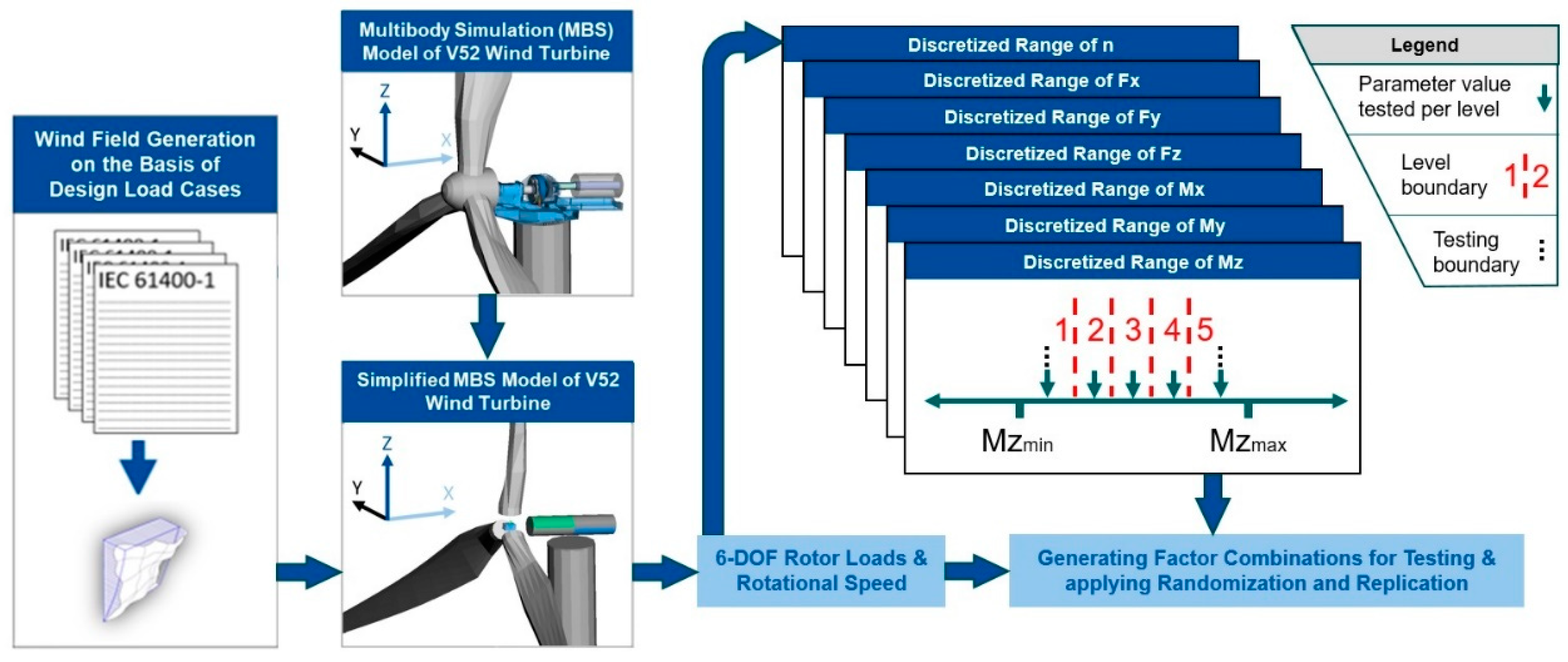
The proposed methodology relies on the efficient implementation of aeroelastic WT MBS simulations and the purposeful analysis of the resulting simulated data to reach realistic accelerated test series covering the experimental design space, while profiting from DOE principles. Figure 3 provides an overview of the simulation and data analysis steps leading to the targeted factor combinations that can be applied to the V52 drivetrain during testing. Figure 3 also indicates the orientations of the x, y, and z axes with respect to the WT drivetrain, which will be followed throughout this paper. Further, Table 1 details the factors as well as clarifies the factor IDs that are used in Figure 3 and will be used herein after to refer the respective factor.
As shown in Figure 3, the proposed method to identify realistic factor combinations, in this case 6-DOF rotor loads and rotational speed combinations, begins with the implementations of simulated wind fields covering a variety of DLCs according to the IEC 61400-1 standard [43]. This step is followed by the application of the simulated wind fields to an MBS model of the WT under investigation, Vestas V52 in this case, in the virtual environment. To clarify the WT models illustrated in Figure 3, Table 2 lists the main specifications of the Vestas V52 WT on which the MBS WT models are based. The drivetrain of the WT model is simplified since the inertia and stiffness of the drivetrain represents its main impact on the rotor loads. This simplification allows for a significant decrease in computational cost and therefore speed, which is needed to cover a large variety of DLCs and provide a more complete picture of the factor combinations that are to be expected during the lifetime of the WT. Section 2.1 details the simulation approach followed in this investigation. The resulting simulated time-series of the factors are then processed to bin each factor into five levels as indicted in Figure 3 for Mz as an example. Section 2.2 provides a description of the simulated data. The five levels are selected based on the range of values of each respective factor while taking into account the control behavior of the specific combination of the test rig and WT drivetrain at hand. The resulting factor level combinations are then tallied and are used for generating the test series for the planned tests. At this stage, highly frequent load combinations can also be covered in higher level resolution by a process outlined in Section 2.3, which describes the data analysis performed in this investigation. Lastly, Section 2.4 provides an overview of the considerations and challenges to be considered for an effective practical implementation of the proposed method.

2.1. Simulation Approach

In order to generate the simulated factors while lowering the computational cost of the planned simulations, simplifications were implemented to the drivetrain of the WT MBS model used in this investigation. Similar to the approach followed by Azzam et al. [12], a modal decomposition of the rotor blades and the tower was performed after an initial modelling in finite elements [47,48]. Micro-level material flaws were not considered in the simulation [12]. The drivetrain components were modeled as a 2 mass oscillator in order to lower the computational cost of the simulations. This substitute drivetrain model takes the torsional stiffness, mass and inertia of the original WT into account. This ensures correct feedback from the drivetrain to the rotor system and thus the rotor loads. In order to simulate and apply wind fields to the WT model and the controller signals for power control in the MBS virtual environment, the AERODYN force element and a MATLAB SIMULINK PI controller were used as part of a co-simulation [49,50]. Within the controller, modules are implemented to control the pitch angle under different operating conditions, such as during WT normal production, startup, shutdown, and emergency shutdown procedures. The controller automatically triggers such procedures based on the rotational speed and pitch angle of the WT model during the aeroelastic MBS. Since the torque is generally constant in the full load state, a torque controller module follows a set speed-load characteristic in partial loading conditions. Actuator models are also implemented in the control strategy to apply delays in order to accommodate the inertias of the components within the WT mechatronic system. The wind fields were created with TurbSim and IECWind [49,51]. Aside from the aforementioned drivetrain model, this work follows the same simulation approach outlined by Azzam et al. to subject an MBS model of the Vestas V52 WT to simulated wind fields based on DLCs from the IEC 61400-1 standard [43]. For a more in depth explanation of this simulation approach, see [12].
The IEC 61400-1 standard [43] provides requirements for the DLCs that must be considered for the certification of new WTs. The DLCs are typically considered by performing calculations or simulations were the respective conditions are applied to the model of the WT under investigation. The standard also provides minimum criteria for the aeroelastic and mechanical WT model to be used in such calculations or simulations, which are generally met by the model used in this investigation. In this investigation, simulated wind fields covering five out of the eight design conditions from the standard were generated and applied to the model of the Vestas V52 WT during aeroelastic MBS simulations. Design conditions 2, 7, and 8 are not covered as they involve condition monitoring system and grid faults as well as blackout, loss of voltage, and loading conditions arising from transport, assembly, and repairs which are beyond the scope of this investigation [43]. The standard defines a number of DLCs for each design condition as outlined in Table 3, which provides an overview of the requirements set by the standard to cover the design conditions included in this investigation. To complete a given DLC, it is typically needed to generate a number of simulated wind fields with each field covering a target wind speed depending on the WT under investigation. The standard also specifies the point at which wind speed is measured to be at the hub of the WT. Six other wind speeds are of relevance at this stage and they are explained in Table 4. The abbreviations in Table 3 and Table 4 will be used herein after to refer to the respective table item. The wind shear is described according to the appropriate formula in the standard with a height exponent of 0.2 for all DLCs. In addition, no dynamic yawing has been included in the simulations as it is not required by the standard. The values in Table 4 are specific to the WT at hand, which is a Vestas V52 in this case belonging to the wind class Ia. The reference wind speed, or Vref, is defined by the IEC 61400-1 standard depending on the wind class of the WT under investigation. The standard also provides formulas to calculate the 50-year and 1-year return period wind speeds, respectively, based on Vref and the WT hub height. For a more in depth explanation of the design conditions, design load cases, and the wind conditions outlined in Table 3, see [43].
Generally, DLCs can be grouped into two categories, those requiring a turbulent wind field model and those requiring a laminar wind field model. To realize a turbulent wind field model, the standard specifies that six wind fields should be generated per wind speed with the turbulence model in each field simulated using a different random seed. The standard also defines the turbulence model according to the wind class of the WT under investigation. Wind speed ranges, such as the one required for DLC 1.1 from Table 3, are covered in this investigation with increments of 1 m/s. Therefore, as an example, 132 wind fields (22 wind speeds multiplied by six random seeds per wind speed) were generated to cover DLC 1.1 as it requires a turbulent wind field model, normal turbulence model. In this investigation, a total of 552 simulated wind fields were generated and applied the V52 MBS model as part of the aeroelastic simulations performed in this investigation to collect the desired time-series data of the simulated factors, 6-DOF rotor loads and rotational speed.

2.2. Data Description

The seven factors were collected from the time-series aeroelastic simulations covering the aforementioned variety of design conditions and respective DLCs. The collected factors were sampled with a frequency of 200 Hz. The duration of each simulation varied depending on its corresponding DLC. In total, the aeroelastic MBS simulations generated roughly 45 million data points for the seven variables.

2.3. Data Analysis

The primary aim of the data analysis methodology detailed in this section is to process the simulated time-series data of the factors to define their design space and reach realistic factor combinations within the same design space. Additionally, a method for covering frequently occurring factor combinations with a higher resolution is proposed to investigate areas of relatively high interest within the design space in greater detail. Though the method is presented in the context of the current investigation with the aforementioned set of seven factors, it is applicable to other investigations where the number of factors or factor levels is different. Section 2.3.1 and Section 2.3.2 present the process for definition and discretization of the design into factor levels, respectively. Section 2.3.3 introduce a variant of the discretization procedure with the aim to cover factor level combinations of high interest in higher resolution, while Section 2.3.4 explains the repetition and randomization of the generated combinations.

2.3.1. Definition of Design Space

The first step is to define the design space of the factors at hand. Ideally, the design space can be defined by surveying the simulated data to identify the respective minimum and maximum values of each factor. However, special consideration for the control behavior of the specific test rig and WT drivetrain under investigation is needed in the likely case when investigators need to set hard limits to the design space that may not be exceeded during testing. Since the DLCs covered during the simulation phase of the proposed method include extreme wind conditions, the minimum and maximum values of the simulated factors are in turn extreme values. To avoid a high risk of unexpected failure of the experimental unit during testing, it is recommended to not exceed these values. In addition, test bench limitations may also require that the range of one or more factors, and in turn the design space, is reduced to the performance limits of the test bench. As an example, In the case of overshoot when attempting to reach a specific target factor combinations, the desired target loading state may be exceeded as the control system attempts to reach the desired state. Therefore, the authors recommend the definition and utilization of a buffer between the experimental design space, bound by testing boundaries, and the design space defined based on the full ranges of the factors obtained from the simulations. An example of such a buffer is illustrated in Figure 4, where the testing boundaries for Mz are visibly separated, in an exaggerated manner for illustration purposes, from the minimum and maximum values of Mz as obtained from the simulated data, respectively. Once the bounds of the experimental design space have been defined, the definition of factor levels can begin.

2.3.2. Discretization of Design Space and Factor Levels Definition

As discussed in Section 1, the discretization of the design space using factor levels is a common practice in the field of DOE to reach a feasible number of factor combinations while covering the design space. The number of factor levels is also a parameter that investigators can select to better fit the requirements of the investigation at hand. In this investigation, five levels per factor were chosen for several reasons. The ranges of several factors, such as My, Mz, and Fy, reached comparably high magnitudes in both negative and positive values. Due to the presence of asymmetries in the design of a typical WT drivetrain, including that of the Vestas V52, the testing of several points was favorable to not only cover the zero level and the extremities of the range, but also to test at moderate positive and negative values of such factors. Similarly, it was decided to opt for five factor levels for all factors in order to gain an understanding of the drivetrain responses to several moderate load levels in addition to the extreme levels. Figure 4 illustrates the five factor levels of Mz as an example. As discussed earlier, the test boundaries define the extent of each factor in the design space, which is also illustrated in Figure 4. The resulting range of testing for each factor is then evenly split into the desired number of levels, in this case five levels. Factor values that exceed or go below the testing boundaries are assigned to the highest or lowest factor levels, respectively. In other words, the highest and lowest factor levels are bound only one-sidedly by the boundary with the respective adjacent inner level. The factor values within each simulated data point are assigned to a respective factor level via a binning process based on the defined level boundaries. Each value in the available data is binned to the respective factor level containing said value. The following pseudocode, outlined in Algorithm 1, clarifies the algorithm for defining level boundaries for each factor as well as the application of the aforementioned binning process to all simulated data points:
Algorithm 1. Algorithm for binning a given factor into desired number of factor levels in available data set according to desired testing boundaries.
min_test = INPUT(“Define minimum testing boundary”)
max_test = INPUT(“Define maximum testing boundary”)
no_lvl = INPUT(“Define required number of levels”)
lvl_width = (max_test − min_test) / no_lvl

FOR each simulated data point DO
   IF factor < min_test + lvl_width THEN
      factor = 1
   ELSE IF min_test + lvl_width < = factor < min_test + 2 * lvl_width THEN
      factor = 2
   ELSE IF min_test + 2 * lvl_width < = factor < min_test + 3 * lvl_width THEN
      factor = 3
    ⁞
   ELSE IF min_test + (no_lvl − 1) * lvl_width < = factor THEN
      factor = no_lvl
   END IF
END FOR
In the case of high separation between the testing boundaries and the minimum and maximum simulated values of a given factor, it may be favorable to increase the ranges of the inner levels. This is due to the fact that by increasing the aforementioned separation, the number of data points assigned to the outer levels will likely also increase potentially resulting in an imbalance between factor levels where some factors are overly represented. This may or may not be favorable depending on the investigation. In this investigation, it was desired to limit such an imbalance. Therefore, a variation of the binning algorithm, presented in Algorithm 1, is proposed for this case in Algorithm 2.
Algorithm 2. Alternative algorithm for binning a given factor into desired number of factor levels in available data set according to desired testing boundaries.
min_test = INPUT(“Define minimum testing boundary”)
max_test = INPUT(“Define maximum testing boundary”)
no_lvl = INPUT(“Define required number of levels”)
no_increment = 2 * no_lvl − 2
lvl_increment = (max_test − min_test) / no_increment

FOR each simulated data point DO
   IF factor < min_test + 1 * lvl_increment THEN
      factor = 1
   ELSE IF min_test + 1 * lvl_increment < = factor < min_test + 3 * lvl_increment THEN
      factor = 2
   ELSE IF min_test + 3 * lvl_increment < = factor < min_test + 5 * lvl_increment THEN
      factor = 3
     ⁞
   ELSE IF min_test + (no_increment − 1) * lvl_increment < = factor THEN
      factor = no_lvl
   END IF
END FOR
At the end of the process outlined in Algorithm 1, the simulated factors are entirely converted from their original numerical values to the corresponding factor levels. In other words, each data point will now contain a combination of factor levels. The next steps involve identifying the unique factor level combinations resulting from the application of the algorithm in Algorithm 1 or Algorithm 2 to the available dataset and choosing a parameter value to test per factor level. The choice of the parameter value to be tested per factor level can depend on the goals of the investigation utilizing the proposed method. In this investigation, testing the extremities of the range of each factor, and in turn, the extremities of the design space is a goal. Therefore, as shown in Figure 4 for Mz as an example, the testing boundaries for a given factor were selected for the highest and lowest of the five factor levels, respectively. As for the inner factor levels, the midpoint of each factor level along the range of a given factor was selected for testing as also illustrated for the example of Mz in Figure 4. More formally, the pseudocode, outlined in Algorithm 3, clarifies the algorithm used in this investigation to define the parameter value used for testing for each factor level. The resulting factor level combinations are then added to the planned test series.
Algorithm 3. Algorithm for defining the parameter value used for testing for each factor level.
min_test = INPUT(“Define minimum testing boundary”)
max_test = INPUT(“Define maximum testing boundary”)
no_lvl = INPUT(“Define required number of levels”)
no_increment = 2 * no_lvl − 2
lvl_increment = (max_test − min_test) / no_increment

FOR each unique factor level combination DO
   IF factor == 1 THEN
      factor = min_test + 0 * lvl_increment
   ELSE IF factor == 2 THEN
      factor = min_test + 2 * lvl_increment
   ELSE IF factor == 3 THEN
      factor = min_test + 4 * lvl_increment
     ⁞
   ELSE IF factor == no_lvl THEN
      factor = min_test + no_increment * lvl_increment
   END IF
END FOR

2.3.3. Procedure for Factor Level Combinations of High Interest

The need may also exist, as is the case in this investigation, to dedicate more tests to cover certain factor level combinations of high interest with higher resolution, i.e., smaller bins, than what is offered by the aforementioned procedure. Therefore, an additional procedure is proposed to cover those factor level combinations.
In this investigation, high interest combinations are defined as those with the highest frequency of occurrence in the available data. More specifically, a threshold has been defined to collect the most frequent factor level combinations collectively accounting for at least 80% of the available data. Thus, the frequency of all unique factor level combinations in the data are first tallied and then the unique combinations are ordered according to their respective frequencies of occurrence. The frequency of each combination is then compared to the total number of data points available to reach the percentage of data points represented by each unique combination. The most frequent unique combinations, collectively representing at least 80% of the available data points, are selected for further analysis as they are considered combinations of high interest in this investigation. Other investigations implementing the proposed method may have varying criteria for selecting the combinations of high interest. The wind profile at a specific WT location may also be analyzed to prioritize and give a relatively higher weighing to DLCs that are most frequently occurring at that location. As an example, Cardaun et al. [52] utilized a reference location provided by the German renewable energies act [53] to reach cumulative frequencies of wind speeds for a similar purpose. In turn, the factor level combinations resulting from the simulations associated with those higher weighted DLCs could be considered of relatively high interest..
Once such unique factor level combinations of relatively high interest have been collected, the following procedure can be followed to cover their corresponding regions in the design space with a higher resolution. Each factor level in a given combination is further split into five sub-levels by following the same algorithm outlined in Algorithm 2 with the testing boundaries defined as the boundaries of the factor level at hand, respectively. The unique factor sub-level combinations are similarly also compiled from the resulting factor sub-level level combinations. Then, the algorithm, outlined in Algorithm 3, is also used with the same definition of testing boundaries in order to reach the parameter value for testing based on the assigned factor sub-level, as it is referred to herein after. The resulting factor sub-level combinations are added to the planned test series, and the process is repeated for all high interest combinations in order to cover their respective factor levels at a higher resolution.

2.3.4. Repetition and Randomization

Lastly, each compiled factor level and sub-level combinations is repeated. The order at which the resulting combinations are tested should also be randomized. In this investigation, each combination was repeated once. Investigations utilizing the proposed method are encouraged to implement at least one repetition if resources allow.

2.4. Considerations and Challenges in Practical Implementation

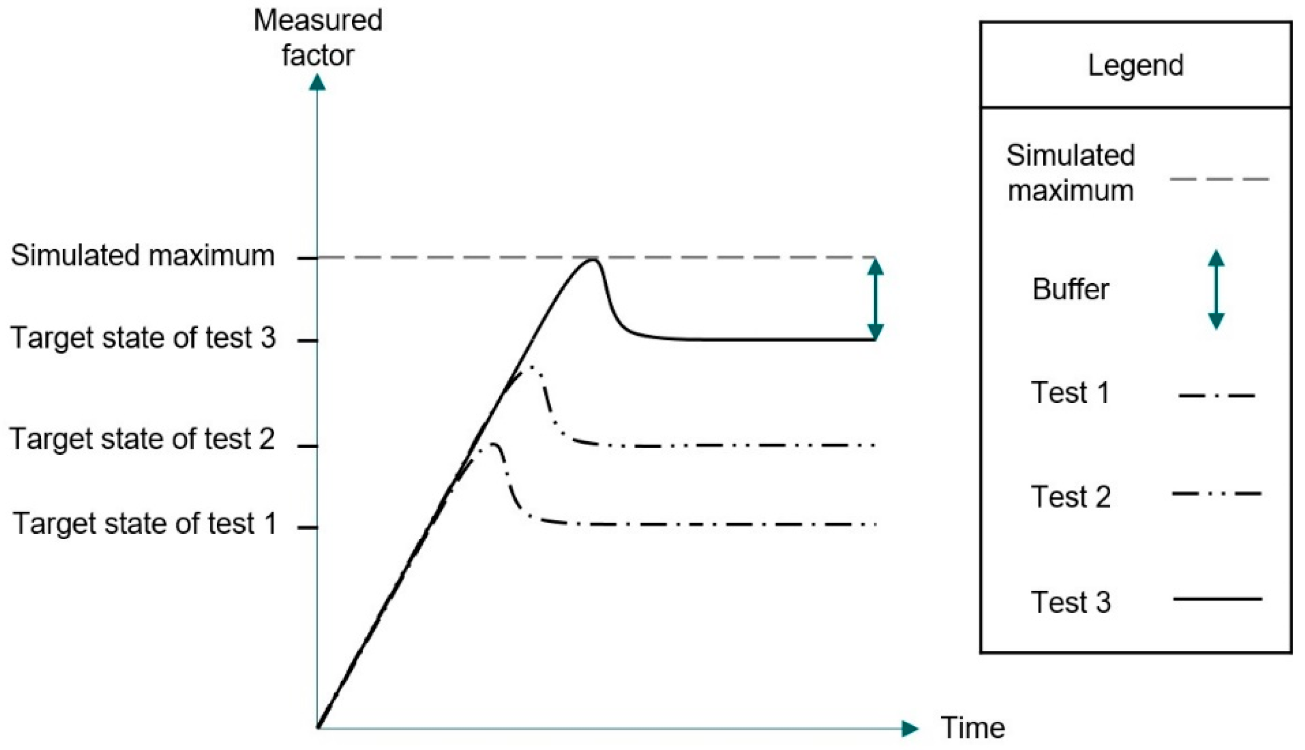
In this investigation, aeroelastic simulations covering a variety of DLCs in accordance with the IEC 61400-1 standard are implemented and the resulting data analyzed to reach realistic rotor loads and rotational speed combinations. The factor combinations are intended to be applied to a purposely instrumented Vestas V52 WT drivetrain using the 4MW WT system test bench, illustrated in Figure 2, with the goal of generating measurement data for the development of a virtual WT 6-DOF transmission loads sensor. The primary motivation for the planned measurement campaign being the absence of field data due to the fact that a practical and cost-effective sensing system has not yet been field deployed. The challenge of validating a WT model in the absence of field data is a common challenge in the wind energy industry. Therefore, the IEC 61400-1 standard [43] provides guidelines for the calculations or simulations of a given WT model subject to the variety of wind conditions that are to be expected during operation, i.e., DLCs. Such guidelines are generally followed by the simulation approach in this investigation. While most experts contest unconditional validity of a simulation model [54,55,56,57], the definition of simulation model validity is possible within the bounds of the project and its intended application [12,58]. Therefore, investigators are encouraged to critically assess the validation requirements of their intended applications of the proposed method, and tailor the fidelity and the comprehensiveness of the model validation approach accordingly. For more considerations and suggestions on the topic of simulation model validity for future applications of the proposed method, see [12] where Azzam et al. introduce and discuss the validity of the initial, higher-fidelity Vestas V52 WT model used in this investigation.
An assessment by the investigators on the validity of the model based on the resulting simulated loads in multiple known simulated wind conditions was deemed sufficient for the purposes of this investigation. Additionally, measures were implemented to mitigate the effects of potential outliers in the simulated data when identifying the bounds of the experimental design space. Domain knowledge was employed to assess the plausibility of the extremes of each factor as well as the ability of the test bench to reach such extremes without exceeding them. As a result, it was decided to separate the testing boundaries from the simulated extremes with a buffer per factor as previously discussed in Section 2.3.1. The magnitude of the buffer is test bench and drivetrain dependent as well as investigation dependent. For example, the rate of change of a given load in order to reach a desired load state typically impacts the degree of overshoot of the system on the way to that state. Therefore, it is recommended to perform initial tests in order to identify the optimal buffer for the investigation at hand. Figure 5 illustrates a simplified example of such set of tests aiming to incrementally reach a definition of a buffer to avoid exceeding the simulated maximum of a single factor due to system overshoot. Figure 5 is also illustrating the often iterative nature of identifying problematic features of the designed experiments and coming up with solutions to mitigate such issues when they arise. For instance, it is often possible to reduce overshoot by reducing the rate of change that would influence the magnitude of the required buffer. However, this will also have an impact on the duration of time needed to cover all designed experiments. Therefore, a tradeoff between the buffer size and the rate of change may exist in this example. Since such a tradeoff would also depend on the available resources to the investigation at hand, identifying the right compromise between these competing testing scenarios may be critical for the realization of the project goals given the available means. These needs and other revelations typically arise during testing and may be difficult if not impossible to fully predict beforehand. Consequently, it is highly recommended to continuously update the computer scripts that generate the desired factor combinations during the testing phase to iteratively fulfill such dynamic needs. Thus, it is also recommended to have flexibility as a design objective when developing those computer scripts in the first place.
The buffer for a given factor in this investigation is chosen depending on the nature of each factor. Hard limits on the bounds of one or more factors are set due to test bench limits. For example, the experiments designed in this investigation are intended for application on the 4 MW WT system test bench illustrated in Figure 2, which is not capable of exceeding an emulated rotor speed of 24 revolutions per minute (rpm). As a result, the testing upper boundary for this factor must be set to 24 rpm in this case. The minimum testing boundary for torque was set to 0 kNm. Some limits are set to avoid permanent damage to the drivetrain under test as such a failure would prematurely end the planned experiments. For example, torque was limited to 440 kNm in order to accommodate a physical safety coupling installed at the gearbox-generator interface as a safety measure to protect the gearbox in the case of the unsustainable application of extreme torque during testing. Similarly, the force Fz was limited to the negative range to avoid drivetrain damage during testing by limiting the maximum testing boundary to the 99th percentile of the simulated Fz loads. Lastly, in order to avoid exceeding the simulated extremes of the applied loads due to overshoot, the testing boundaries of the remaining factors were limited to 90% of the simulated maximum and the simulated minimum values, respectively.
The randomization of factor combinations during testing is useful as discussed in Section 1, however it may also complicate the testing procedures. Depending on the design of the drivetrain under test and the test bench used for load application, clearances within the drivetrain may cause overshoot in situations where the loads are consecutively changed from minimum to maximum values. For example, in the case of the Vestas V52 on the test setup illustrated in Figure 2, extreme changes of Mz would typically cause an overshoot of applied loads due to clearances in the drivetrain components. As such behavior arises during testing, conditionals were put in place to avoid overshoot for every specific case in order to lower the rate of change in specific load transitions as needed, while maintaining higher rates of change when possible to save valuable testing time. For the aforementioned example of Mz when transitioning from extreme positive to negative values, a maneuver was set in place to slow the rate of change considerably before transitioning from negative to positive values and then to recover the normal rate of change for the remainder of the transition. The effort of testing and implementing such strategies during testing increases with randomization as instead of dealing with known load transitions, such as the case with ordered ramps of specific loads, the number of possible transitions is significantly higher. Therefore, it is recommended to consider this practical aspect of randomization when planning resources for the planned experiments and weigh in the benefits of randomization with respect to the available resources and the project goals. Therefore, it is highly recommended to have flexibility as a design objective when developing the computer scripts that generate the test series to enable these changes in the limited time frame of the testing phase.

3. Results

Following the proposed methodology as detailed in Section 2, aeroelastic simulations were conducted on the aforementioned simplified MBS model of the Vestas V52 in order to cover the DLCs listed in Table 3. The minimum and maximum simulated values (in rpm, kN and kNm, respectively) per factor across all simulations are listed in Table 5 along with information on which specific DLC led to each statistic and the time (in seconds) at which each statistic was reached measured since the beginning of each aeroelastic simulation. The times in the table are rounded to the nearest second, while the rotational speeds and 6-DOF loads are rounded to two decimal places. In the table, wind speed refers to the average wind speed (in m/s) of the simulated wind field or, in the case of DLC 6.1, the 50-year return period, which is indicated in the table as 50-year. Yaw in the table refers to yaw misalignment (in degrees) during the simulation. No single simulation generated both the maximum and minimum values of a given factor. In the case of My, two simulations, with different random seeds for the turbulence model, covering the same DLC and wind conditions resulted in both statistics, respectively.
The simulated data was then processed to reach five discrete levels covering the range within the testing boundaries of each respective factor. Table 6 lists the resulting boundaries of the resulting factor levels, while Table 7 lists the parameter values tested at each factor level. As discussed in Section 2, Levels 1 and 5 are only one-sidedly bounded as indicated in Table 6 and they indicate the selected testing boundaries for each of the seven factors in Table 7, respectively. The algorithm detailed in Algorithm 2 was used to bin the simulated data into the factor levels and reach the boundaries listed in Table 6, while the parameter values, listed in Table 7, were defined using the algorithm detailed in Algorithm 3.
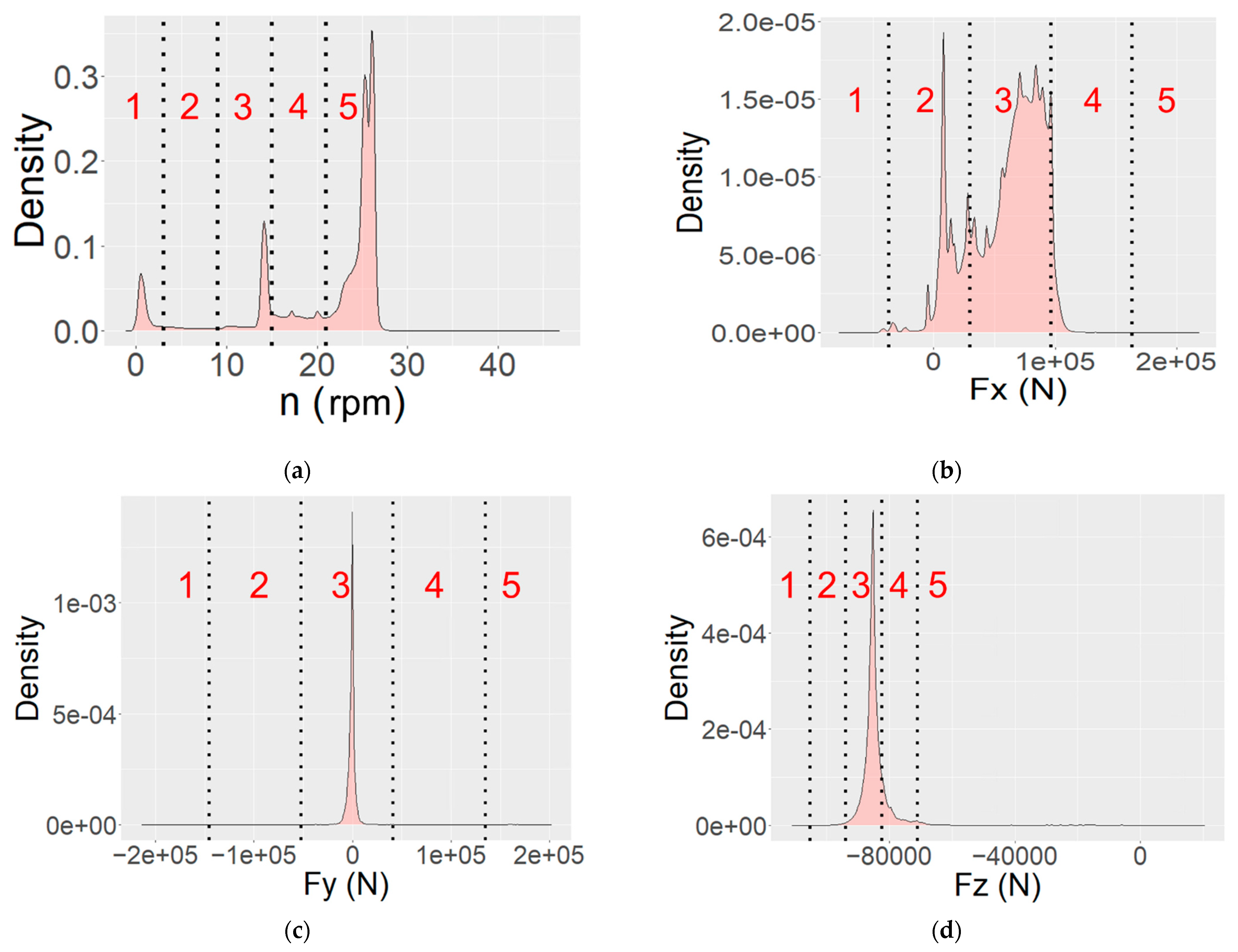
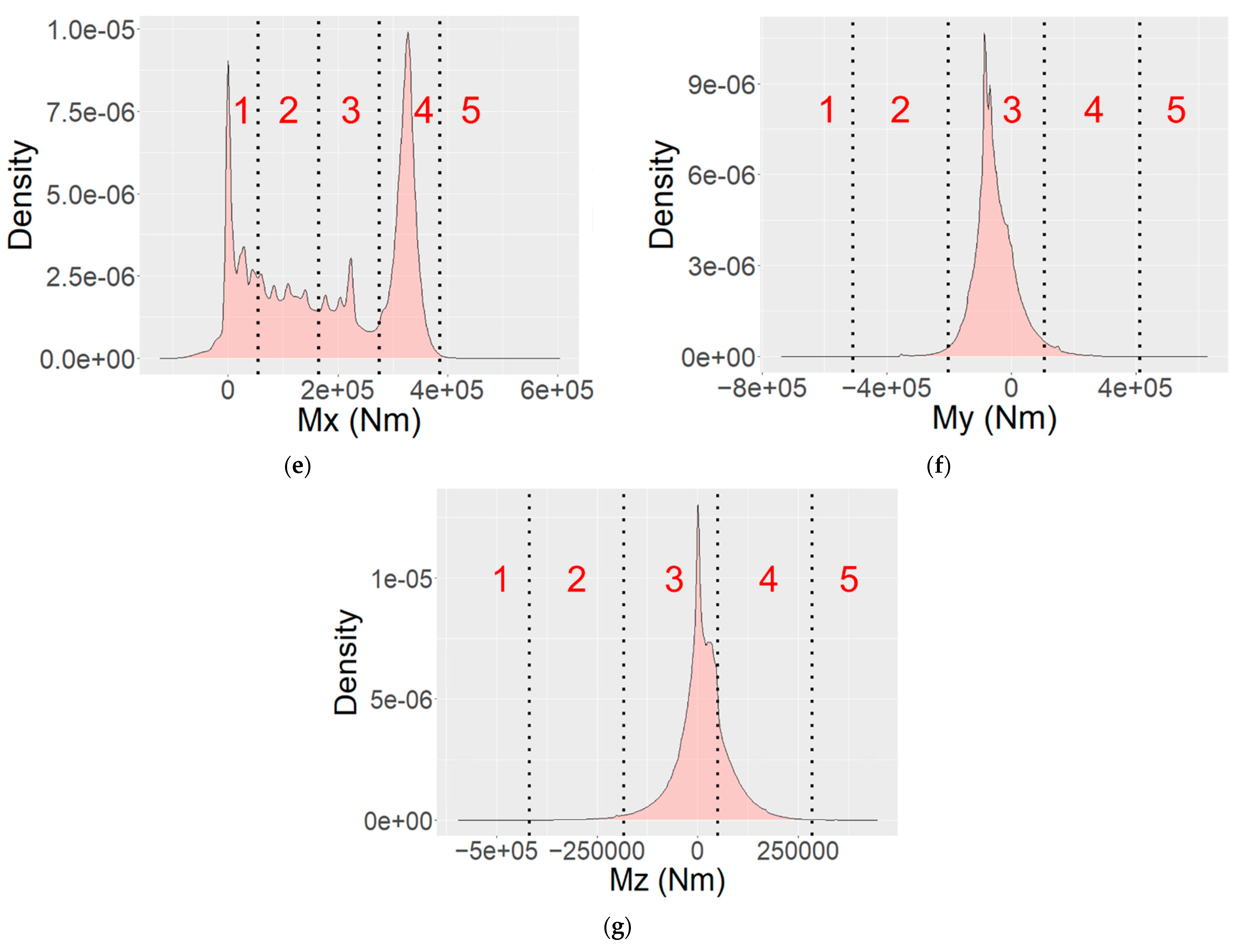
In order to further demonstrate and assess the simulation results as well as factor levels, the distributions of the respective factor levels for each of the seven factors are shown in Figure 6.
Following the methodology outlined in Section 2.3.2, a total of 725 unique factor level combinations were identified. In addition, as discussed in Section 2.3.3, a threshold has been defined to collect the most frequent factor level combinations collectively accounting for at least 80% of the available data resulting in 12 factor level combinations of high interest, listed in Table 8. These combinations led to 2064 unique factor sub-level combinations. In total, 2789 unique combinations were generated.

4. Discussion

The results of the first implementation of the proposed method indicate its high potential in identifying a relatively limited number of factor combinations that cover the realistic regions of the experimental design space. In addition to defining the design space for the given methods, the proposed method generated factor level combinations that cover the regions of the design space that are likely to be experienced by the turbine during operation based on the guidelines of the relevant standard, IEC 61400-1 [43]. In comparison to a full factorial DOE, which would result in over 78,000 factor level combinations to cover the design space at hand, the proposed method resulted in just under 3000 combinations. Table 5 shows the variety of DLCs that are responsible for reaching the extremities of the respective factor ranges, which in turn define the seven-dimensional design space in this case. This demonstrates the utility of performing several simulations in compliance with the IEC 61400-1 standard in order to reach a more complete definition of the design space for the planned experiments. The proposed method also generated level boundaries that split the majority of data points into even factor levels as listed in Table 6. In Figure 6, the proposed algorithms set level boundaries that clearly target the majority of the data points by generating a higher density of factor levels at the more populated regions of the distribution, while being robust against extreme, rare values, such as the extreme maximum value of Fz in Figure 6d. In turn, the proposed algorithms result in the parameter values to be tested at each factor level as listed in Table 7, which also take place with higher density at the more heavily populated regions of the respective factor range as shown in Figure 6. Additionally visible in Figure 6, a common observation among the majority of the factors, such as n, Fy, Fz, My, and Mz, is that a single peak significantly higher than the other peaks in a given factor distribution tends to be entirely or mostly within a single factor level. This is also visible in Table 8, which lists the most frequent combinations collectively accounting for 80% of the data. In the table, it can be seen that for the majority of factors a single level mainly dominates each factor across the 12 combinations. By splitting those dominant factors in the most frequent combinations, the proposed method further demonstrates its effectiveness in selectively targeting the most realistic regions of the design space that the WT at hand can be expected to encounter across all covered DLCs. Therefore, the results demonstrate that the proposed method is successful in achieving the intended goals of targeting the expected combinations of the WT rotor 6-DOF loads and rotational speed.

5. Conclusions

In this investigation, a method is developed to enable investigators to design efficient experiments for testing a WT drivetrain using a WT system test rig by applying realistic combinations of rotor 6-DOF loads and rotational speeds. The main conclusions are as follow:
  • Targeted aeroelastic multibody simulations covering different wind conditions based on the DLCs provided within the IEC 61400-1 standard can be implemented using the developed method to generate simulated time-series data of the 6-DOF rotor loads and rotational speeds that a WT is likely to experience during its lifetime;
  • Simulated data can be analyzed using the developed method to define the design space of the factors under study as well as to reach realistic factor level combinations within the design space to lower the risk of premature drivetrain failure during testing;
  • The proposed method can significantly limit the number of designed experiments as compared to a full factorial design, while targeting highly frequent load combinations at a greater resolution;
  • Due to the promising results achieved using the presented methodology, the authors aim to utilize it in upcoming tests on the drivetrain a Vestas V52 using a WT system test bench capable of applying the generated factor combinations.

Author Contributions

Conceptualization, B.A., R.S. and M.C.; data curation, B.A. and M.C.; formal analysis, B.A. and M.C.; funding acquisition, R.S. and G.J.; investigation, B.A., R.S. and M.C.; methodology, B.A. and M.C.; project administration, B.A. and R.S.; resources, R.S. and G.J.; software, B.A. and M.C.; supervision, R.S.; validation, B.A., R.S. and M.C.; visualization, B.A. and M.C.; writing—original draft, B.A. and M.C.; writing—review and editing, B.A., R.S. and M.C. All authors have read and agreed to the published version of the manuscript.

Funding

This research was funded by the German Federal Ministry for Economic Affairs and Climate Action (0324325).

Institutional Review Board Statement

Not applicable.

Informed Consent Statement

Not applicable.

Data Availability Statement

The data is not publicly available.

Acknowledgments

The authors would like to acknowledge funding from the German Federal Ministry for Economic Affairs and Climate Action of the Research Project “V6LoadS—Virtual 6DOF Load Sensor for the Determination of the Transmission Input Loads and the Resulting Used Up Service Life”. The authors thank the project partners for the provided insight and expertise, which assisted the research. The insights provided by Jonas Gnauert in the lead up to this investigation are also greatly appreciated.

Conflicts of Interest

The authors declare no conflict of interest.

References

  1. Averous, N.; Stieneker, M.; Kock, S.; Andrei, C.; Helmedag, A.; de Doncker, R.W.; Hameyer, K.; Jacobs, G.; Monti, A. Development of a 4 MW Full-Size Wind-Turbine Test Bench. IEEE J. Emerg. Sel. Top. Power Electron. 2017, 5, 600–609. [Google Scholar] [CrossRef] [Green Version]
  2. Kaven, L.; Frehn, A.; Basler, M.; Jassmann, U.; Röttgers, H.; Konrad, T.; Abel, D.; Monti, A. Impact of Multi-Physics HiL Test Benches on Wind Turbine Certification. Energies 2022, 15, 1336. [Google Scholar] [CrossRef]
  3. Schkoda, R.; Fox, C. Integration of mechanical and electrical hardware for testing full scale wind turbine nacelles. In Proceedings of the 2014 Clemson University Power Systems Conference, Clemson, SC, USA, 11–14 March 2014. [Google Scholar]
  4. Lorentzen, T.; Rasmussen, L. Realistic full scale indoor testing of wind turbine nacelles. In Proceedings of the EWEA Offshore 2015, Copenhagen, Denmark, 10–12 March 2015. [Google Scholar]
  5. Gevorgian, V.; Link, H.; McDade, M.; Mander, A.; Fox, J.; Rigas, N. First International Workshop on Grid Simulator Testing of Wind Turbine Drivetrains: Workshop Proceedings; NREL: Boulder, CO, USA, 2013. [Google Scholar]
  6. Stetco, A.; Dinmohammadi, F.; Zhao, X.; Robu, V.; Flynn, D.; Barnes, M.; Keane, J.; Nenadic, G. Machine learning methods for wind turbine condition monitoring: A review. Renew. Energy 2019, 133, 620–635. [Google Scholar] [CrossRef]
  7. Black, I.; Richmond, M.; Kolios, A. Condition monitoring systems: A systematic literature review on machine-learning methods improving offshore-wind turbine operational management. Int. J. Sustain. Energy 2021, 40, 923–946. [Google Scholar] [CrossRef]
  8. Heinold, K.; Panyam, M.; Bibo, A. Considerations for testing full-scale wind turbine nacelles with hardware-in-the-loop. Forsch Ing. 2021, 85, 601–617. [Google Scholar] [CrossRef]
  9. Jassmann, U.; Reiter, M.; Abel, D. An Innovative Method for Rotor Inertia Emulation at Wind Turbine Test Benches. IFAC-PapersOnLine 2014, 47, 10107–10112. [Google Scholar] [CrossRef] [Green Version]
  10. Reisch, S.; Jacobs, G.; Bosse, D.; Matzke, D. Challenges and opportunities of full size nacelle testing of wind turbine generators. In Proceedings of the JSME International Conference on Motion and Power Transmissions, Kyoto, Japan, 28 February–3 March 2017. [Google Scholar]
  11. Riccobono, A.; Helmedag, A.; Berthold, A.; Averous, N.; De Doncker, R.; Monti, A. Stability and Accuracy Considerations of Power Hardware- in-the-Loop Test Benches for Wind Turbines. IFAC-Pap. 2017, 50, 10977–10984. [Google Scholar] [CrossRef]
  12. Azzam, B.; Schelenz, R.; Roscher, B.; Baseer, A.; Jacobs, G. Development of a wind turbine gearbox virtual load sensor using multibody simulation and artificial neural networks. Forsch Ing. 2021, 85, 241–250. [Google Scholar] [CrossRef]
  13. Liu, X.; Azzam, B.; Harzendorf, F.; Kolb, J.; Schelenz, R.; Hameyer, R.; Jacobs, G. Early stage white etching crack identification using artificial neural networks. Forsch Ing. 2021, 85, 153–163. [Google Scholar] [CrossRef]
  14. Azzam, B.; Schelenz, R.; Jacobs, G. Sensor Screening Methodology for Virtually Sensing Transmission Input Loads of a Wind Turbine Using Machine Learning Techniques and Drivetrain Simulations. Sensors 2022, 22, 3659. [Google Scholar] [CrossRef]
  15. Fisher, R. Statistical Methods for Research Workers; Oliver and Boyd: Edinburgh, UK, 1925. [Google Scholar]
  16. Fisher, R. The Design of Experiments; Oliver and Boyd: Edinburgh, UK, 1935. [Google Scholar]
  17. Niedz, R.; Evens, T. Design of experiments (DOE)—History, concepts, and relevance to in vitro culture. Vitr. Cell. Dev. Biol.-Plant 2016, 52, 547–562. [Google Scholar] [CrossRef]
  18. Bacon, F. The Novum Organum of Sir Francis Bacon, Baron of Verulam, Viscount St. Albans Epitomiz’d, for a Clearer Understanding of his Natural History; Thomas Lee: London, UK, 1676. [Google Scholar]
  19. Schwarz, A. The becoming of the experimental mode. Sci. Stud. 2012, 10, 65–83. [Google Scholar] [CrossRef] [Green Version]
  20. Bacon, F. Instauratio Magna (Novum Organum); Apud J. Billium: London, UK, 1620. [Google Scholar]
  21. Jardine, L.; Silverthorne, M. Francis Bacon: The New Organon; Cambridge University Press: Cambridge, UK, 2000. [Google Scholar]
  22. Salsburg, D. The Lady Tasting Tea; W. H. Freeman and Co.: New York, NY, USA, 2001. [Google Scholar]
  23. Fisher, R. Development of the theory of experimental design. In Proceedings of the International Statistical Conferences, Washington, DC, USA, 6–18 September 1947. [Google Scholar]
  24. Deloach, R. Analysis of variance in the modern design of experiments. In Proceedings of the 48th AIAA Aerospace Sciences Meeting Including the New Horizons Forum and Aerospace Exposition, Orlando, FL, USA, 4–7 January 2010. [Google Scholar]
  25. Montgomery, D. Design and Analysis of Experiments, 8th ed.; John Wiley & Sons, Inc.: Hoboken, NJ, USA, 2013. [Google Scholar]
  26. Cox, D. Planning of Experiments; Wiley: New York, NY, USA, 1958. [Google Scholar]
  27. Steel, R.; Torrie, J. Principles and Procedures of Statistics: A Biometrical Approach, 2nd ed.; McGraw-Hill: New York, NY, USA, 1980. [Google Scholar]
  28. Mead, R. The Design of Experiments; Cambridge University Press: Cambridge, UK, 1988. [Google Scholar]
  29. Hinkelmann, K.; Kempthorne, O. Design and Analysis of Experiments, Vol. I: Introduction to Experimental Design, 3rd ed.; Wiley-Interscience: New York, NY, USA, 2008. [Google Scholar]
  30. Hurlbert, S. Pseudofactorialism, response structures and collective responsibility. Austral Ecol. 2013, 38, 646–663. [Google Scholar] [CrossRef] [Green Version]
  31. Brown, S.; Staff, M.; Lee, R.; Love, J.; Parker, D.; Aves, S.; Howard, T. Design of Experiments Methodology to Build a Multifactorial Statistical Model Describing the Metabolic Interactions of Alcohol Dehydrogenase Isozymes in the Ethanol Biosynthetic Pathway of the Yeast Saccharomyces cerevisiae. ACS Synth. Biol. 2018, 7, 1676–1684. [Google Scholar] [CrossRef] [PubMed]
  32. Kasemiire, A.; Avohou, H.; De Bleye, C.; Sacre, P.-Y.; Dumont, E.; Hubert, P.; Ziemons, E. Design of experiments and design space approaches in the pharmaceutical bioprocess optimization. Eur. J. Pharm. Biopharm. 2021, 166, 144–154. [Google Scholar] [CrossRef] [PubMed]
  33. Nelson, W. An updated bibliography of accelerated test plans. In Proceedings of the 2015 Annual Reliability and Maintainability Symposium (RAMS), Palm Harbor, FL, USA, 26–29 January 2015. [Google Scholar]
  34. Fisher, R. The arrangement of field experiments. J. Minist. Agric. 1926, 33, 503–513. [Google Scholar]
  35. Yang, G. Life Cycle Reliability Engineering; John Wiley & Sons, Inc.: Hoboken, NJ, USA, 2007. [Google Scholar]
  36. Chang, M.-S.; Park, T.-K.; Sung, B.-J.; Choi, B.-O. Life prediction of brazed plate heat exchanger based on several accelerated life test data. J. Mech. Sci. Technol. 2015, 29, 2341–2348. [Google Scholar] [CrossRef]
  37. Elsayed, E. Reliability Engineering; Wiley: Hoboken, NJ, USA, 2012. [Google Scholar]
  38. Meeker, W.; Escobar, L.; Pascual, F. Statistical Methods for Reliability Data, 2nd ed.; Wiley: New York, NY, USA, 2021. [Google Scholar]
  39. Farooq, M.; Nóvoa, H.; Araújo, A.; Tavares, S. An innovative approach for planning and execution of pre-experimental runs for Design of Experiments. Eur. Res. Manag. Bus. Econ. 2016, 22, 155–161. [Google Scholar] [CrossRef] [Green Version]
  40. Gilman, J.; Walls, L.; Bandiera, L.; Menolascina, F. Statistical Design of Experiments for Synthetic Biology. ACS Synth. Biol. 2021, 10, 1–18. [Google Scholar] [CrossRef]
  41. Box, G.; Hunter, J.; Hunter, W. Statistics for Experimenters: Design, Innovation, and Discovery, 2nd ed.; Wiley-Interscience: Hoboken, NJ, USA, 2005. [Google Scholar]
  42. Young, J. Blocking, replication, and randomization—The key to effective experimentation: A case study. Qual. Eng. 1996, 9, 269–277. [Google Scholar] [CrossRef]
  43. International Electrotechnical Commission. IEC 61400-1. Wind Turbines—Part 1: Design Requirements; International Electrotechnical Commission: Geneva, Switzerland, 2019. [Google Scholar]
  44. Roach, S.; Park, S.; Gaertner, E.; Manwell, J.; Lackner, M. Application of the New IEC International Design Standard for Offshore Wind Turbines to a Reference Site in the Massachusetts Offshore Wind Energy Area. J. Phys. Conf. Ser. 2020, 1452, 012038. [Google Scholar] [CrossRef]
  45. Rexroth Bosch Group. Operating Instructions—GPV 306 S2 PG 50HZ 61,9 ONSHORE; Rexroth Bosch Group: Lohr am Main, Germany, 2006. [Google Scholar]
  46. Vestas. General Specification Vestas V52 850 kW 50/60 Hz OptiSpeed®- Wind Turbine; Vestas: Randers, Denmark, 2006. [Google Scholar]
  47. Berroth, J. Einfluss der Stelldynamik der Rotorblätter auf die Lasten der Blattverstellsysteme von Windenergieanlagen; Verlagsgruppe Mainz GmbH: Aachen, Germany, 2017. [Google Scholar]
  48. Craig, R.; Bampton, M. Coupling of Substructures for Dynamic Analysis. AIAA J. 1968, 6, 1313–1319. [Google Scholar] [CrossRef] [Green Version]
  49. Jonkman, B. Turbsim User’s Guide: Version 1.50; Technical Report No. NREL/EL-500-38230; National Renewable Energy Laboratory: Golden, CO, USA, 2009. [Google Scholar]
  50. Bi, L.; Schelenz, R.; Jacobs, G. Dynamic simulation of full-scale nacelle test rig with focus on drivetrain response under emulated loads. In Proceedings of the Conference for Wind Power Drives, Aachen, Germany, 3–4 March 2015. [Google Scholar]
  51. Laino, D. IECWind: A Program to Create IEC Wind Data Files, NWTC Design Codes; National Renewable Energy Laboratory: Golden, CO, USA, 2005. [Google Scholar]
  52. Cardaun, M.; Roscher, B.; Schelenz, R.; Jacobs, G. Analysis of Wind-Turbine Main Bearing Loads Due to Constant Yaw Misalignments over a 20 Years Timespan. Energies 2019, 12, 1768. [Google Scholar] [CrossRef] [Green Version]
  53. Renewable Energy Act of 21 July 2014 (BGBl. I S. 1066), Last Amended by Article 1 of the Act of 17 July 2017 (BGBl. I S. 2532). Available online: http://www.gesetze-im-internet.de/eeg_2014/EEG_2017.pdf (accessed on 21 January 2021).
  54. Sargent, R. Verification and validation of simulation models. In Proceedings of the 2010 Winter Simulation Conference, Baltimore, MD, USA, 5–8 December 2010. [Google Scholar]
  55. Babuska, I.; Oden, T. Verification and validation in computational engineering and science: Basic concepts. Comput. Methods Appl. Mech. Engrg. 2004, 193, 4057–4066. [Google Scholar] [CrossRef]
  56. Law, A. Simulation Modeling and Analysis; McGraw-Hill: New York, NY, USA, 2007. [Google Scholar]
  57. Logan, R.; Nitta, C. Verification & Validation: Process and Levels Leading to Qualitative or Quantitative Validation Statements. SAE Trans. 2004, 113, 804–816. [Google Scholar]
  58. Kutluay, K.; Winner, H. Validation of vehicle dynamics simulation models—A review. Veh. Syst. Dyn. 2014, 52, 186–200. [Google Scholar] [CrossRef]
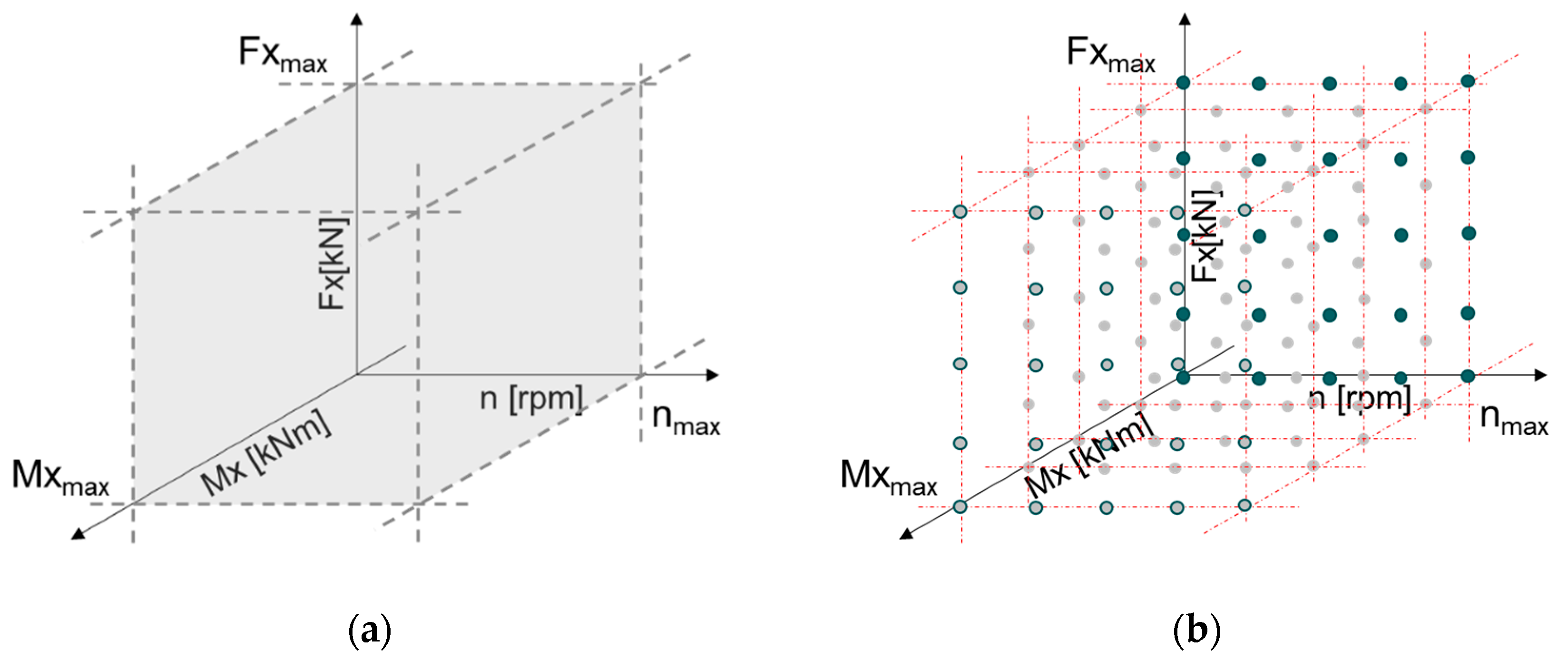
Figure 1. Illustration of an example of: (a) design space for a 3-factor experiment (b) the same design space discretized into five factor levels per factor.
Applsci 13 00356 g001
Figure 2. Illustration of the 4 Megawatt WT system test rig during WT drivetrain testing at the Center for Wind Power Drives in Aachen, Germany.
Applsci 13 00356 g002
Figure 3. Overview of proposed methodology for generation of factor combinations for V52 drivetrain testing.
Applsci 13 00356 g003
Figure 4. Illustration of an example factor range with factor levels and testing boundaries.
Applsci 13 00356 g004
Figure 5. Illustration of a definition of a buffer for a given factor based on system overshoot.
Applsci 13 00356 g005
Figure 6. Simulated distributions and factor levels for each of the respective factors listed in Table 6: (a)–(g) covering factors n, Fx, Fy, Fz, Mx, My, and Mz, respectively, with the respective level number indicated with the red numerals and the respective level boundaries illustrated by the dotted vertical lines.
Applsci 13 00356 g006aApplsci 13 00356 g006b
Table 1. Explanation of experimental factors under investigation.
IDSubject(s)MeasurementAxis of Measurement
MxRotor input loadMomentx
Myy
Mzz
FxRotor input loadForcex
Fyy
Fzz
nRotorRotational speedx
Table 2. Main Specifications of Vestas V52 WT [45,46].
ParameterValues
Rated power850 kW
Wind classIa
Rotor diameter52 m
Rotor maximum speed31.4 rpm
Hub height55 m
Gearbox, typePlanetary and spur
Gearbox, number of stages3
Gearbox ratioi = 61.92
Table 3. Design conditions, design load cases, and implied wind conditions [43].
Design ConditionDLCAmbient Wind ConditionWind Speed(s) 1
1. Production1.1Normal Turbulence ModelVin < Vhub < Vout
1.2
1.3Extreme Turbulence Model
1.4Extreme Coherent gust with change of DirectionVhub = Vr and Vr ± 2 m/s
1.5Extreme Wind ShearVin < Vhub < Vout
3. Startup3.1Normal Wind ProfileVin < Vhub < Vout
3.2Extreme Operating GustVhub = Vin, Vr ± 2 m/s, and Vout
3.3Extreme wind Direction Change
4. Normal shutdown4.1Normal Wind ProfileVin < Vhub < Vout
4.2Extreme Operating GustVhub = Vout and Vr ± 2 m/s
5. Emergency stop5.1Normal Turbulence ModelVhub = Vout and Vr ± 2 m/s
6. Parked (idling)6.1Extreme Wind speed Model50-year return period
6.2
6.31-year return period
6.4Normal Turbulence ModelVhub > 0.7*Vref
1 Explanations are provided in Table 4.
Table 4. Relevant wind speeds specified using the IEC 61400-1 [38] and Vestas V52 datasheet [46].
IDExplanationValue/Source
VhubSpeed at hub of WTDepends on DLC
VinCut-in wind speed4 m/s
VoutCut-out wind speed25 m/s
VrRated wind speed14 m/s
VrefReference wind speed 50 m/s
-50-year return periodFor formula, see [43]
-1-year return periodFor formula, see [43]
Table 5. Factor Statistics from Aeroelastic Multibody Simulations of Vestas V52 WT.
FactorsTime (s)Minimum/
Maximum
Simulated Wind Conditions [43]
DLCWind speed (m/s) Yaw (deg)
n225−1.091.412 0
19646.734.225+4
Fx200−78.054.225−4
200217.974.225−12
Fy100−213.936.150-year+15
161201.376.150-year−15
Fz692−111.041.3250
29720.286.150-year0
Mx161−123.521.4120
198602.724.225+4
My209−737.181.4160
209628.051.4160
Mz158−595.651.4120
337445.881.3250
Table 6. Factor Level Boundaries.
FactorsFactor Value at Level Boundary (rpm, kN, kNm)
1–22–33–44–5
n391521
Fx−36.9429.6696.27162.87
Fy−145.81−52.3741.07134.51
Fz−105.33−93.92−82.50−71.08
Mx55165275385
My−509.87−202.69104.48411.66
Mz−418.91−184.5749.78284.12
Table 7. Parameter values tested at each factor level.
FactorsParameter Values Tested at each Factor Level (rpm, kN, kNm)
12345
n06121824
Fx−70.25−3.6462.97129.57196.18
Fy−192.53−99.09−5.6587.79181.23
Fz−111.04−99.63−88.21−76.79−65.37
Mx0110220330440
My−663.46−356.28−49.11258.07565.25
Mz−536.08−301.74−67.39166.95401.29
Table 8. Most frequent factor level combinations collectively accounting for 80% of available data.
Combination IDFactor Levels
nFxFyFzMxMyMz
15333433
23233133
35333434
45333233
55333333
64333233
71234133
85334433
95333234
105333334
113333133
125433333
Disclaimer/Publisher’s Note: The statements, opinions and data contained in all publications are solely those of the individual author(s) and contributor(s) and not of MDPI and/or the editor(s). MDPI and/or the editor(s) disclaim responsibility for any injury to people or property resulting from any ideas, methods, instructions or products referred to in the content.