Abstract
The pavement deflection measured by falling weight deflectometer (FWD) detection equipment can be used to determine the bearing capacity of a pavement structure through modulus backcalculation to provide suggestions for pavement structure maintenance. However, because asphalt mixtures are temperature-sensitive materials, they are greatly affected by temperature, and changes in temperature can cause their mechanical properties to vary and affect the structural bearing capacity. Therefore, this paper conducts a pavement deflection test on an in-service highway asphalt pavement at different temperatures in different seasons. The representative temperature of the asphalt layer was determined through comparative analysis. The temperature’s effective influence distance on the deflection basin was found, and a more suitable temperature correction model for the deflection basin of asphalt pavement was established. The results showed that the temperature at the middle layer depth of the asphalt layer is more suitable as the representative temperature of the asphalt layer. The effective influence range of temperature on the deflection basin is 90 cm. The deflection change rate before and after the temperature correction at a radial distance of 20 cm is more appropriate for the temperature correction of the deflection basin.
1. Introduction
Falling Weight Deflectometers (FWD) are increasingly being used in pavement maintenance management to determine the structural load-carrying capacity of asphalt pavements by simulating traffic loads to detect surface deflections [1,2]. FWDs have been widely used in assessment of the whole life cycle of pavement structures. For example, during the use of pavement, the backcalculated structural layer modulus based on the deflection basin can be compared with the initial modulus value to determine the structural bearing capacity, thus providing guidance on the best timing for preventive maintenance and the reconstruction and repair of the pavement structure [3,4]. Normally when performing comparative analysis of the initial modulus, it is necessary to correct the backcalculated layer’s modulus to a uniform standard temperature [5].
Deflection is influenced by load factors (applied load size, load bearing plate size), pavement structure (pavement type, number of structural layers, thickness of each layer and structural layer modulus) and asphalt mixture temperature [6,7]. However, asphalt mixtures are temperature-sensitive materials, and both long-term seasonal changes and short-term daily temperature differences can lead to changes in their stiffness [8,9,10]. As the temperature rises, the deflections also increase, and for the same road section, the measured deflections in summer are significantly larger than the deflections detected in winter. When using the deflections to assess the structural performance of pavement, deflections should be corrected for temperature and adjusted to the same reference temperature [11,12]. Then, the corrected deflection can better reflect the structural strength of the pavement by backcalculation. We refer to this temperature correction method as first-correction [13,14]. Usually, the deflections should be normalized at first so that other factors (humidity, asphalt layer damage, asphalt aging, etc.) have minimal influence on the deflection-temperature correction model [15].
To better model the deflection temperature correction, an accurate representative temperature of the pavement should be obtained. The temperature of the asphalt layer varies with depth. For changes in temperature with the depth of the pavement, the temperature’s influence on the stress state is more significant when the pavement’s thickness is deeper. Usually, the temperature at a certain depth is selected to represent the asphalt layer temperature. Different researchers have different opinions on which depth to choose. Baltzer and Stubstad et al. took the temperature of the top third of the asphalt layer as the representative temperature of the asphalt layer and achieved good fitting results [16,17]. Noureldin et al. found that the temperature at near the center of the asphalt layer can represent the actual temperature of the entire asphalt layer [18,19]. Kim and Park investigated the effect of different load magnitudes on the deflection temperature correction factors and obtained a linear relationship between the deflection and the temperature in the middle asphalt layer in semi-logarithmic coordinates [20]. These analyses are mostly based on flexible pavements. However, semi-rigid asphalt pavement is widely used in China. The temperature in the middle asphalt layer is used as a representative temperature in most of the temperature correction model studies [13,21].
Current asphalt pavement temperature prediction models can be divided into two categories: mathematical statistical methods and theoretical methods [22,23,24,25]. The mathematical statistical method refers to the use of the actual measured pavement temperature combined with the meteorological data at that time to determine a pavement temperature calculation formula through regression analysis. The theoretical method derives the expression of the pavement temperature through the principle of heat transfer based on the thermodynamic properties and meteorological data of the pavement material. Comparing the two methods, the mathematical statistics method is relatively simple, while the theoretical method is too complicated. Although the mathematical statistics method has certain regional characteristics, it is still effective for regions with similar climates.
In summary, modulus backcalculation based on FWD deflection is an important part of pavement structure maintenance, and an accurate backcalculation of the asphalt layer modulus is affected by the temperature-sensitive characteristics of the asphalt mixtures. However, a uniform deflection temperature correction model for semi-rigid asphalt pavements has not been fully developed.
Therefore, in this paper, in order to establish an accurate deflection temperature correction model, continuous deflection tests were performed on in-service highway asphalt pavement in different seasons, and the detected pavement temperature was recorded. Then, the representative temperature of the asphalt layer and the temperature’s effective influence distance on the deflection basin were determined. Finally, a temperature correction model of asphalt pavement deflection based on the deflection change rate was also established.
2. FWD Test
To study the deflection of asphalt pavement under FWD loads and its relationship with the road temperature, as well as to establish the temperature correction relationship of the deflections, this paper selected an in-service highway asphalt pavement with a service life of 12 years in Shanghai province and conducted FWD tests under different temperatures and seasons. The traffic volume is 499 pcu/h. The test section is a semi-rigid base asphalt pavement, and the specific structure is shown in the Table 1.

Table 1.
Pavement structure information.
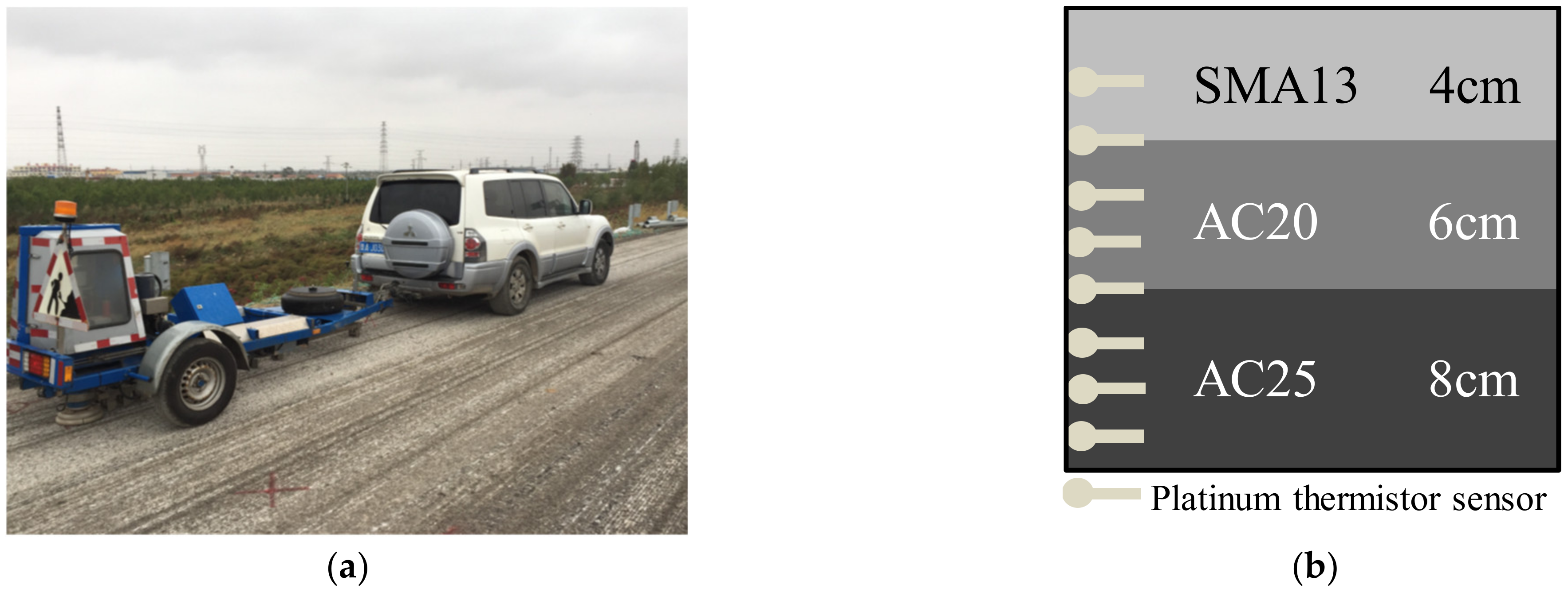
The test section is 1.5 km long and has three lanes in total. Deflection measurement points were arranged in each lane at intervals of 20 m. The measurement points were marked to ensure that each detection was performed at the same location. In principle, the FWD test were to be conducted once a month, but if there is a large temperature difference in that month, two tests were conducted. FWD testing schematic is shown in Figure 1a. The whole test lasted one year. The radial distance of each measurement point is 0, 20, 30, 45, 60, 90, 120, 150 and 180 cm.

Figure 1.
Illustration of the FWD test: (a) FWD testing schematic; (b) Platinum thermistor sensors’ distribution diagram.
To determine the temperature distribution in the structural layer of the asphalt pavement, two temperature monitoring points were arranged in the test road section, and eight platinum thermistor sensors were embedded in each monitoring point, which were buried 2, 4, 6, 8, 10, 12, 14 and 16 cm away from the surface. The platinum thermistor sensors’ distribution diagram is shown in Figure 1b. The temperature of the structural layer was observed throughout the day, with temperature data being collected every 5 min and the prevailing air temperature being recorded at the same time.
3. The Representative Temperature of the Asphalt Layer
3.1. Determining the Representative Temperature
In this paper, to determine the representative temperature of the pavement structure, the temperature at one-third depth and the temperature at the middle depth were adopted as the representative temperatures of the asphalt layer. Then, the surface layer moduli were backcalculated, and the backcalculated modulus and temperature were fitted to compare the fitting effect to choose the appropriate representative temperature.
The backcalculation software used in this study is the SA-PSO program based on the particle swarm algorithm, which has been compared with other backcalculation software such as MODULUS, EVERCALC and WESDEF [26]. The comparison results show that the backcalculation’s accuracy and efficiency are very good.
3.2. Analysis and Results
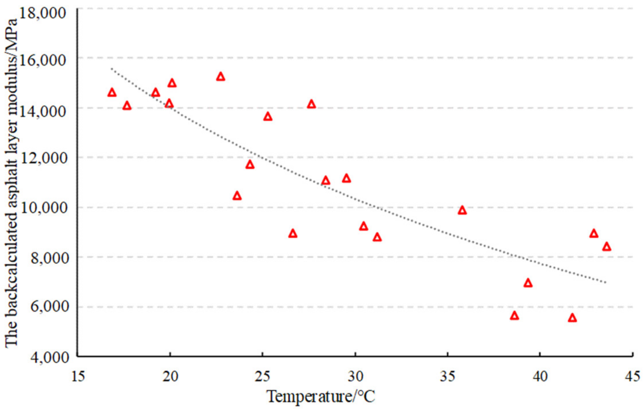
The average modulus of the asphalt layer obtained from the backcalculation was averaged according to the temperature, and the modulus–temperature relationship was modeled by statistical regression. It was found that the logarithm of the modulus is linearly related to temperature, which is shown in Equation (1):
where is the test temperature in °C, is the backcalculation modulus at the test temperature, in MPa, and a and m are different regression coefficients.
Then, the temperature correction coefficient was exponentially related to temperature. Therefore, an exponential relationship model was used to regress the modulus–temperature data, as shown in Equation (2):
where is the standard temperature in °C, is the modulus corrected to the standard temperature, in MPa, and is the correction factor.
When the temperature at one-third depth was used for modeling, the fitted curves and model parameters obtained were shown in Figure 2 and Equation (3):
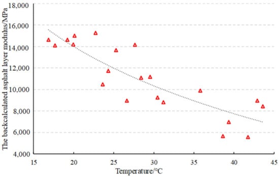
Figure 2.
Modulus–temperature model (at 1/3 depth).
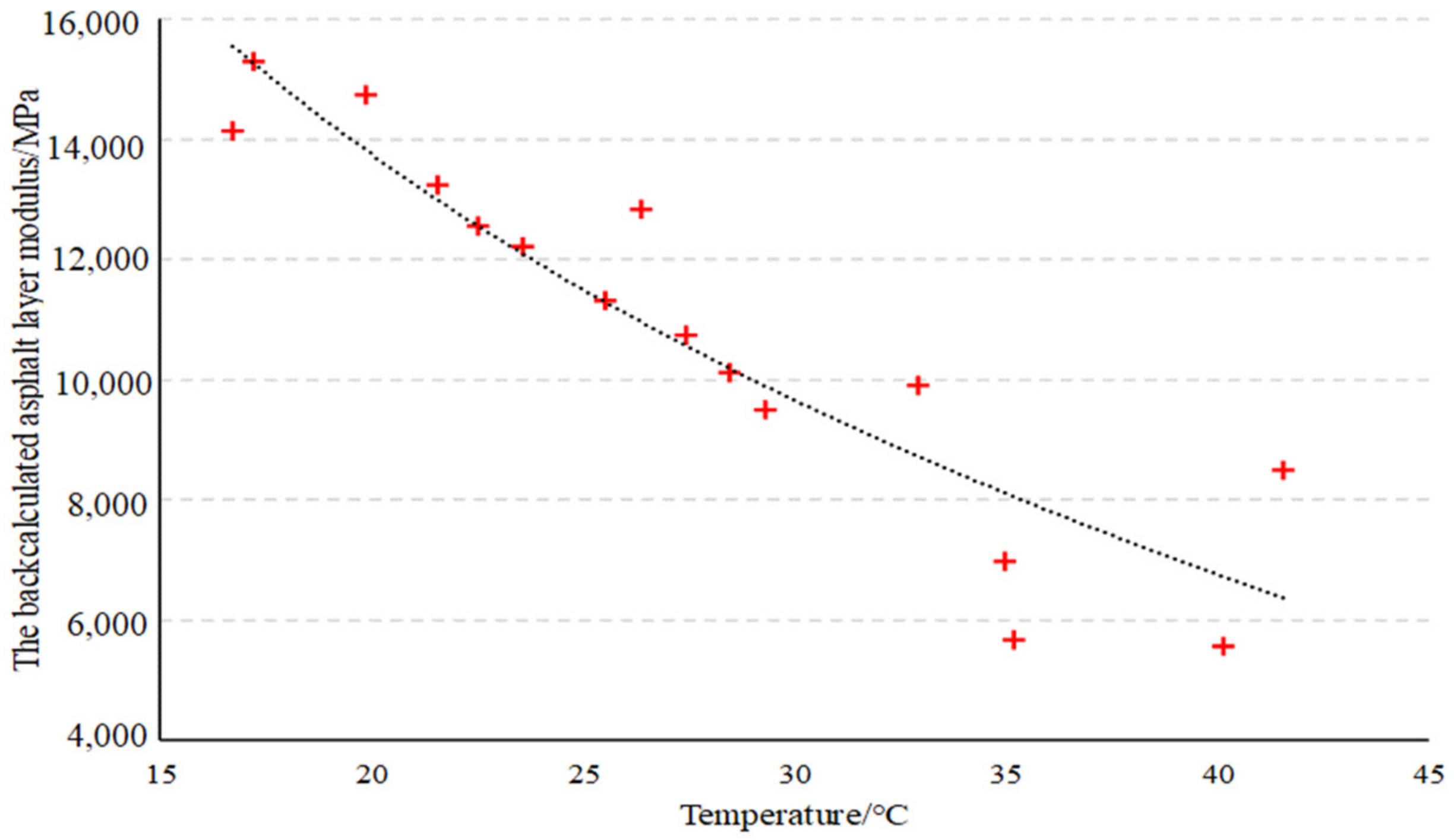
When the temperature at the middle depth was used for modeling, the fitted curves and model parameters obtained were shown in Figure 3 and Equation (4):
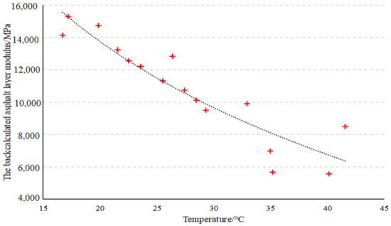
Figure 3.
Modulus–temperature model (at middle depth).
From the above results, it can be seen that both models can achieve a better fitting effect, but in comparison, the fitting curve of R2 is larger and the fitting effect is better when the temperature at the middle depth is chosen as the representative temperature. Therefore, this paper uses the temperature at the middle depth as the representative temperature of the asphalt layer.
4. Effective Influence Distance of Temperature on the Deflection Basin
4.1. Determining the Effective Influence Distance of Temperature
The research shows that the deflection is no longer affected by temperature changes beyond a certain point in the radial distance range, and the distance from this point to the load center is called the effective temperature influence distance. In this section, the collected deflections were first backcalculated for the structural layer moduli, and then the backcalculated surface layer modulus was corrected to 20 °C according to the aforementioned temperature correction model. Next, Bisar software was used to calculate the complete deflection basins using the correct backcalculated surface layer modulus, base layer and subgrade moduli. Finally, the calculated deflection basins were compared with the measured deflection basins to analyze the effective influence distance of temperature on the deflection basin.
4.2. Analysis and Results
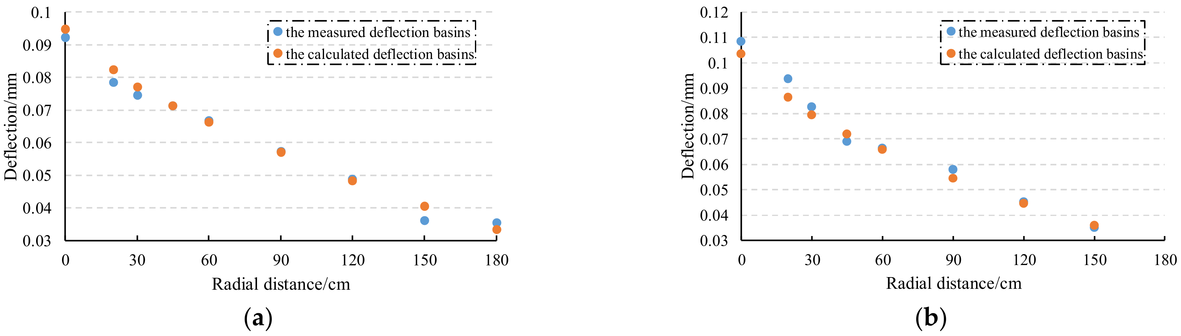
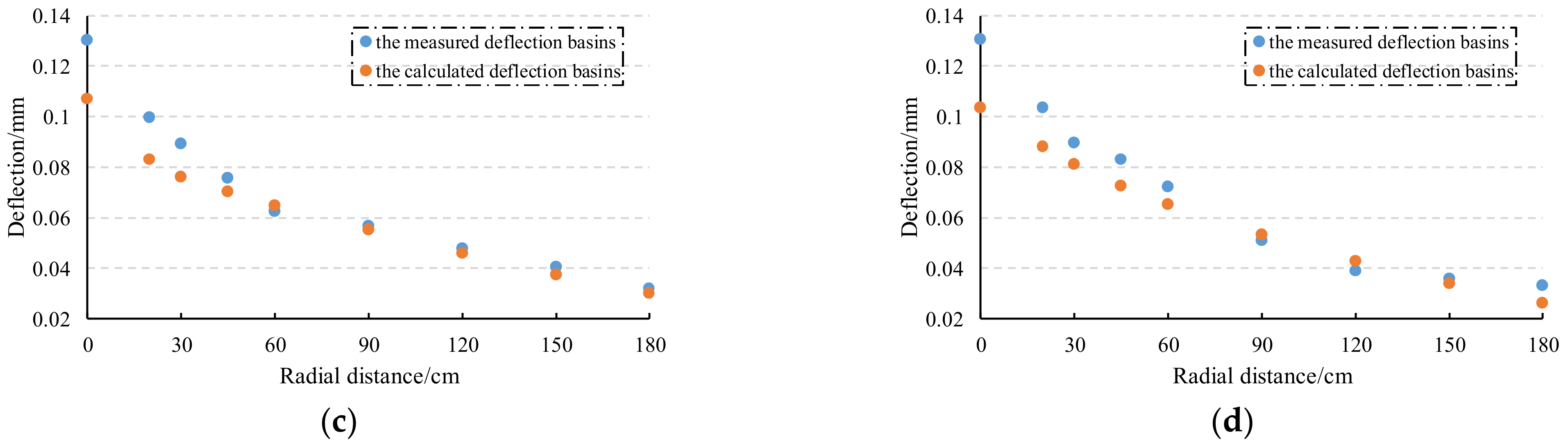
The deflection basins before and after correction under different temperatures at a measurement point were used as an example for analysis which were shown in Figure 4.
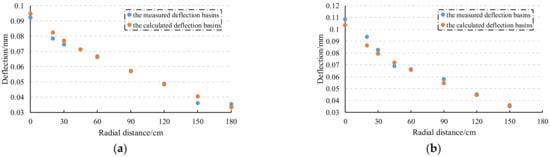
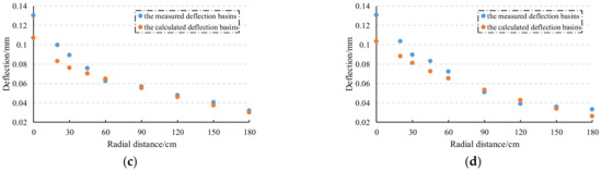
Figure 4.
Comparison of deflection basins at different temperatures: (a) 16.1 °C; (b) 25.1 °C; (c) 35.2 °C; (d) 41.6 °C.
According to the above comparison chart, the influence of temperature on deflection decreases with the increasing radial distance. The deflection difference between the calculated and measured deflections when the radial distance is less than 90 cm is obvious and increases with the increasing temperature difference. However, the deflection differences when the radial distances are farther than 90 cm are not obvious. Then, the difference between the measured and calculated deflection of each measuring point is calculated, and the absolute value of the difference is averaged. The results are shown in Figure 5.
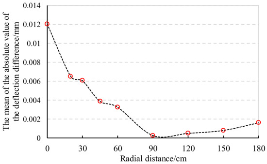
Figure 5.
The mean of the absolute value of the deflection difference.
From the graph of the mean value of the absolute difference between the measured and calculated deflection, the deviation first decreased and then increased and reached a minimum value near the radial distance of 90 cm.
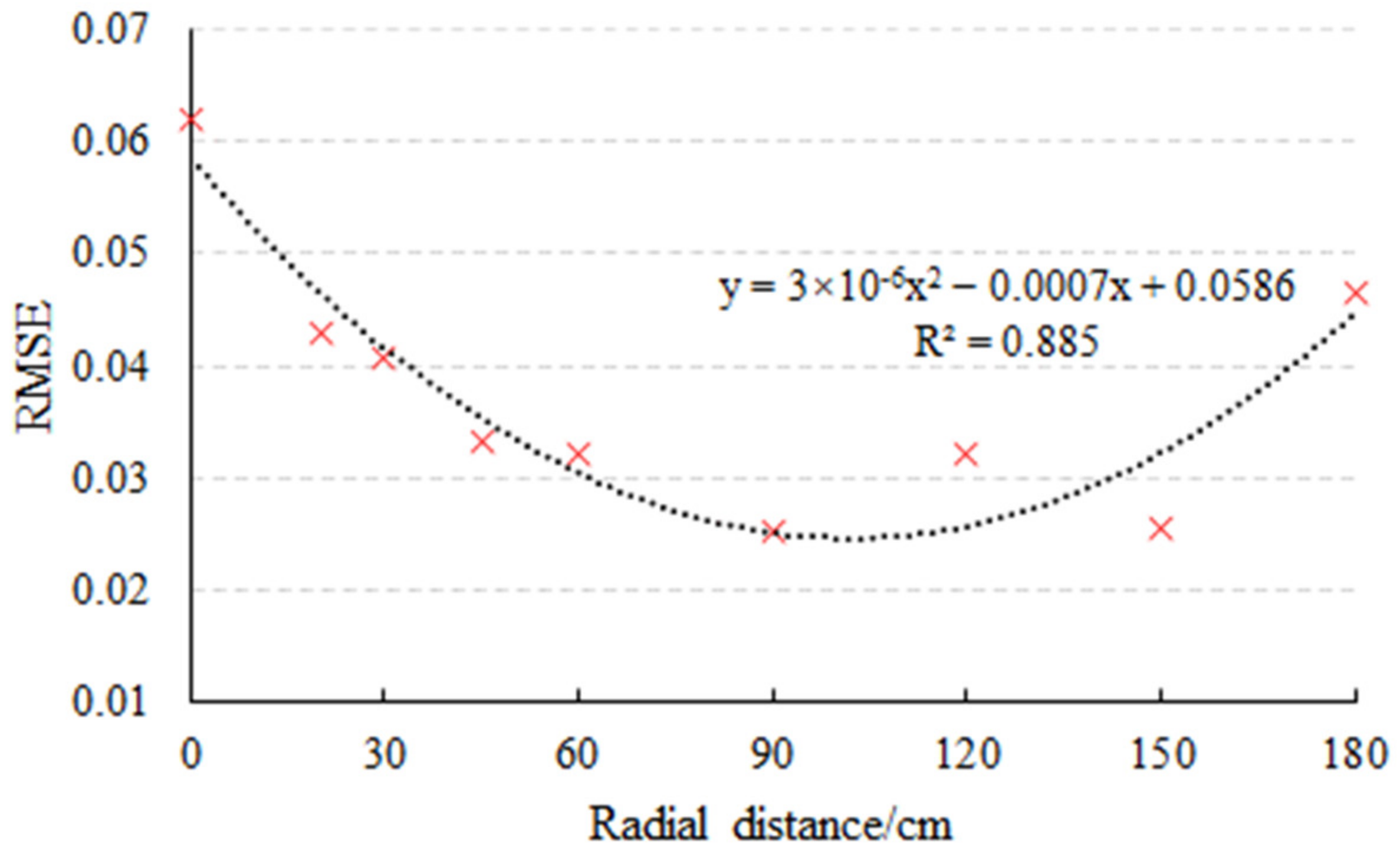
To further verify this conclusion, this paper adopts a method for selecting the effective influence distance based on the minimum mean square error criterion. For the deflection at the same radial distance of a certain measuring point, first calculate the average value of the measured deflections at different test temperatures. Next, calculate the mean value of the measured deflections at different test temperatures with other radial distances. Then, the root mean squared error (RMSE) is calculated by summing the squared differences between the measured deflection and the mean value at different radial distances. The distance between the load center and the point with the smallest RMSE value is the effective influence distance of the structure. The calculation formula of the RMSE is as follows:
where n is the number of different test temperatures selected, is the deflection of the ith test temperature, and is the average value of the different test temperatures from a certain measurement point.
Figure 6 shows that the overall trend of the RMSE first decreases and then increases and reaches the minimum value at 90 cm.
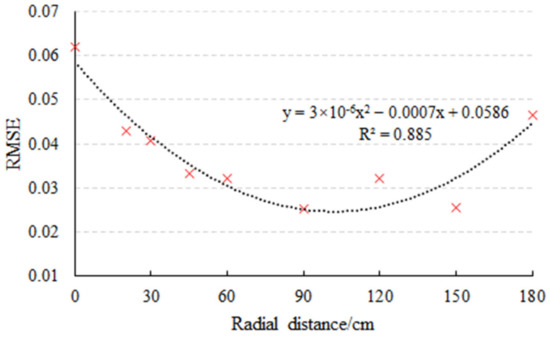
Figure 6.
RMSE at different radial distances.
In summary, it can be determined that the effective radial distance of the temperature on the influence of the deflection basin is 90 cm. The deflections from the load center to the radial distance of 90 cm must be corrected for temperature. The deflection at further radial distances does not require correction.
5. Deflection Temperature Modelling
5.1. Temperature Correction Model at the Load Center
Through the comparative study of the load center deflection under different temperatures, it is found that similarly using the exponential model to correct the load center deflection has a better effect, and the equation is shown below:
where and are deflections at standard and test temperatures, respectively, in mm; is the test temperature, in °C; and is the model parameter.
The fitting results of the load center deflection before and after the correction are shown in Figure 7. The specific temperature correction formula is shown in Equation (7).
where is the temperature correction factor.
Figure 7.
Load center deflection fitting results.
5.2. Temperature Correction Model for the Deflection Basin
In addition to correcting the load center deflection, temperature corrections for deflections are required for other points in the deflection basin that are affected by temperature. This section finds the optimal temperature correction method for deflection at other radial distances by comparing three different temperature correction methods.
5.2.1. Temperature Correction Based on Load Center Deflection Difference
This method looks for the relationship between the difference before and after the temperature correction of deflections at other radial distances and the load center deflection difference based on the difference between the measured load center deflection and the calculated deflection at the load center after modulus correction.
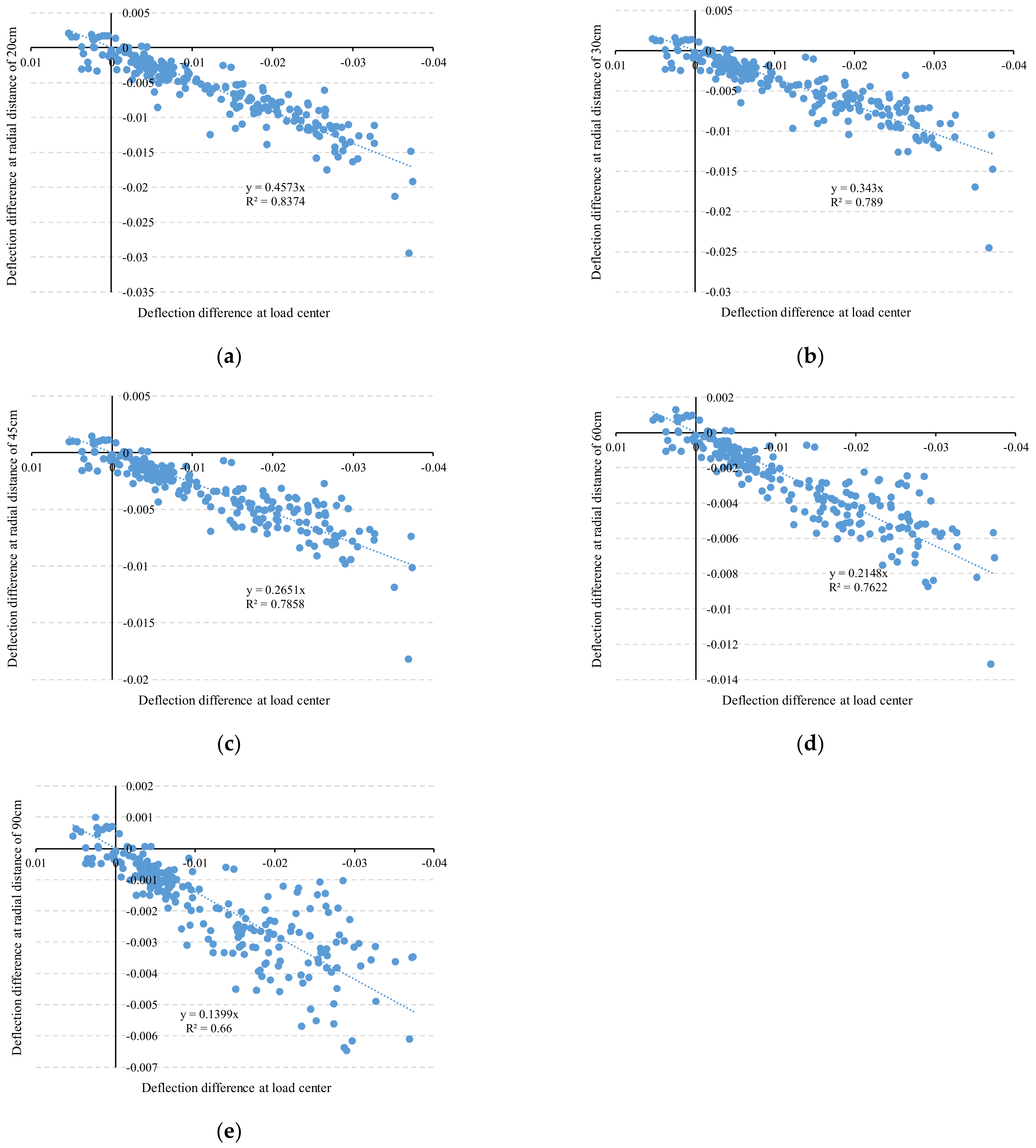
The plots of the deflection difference at the load center and each point at the radial distance from 20 to 90 cm were analyzed, and it was found that there was an obvious linear relationship, so the proportional function was used for fitting. The fitting results at different radial distances are shown in Figure 8. The ratio k and correlation coefficient (R2) of the deflection difference at each point and the load center are obtained, and the results are shown in Table 2.
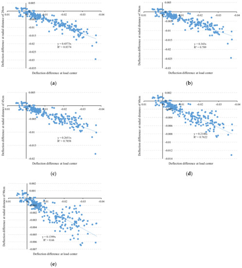
Figure 8.
Fitting results between deflection difference at different radial distances and load center deflection difference: (a) 20 cm; (b) 30 cm; (c) 45 cm; (d) 60 cm; (e) 90 cm.
Table 2.
Adjustment factors for deflection temperature at different radial distances.
Then, the deflection temperature correction model at different radial distances in the temperature-affected range is obtained.
where , , , , and are the temperature-corrected deflections at radial distances of 0, 20, 30, 45, 60 and 90 cm, respectively. , , , , and are the measured deflections at radial distances of 0, 20, 30, 45, 60 and 90 cm, respectively.
5.2.2. Temperature Correction Based on the Load Center Deflection Rate
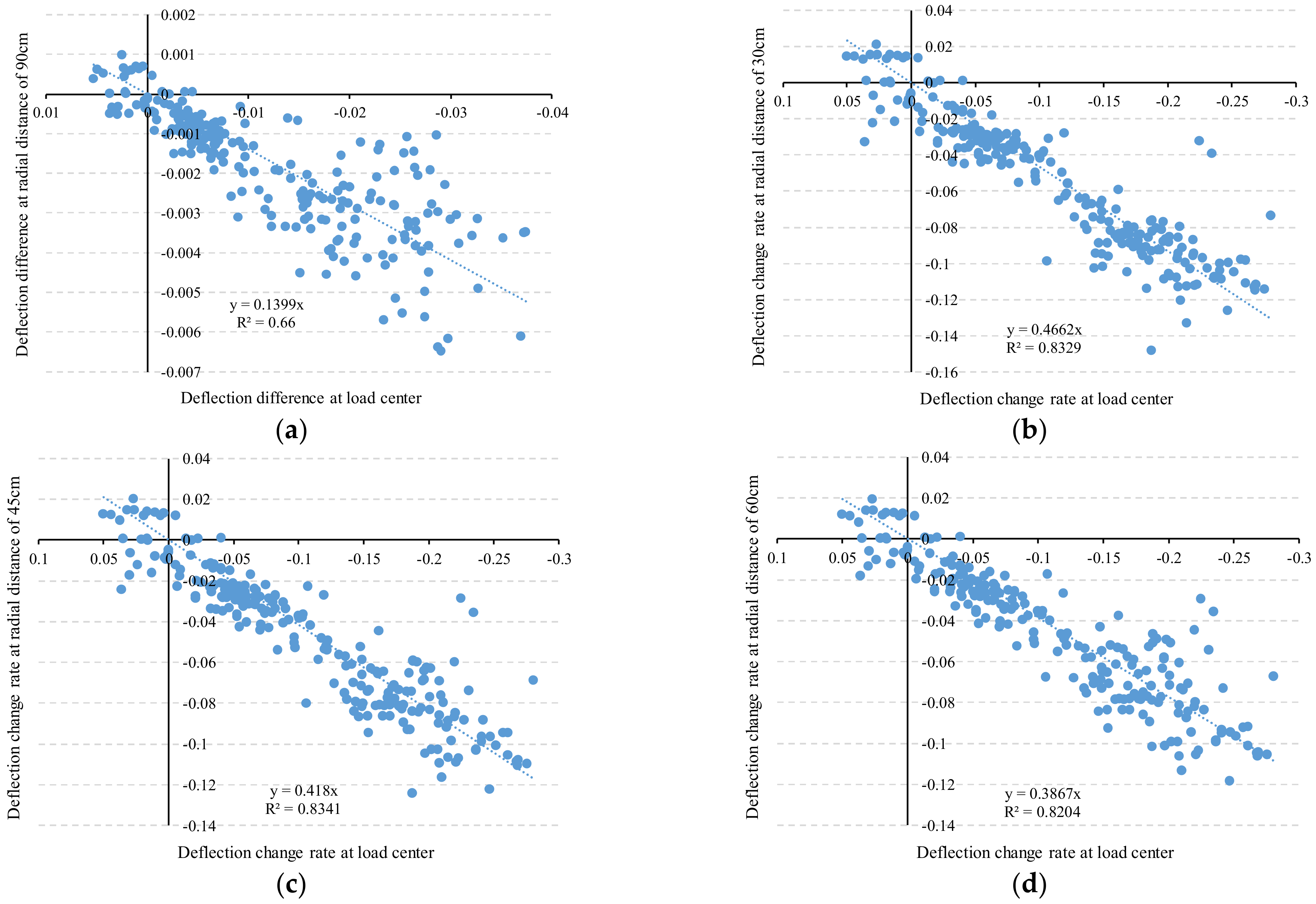
This method looks for the relationship between the change rate before and after the temperature correction of deflections at other radial distances and the load center deflection change rate based on the change rate between the measured load center deflection and the calculated deflection at the load center after modulus correction.
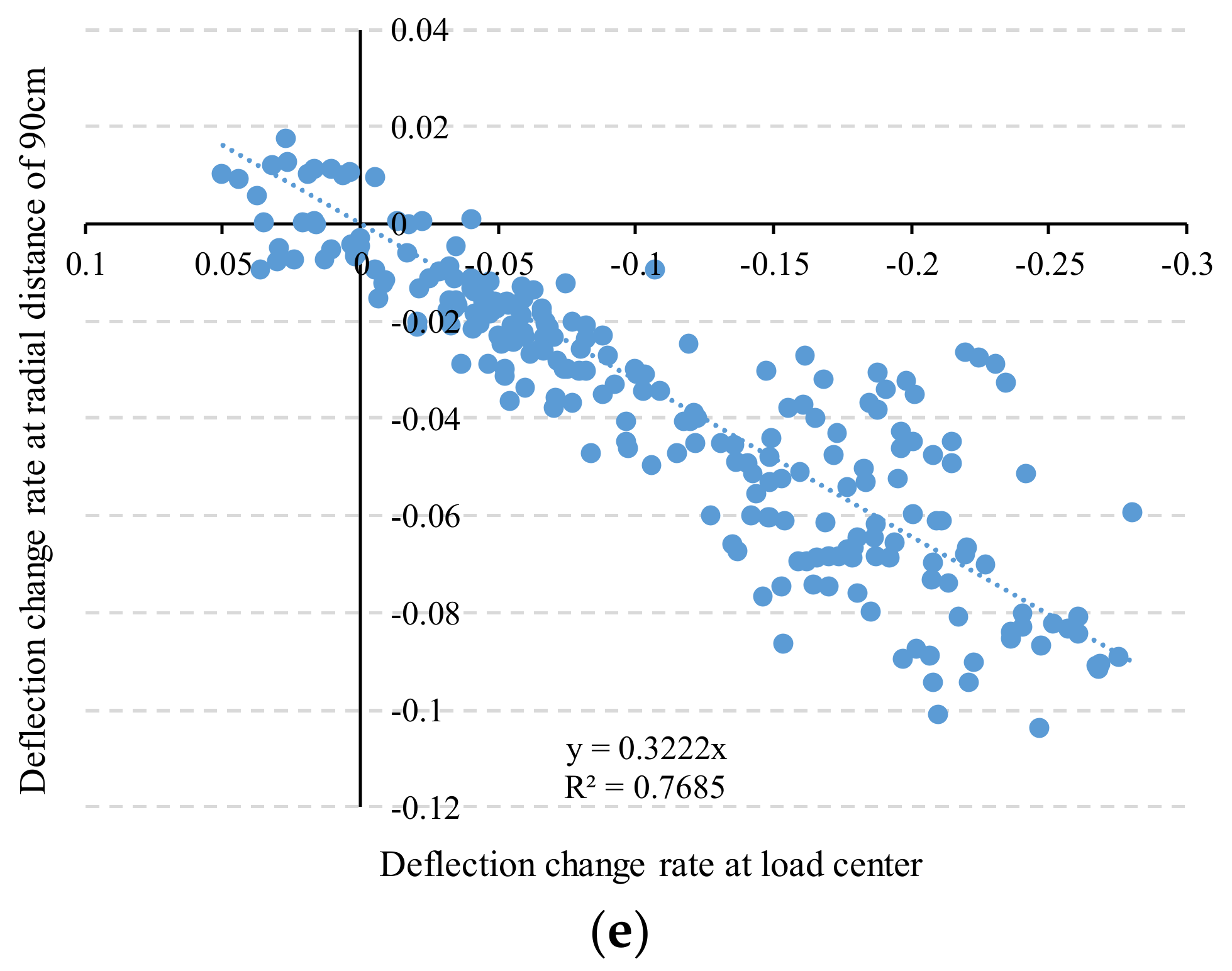
The plots of the deflection rate at the load center and each point at the radial distance from 20 to 90 cm were also analyzed, and the proportional function was used for fitting. The fitting results at different radial distances are shown in Figure 9. The ratio k and R2 of the deflection rate at each point and the load center are obtained, and the results are shown in Table 3.
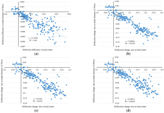
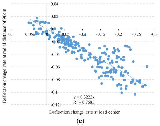
Figure 9.
Fitting results between deflection rate at different radial distances and load center deflection rates: (a) 20 cm; (b) 30 cm; (c) 45 cm; (d) 60 cm; (e) 90 cm.
Table 3.
Adjustment factors for deflection temperature.
From the fitting results, the fitting degree is better than that of the difference fitting in the previous section, and the results obtained are more accurate. Then, the deflection temperature correction model at different radial distances in the temperature-affected range is obtained, as shown in Equation (9). The meaning of each parameter is the same as above and will not be explained again.
5.2.3. Temperature Correction Based on the Deflection Change Rate at a Radial Distance of 20 cm
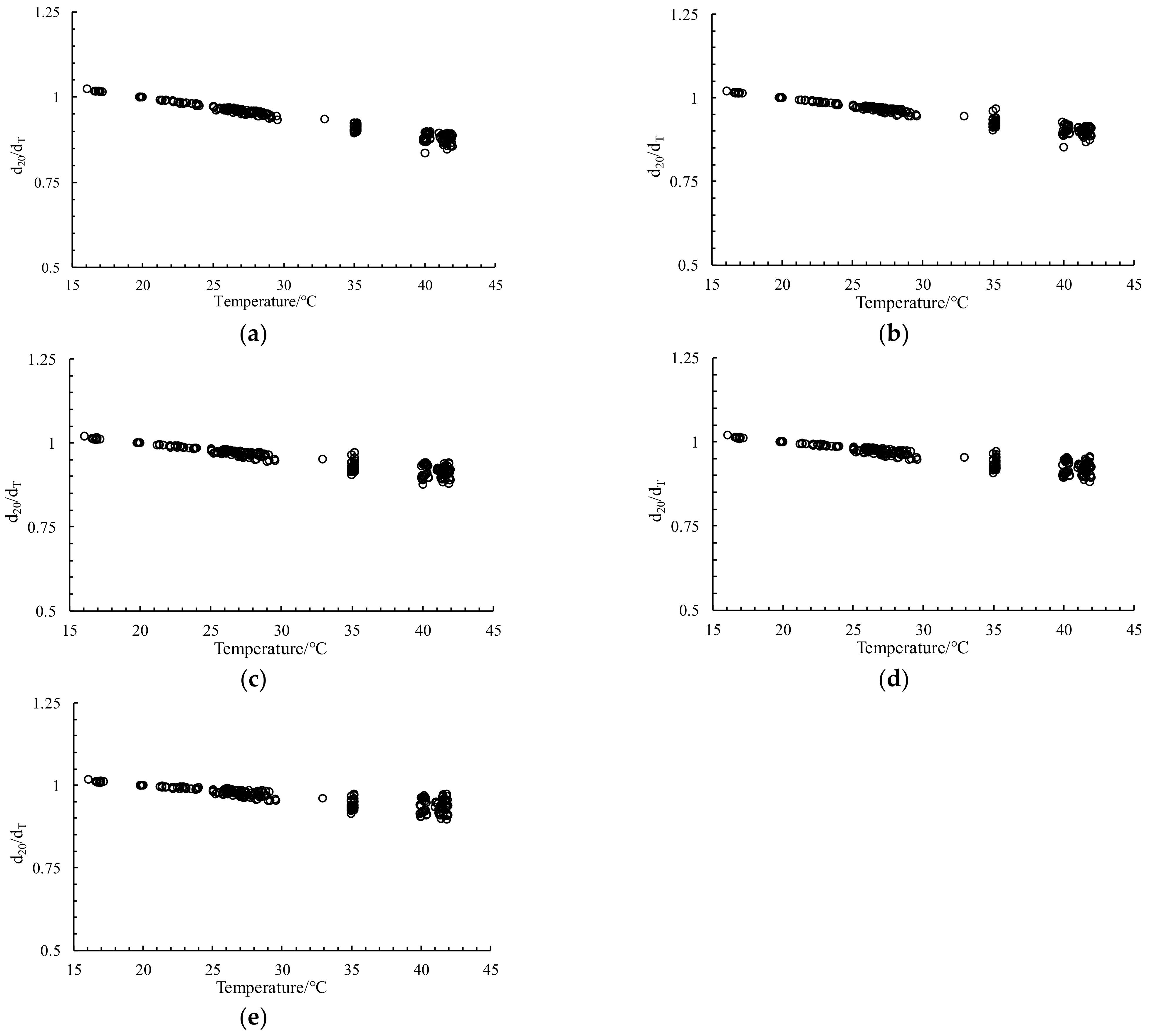
This method first selects a certain distance from 0 to 90 cm at each radial distance as the basis and then corrects other deflections in the deflection basin. The selection principle of this radial distance is that the fitting result between the deflection ratios before and after temperature correction and the temperature is the best. The temperature correction results for deflections at each radial distance were obtained by fitting the deflections from 0 to 90 cm to the temperature. The fitting result at the load center is shown in Figure 7, and the fitting results at other radial distances are shown in Figure 10.
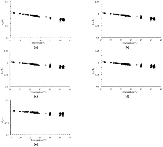
Figure 10.
Deflection fitting results at other radial distances: (a) 20 cm; (b) 30 cm; (c) 45 cm; (d) 60 cm; (e) 90 cm.
The correlation coefficients of the fitting results at each radial distance are shown in Table 4.
Table 4.
Fitting results at each radial distance.
As seen in the above table, the best fitting result was obtained for the point at a radial distance of 20 cm, with R2 reaching 0.964. Therefore, this method looks for the relationship between the change rate before and after the temperature correction of deflections at other radial distances and the deflection change rate at a radial distance of 20 cm to correct the deflection basin.
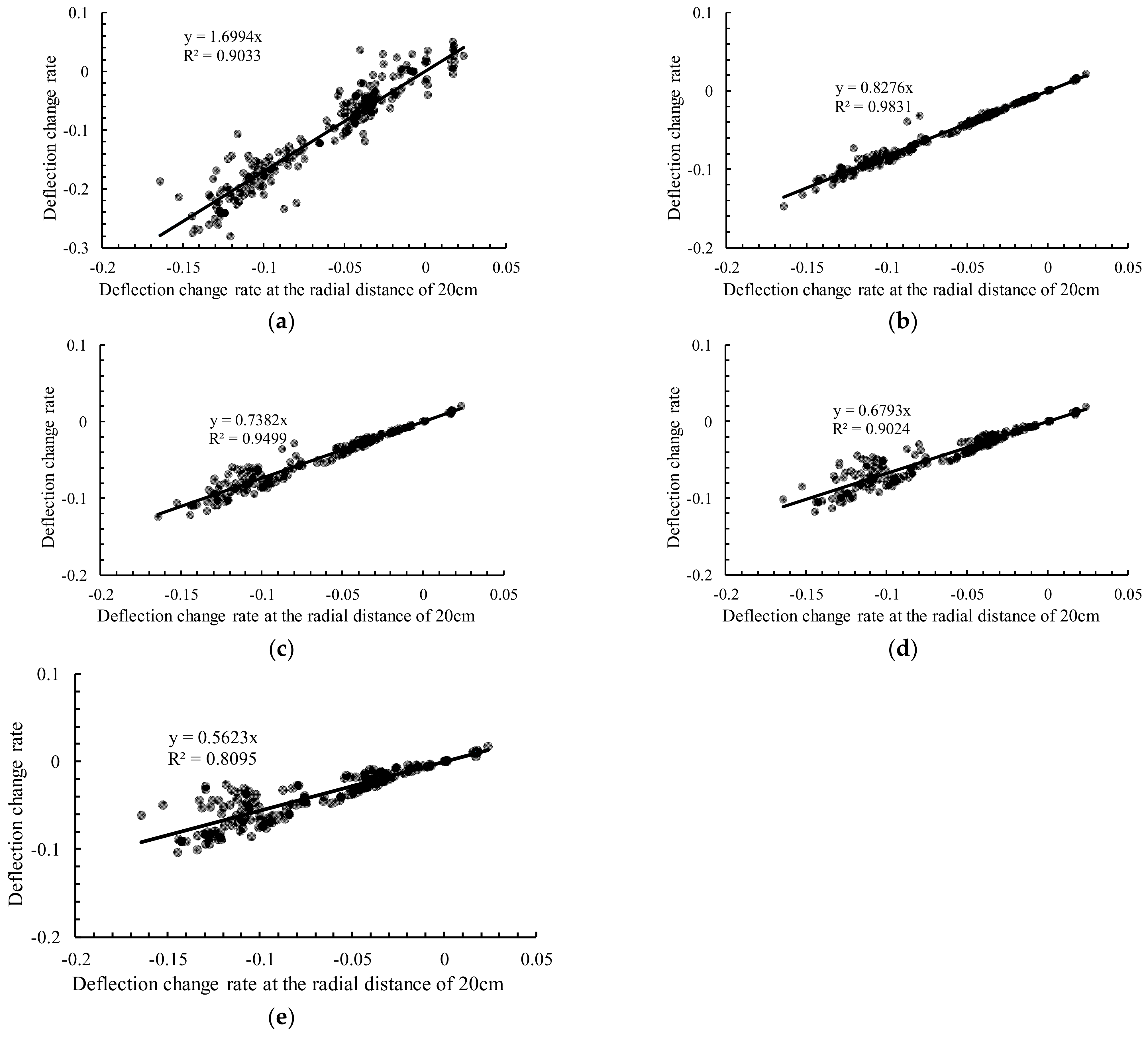
The deflection change rate at the load center and radial distance of 30~90 cm and the deflection change rate at the radial distance of 20 cm are fitted to obtain the ratio of the deflection change rate at each radial distance to the radial distance of 20 cm, and the results are shown in Figure 11. Adjustment coefficients for deflections are shown in Table 5.

Figure 11.
Deflection change ratio at each radial distance to the deflection change rate at 20 cm: (a) 20 cm; (b) 30 cm; (c) 45 cm; (d) 60 cm; (e) 90 cm.
Table 5.
Adjustment coefficients for deflections at each radial distance.
In the above graphs, the fitting degree of this method is better than that of the correction based on the load center deflection, and the obtained results are more accurate. The fitted images at radial distances from 30 to 90 cm are “comet” shaped, with the comet head at the (0, 0) coordinate and the comet tail at the third quadrant away from the (0, 0) point. The tail’s divergence becomes higher as the distance from the measurement point increases. In contrast, the fitted image at the load center is not “comet-like” and appears to be more diffuse.
According to St. Venant’s principle, this is due to the stress concentration at the load center. The load center is affected by the drop weight, and the configuration of the pavement has a great influence on the stress distribution generated by the drop weight, resulting in large fluctuations in the deflection at the load center due to the nearby stress distribution, while points farther away from the drop are hardly affected by this.
Then, a more suitable deflection temperature correction model at different radial distances in the temperature-affected range is obtained, as shown in Equation (10):
5.3. Validation
To validate the applicability and repeatability of the temperature correction model, measured deflection data from one other road section was used for comparative analysis. This pavement was made of 150 mm asphalt concrete (AC) and 450 mm fly ash with a three slag base. Platinum thermistor sensors were also embedded in the AC layer to collect the temperature data, as previously mentioned in the FWD test sections. Deflection measurement points are arranged in each lane at intervals of 30 m. The detailed deflection and temperature data are summarized in Table 6.
Table 6.
Measured deflection and temperature information.
The backcalculated layer moduli based on the deflection are shown in Table 7. Ea and Es are the backcalculated surface layer and subgrade moduli based on the uncorrected deflections, and EaT and EsT are the surface layer and subgrade moduli based on the corrected deflections using Equation (9).
Table 7.
The backcalculated layer moduli.
The definition of backcalculation accuracy is the proportion of the backcalculation moduli whose deviations are within an acceptable range. For the asphalt layer modulus, which has a variability of 15% in general, is considered acceptable when the surface layer backcalculation modulus is in the conventional deviation range of 85% to 115% [27]. Based on this, the percentage of EaT within the deviation range is 92.9%, while the percentage of Ea is 78.5%. The subgrade modulus is considered acceptable when it is within the deviation range of 90–110%. Similarly, the percentage of EsT within the deviation range was 92.9% while the percentage of Es was 85.7%.
The base modulus in this section has a high variability, and therefore no comparison is included. However, it can still be concluded from the comparison results of the surface layer and subgrade moduli that the accuracies of the backcalculation moduli based on the corrected deflection are more accurate. According to the above analysis, it is demonstrated that proposed deflection temperature model has good repeatability and applicability.
6. Conclusions
In this paper, the influence range of temperature on a deflection basin is studied through long-term FWD deflection detection on in-service highways, and a temperature correction formula for the deflection basin based on the deflection change rate is established. The conclusions are as follows:
- When performing the deflection temperature correction of an asphalt pavement in Shanghai, the temperature at the middle depth of the asphalt layer is more suitable for use as the representative temperature of the whole asphalt layer. In other regions, the location of the representative temperature may be different due to the different forms of pavement structures. Further validation analysis will be conducted later to clarify its applicability.
- The effective influence distance of temperature on the deflection basin is 90 cm. When the temperature correction of the deflection basin is performed, the deflection with a further radial distance can be uncorrected.
- We found that using the deflection change rate can obtain better deflection–temperature correction fitting results than the deflection difference. Then, we obtained a new model for deflection temperature correction based on the deflection change rate. On the basis of the new temperature correction model, we can evaluate the structural load-carrying capacity more precisely.
Author Contributions
Conceptualization, X.H. and L.S.; Methodology, X.H.; Software, Y.H.; Formal analysis, X.H. and Y.H.; Investigation, X.H. and J.L.; Data curation, J.L.; Writing—Original draft, X.H.; Writing—Review & editing, Y.H.; Visualization, X.H.; Funding acquisition, L.S. All authors have read and agreed to the published version of the manuscript.
Funding
This research was funded by the National Key R&D Program of China, grant number 2018YFB1600100.
Institutional Review Board Statement
Not applicable.
Informed Consent Statement
Not applicable.
Data Availability Statement
Not applicable.
Conflicts of Interest
The authors declare no conflict of interest.
References
- Oh, J.H.; Fernando, E.G.; Lee, S.I.; Holzschuher, C. Correlation of asphalt concrete layer moduli determined from laboratory and nondestructive field tests. J. Transp. Eng. 2012, 138, 361–370. [Google Scholar] [CrossRef]
- Li, C.; Ashlock, J.C.; Lin, S.; Vennapusa, P.K. In situ modulus reduction characteristics of stabilized pavement foundations by multichannel analysis of surface waves and falling weight deflectometer tests. Constr. Build. Mater. 2018, 188, 809–819. [Google Scholar] [CrossRef]
- Le, V.P.; Lee, H.J.; Flores, J.M.; Kim, W.J. New approach to construct master curve of damaged asphalt concrete based on falling weight deflectometer back-calculated moduli. J. Transp. Eng. 2016, 142, 04016048. [Google Scholar] [CrossRef]
- Wang, H.; Xie, P.; Ji, R.; Gagnon, J. Prediction of airfield pavement responses from surface deflections: Comparison between the traditional backcalculation approach and the ANN model. Road Mater. Pavement Des. 2021, 22, 1930–1945. [Google Scholar] [CrossRef]
- Chen, D.H.; Bilyeu, J.; Lin, H.H.; Murphy, M. Temperature correction on falling weight deflectometer measurements. Transp. Res. Rec. 2000, 1716, 30–39. [Google Scholar] [CrossRef]
- Pais, J.; Santos, C.; Pereira, P.; Kaloush, K. The adjustment of pavement deflections due to temperature variations. Int. J. Pavement Eng. 2020, 21, 1585–1594. [Google Scholar] [CrossRef]
- Shrp, K. SHRP Procedure for Temperature Correction of Maximum Deflections; Technical Report SHRP-P-654; PCS/Law Eng.: Washington, DC, USA, 1993. [Google Scholar]
- Li, M.; Wang, H. Development of ANN-GA program for backcalculation of pavement moduli under FWD testing with viscoelastic and nonlinear parameters. Int. J. Pavement Eng. 2019, 20, 490–498. [Google Scholar] [CrossRef]
- Minhoto, M.J.C.; Pais, J.C.; Pereira, P.A.; Picado-Santos, L.G. The influence of temperature variation in the prediction of the pavement overlay life. Road Mater. Pavement Des. 2005, 6, 365–384. [Google Scholar] [CrossRef]
- Schmalzer, P.N. Long-Term Pavement Performance Program Manual for Falling Weight Deflectometer Measurements; United States Federal Highway Administration, Office of Infrastructure Research and Development: New York, NY, USA, 2006.
- Fernando, E.G.; Liu, W.; Ryu, D. Development of a Procedure for Temperature Correction of Backcalculated AC Modulus; Texas Transportation Institute, Texas A & M University System: Bryan, TX, USA, 2001. [Google Scholar]
- Sousa, J.B.; Pais, J.C.; Saim, R.; Way, G.B.; Stubstad, R.N. Mechanistic-empirical overlay design method for reflective cracking. Transp. Res. Rec. 2002, 1809, 209–217. [Google Scholar] [CrossRef]
- Song, X.J.; Zeng, M.L.; Wang, L. A method of temperature correction for asphalt pavement dynamic deflection. J. Highw. Transp. Res. Dev. 2016, 33, 22–26. [Google Scholar] [CrossRef]
- Dong, Y.S. Research on the Dynamic Synthetic Deflection Correction Coefficient of Asphalt Pavement. Master’s Thesis, Chongqing Jiaotong University, Chongqing, China, 2010. [Google Scholar]
- Marshall, C.; Meier, R.; Welch, M. Seasonal temperature effects on flexible pavements in Tennessee. Transp. Res. Rec. J. Transp. Res. Board 2001, 1764, 89–96. [Google Scholar] [CrossRef]
- Baltzer, S.; Jansen, J.M. Temperature correction of asphalt-moduli for FWD-measurements. In Proceedings of the 4th International Conference, Bearing Capacity of Roads and Airfields, Minneapolis, MN, USA, 17–21 August 1994. [Google Scholar]
- Stubstad, R.N.; Baltzer, S.; Lukanen, E.O.; Ertman-Larsen, H.J. Prediction of AC mat temperatures for routine load/deflection measurements. In Proceedings of the 4th International Conference, Bearing Capacity of Roads and Airfields, Minneapolis, MN, USA, 17–21 August 1994. [Google Scholar]
- Noureldin, S.; Zhu, K.; Harris, D.; Li, S. Non-destructive estimation of pavement thickness, structural number and subgrade resilience along indot highways. Jt. Transp. Res. Program 2005, 158, 19–90. [Google Scholar]
- Larsen, H. Strategic Highway Research Program. Statens Vejlaboratorium Notat 1988. Available online: http://worldcat.org/issn/01095315 (accessed on 16 October 2022).
- Kim, Y.R.; Park, H. Use of Falling Weight Deflectometer Multi-Load Data for Pavement Strength Estimation; No. FHWA/NC/2002-006; U.S. Department of Transportation: Washington, DC, USA, 2002.
- Li, Y.; Li, J.; Hu, Y.; Li, S. Frequency adjustment method for in-situ seismic modulus of asphalt concrete. Int. J. Pavement Eng. 2022, 23, 2342–2350. [Google Scholar] [CrossRef]
- Park, D.Y.; Buch, N.; Chatti, K. Effective layer temperature prediction model and temperature correction via falling weight deflectometer deflections. Transp. Res. Rec. 2001, 1764, 97–111. [Google Scholar] [CrossRef]
- Transportation Officials. AASHTO Guide for Design of Pavement Structures; United States, The American Association of State Highway and Transportation Officials: Washington, DC, USA, 1993. [Google Scholar]
- Lukanen, E.O.; Stubstad, R.; Briggs, R.C.; Intertec, B. Temperature Predictions and Adjustment Factors for Asphalt Pavement; No. FHWA-RD-98-085; Turner-Fairbank Highway Research Center: McLean, VA, USA, 2000.
- Park, M.H.; Kim, Y.R.; Park, S. Temperature correction of multiload-level falling weight deflectometer deflections. Transp. Res. Rec. 2002, 1806, 3–8. [Google Scholar] [CrossRef]
- Zhu, J. Method of High-Precision Modulus Back-Calculation for Multi-Layer Structure of Asphalt Pavement. Ph.D. Thesis, Tongji University, Shanghai, China, 2013. [Google Scholar]
- Zang, G.S. Back-Calculation Method for Structural Parameters of Asphalt Pavement Based on Identity Points. Ph.D. Thesis, Tongji University, Shanghai, China, 2018. [Google Scholar]

Disclaimer/Publisher’s Note: The statements, opinions and data contained in all publications are solely those of the individual author(s) and contributor(s) and not of MDPI and/or the editor(s). MDPI and/or the editor(s) disclaim responsibility for any injury to people or property resulting from any ideas, methods, instructions or products referred to in the content. |
© 2022 by the authors. Licensee MDPI, Basel, Switzerland. This article is an open access article distributed under the terms and conditions of the Creative Commons Attribution (CC BY) license (https://creativecommons.org/licenses/by/4.0/).