Hybrid Adaptive Controller Design with Hysteresis Compensator for a Piezo-Actuated Stage

Abstract

Piezo-actuated stage (P-AS) has become the topic of considerable interest in the realm of micro/nanopositioning technology in the recent years owing to its advantages, such as high positioning accuracy, high response speed, and large output force. However, rate-dependent (RD) hysteresis, which is an inherent nonlinear property of piezoelectric materials, considerably restricts the application of P-AS. In this research paper, we develop a Hammerstein model to depict the RD hysteresis of P-AS. An improved differential evolution algorithm and a least-squares algorithm are used to identify the static hysteresis sub-model and the dynamic linear sub-model for the Hammerstein model, respectively. Then, a hysteresis compensator based on the inverse Bouc–Wen model is designed to compensate for the static hysteresis of the P-AS. However, the inevitable modeling error presents a hurdle to the hysteresis compensation. In addition, external factors, such as environmental noise and measurement errors, affect the control accuracy. To overcome these complications, a hybrid adaptive control approach based on the hysteresis compensator is adopted to increase the control accuracy. The closed-loop system stability is analyzed with the help of the Lyapunov stability theory. Finally, experimental results indicate that the raised control approach is effective for the accurate positioning of P-AS.

1. Introduction

Piezo-actuated stage (P-AS) driven by piezoelectric ceramics are broadly applied to projection lithography lenses, scanning probe microscopy, astronomical telescopes, modern optics, other advanced optoelectronic devices, and ultraprecision systems [1,2,3] owing to high resolutions and response speeds and the impregnability of the magnetic fields [4,5]. However, the intrinsic rate-dependent (RD) hysteresis of piezoelectric ceramic materials significantly affects the control and positioning accuracies of P-AS [6,7,8]. The response of RD hysteresis characteristic exhibits a special multi-value mapping relationship, where the P-AS output depends on the current input and the previous output of P-AS [9]. In addition, the RD characteristic indicates that the frequency of the P-AS input is one of the important factors affecting their output [10]. Therefore, current research focuses on developing reasonable control strategies to depress the hysteresis characteristic of the P-AS [11,12,13].

At present, the methods for eliminating hysteresis are mainly divided into two categories: feedforward compensation control methods based on the hysteretic inverse model and feedback control methods. The feedforward compensation control method needs to establish the hysteretic model first, then obtain the inverse model of the system via resolution or identification of the hysteretic model, and finally construct the feedforward controller based on the inverse model [14,15]. Common models for characterizing hysteresis include the Duhem model [16], backlash-like model [17], Bouc–Wen (BW) model [18,19,20], Preisach model [21,22], Prandtl–Ishlinskii model [23,24,25], and Krasnoselskii–Pokrovskii model [26,27,28]. In addition, there are various other models in the literature to depict the complex hysteresis of piezoelectric motors [29,30,31]. The feedforward compensation control method proposed in the above literature can effectively suppress the effect of hysteresis on system accuracy and achieve accurate tracking control. However, the accuracy of modeling seriously affects the performance of feedforward compensation control methods. The control effect of feedforward controllers is significantly weakened if modeling errors and uncertain noise exist. In addition, the feedforward controller has poor robustness to resist the interference of external disturbances.

To overcome the shortcomings of feedforward compensation control methods, feedback control methods have been proposed [32,33,34]. The common feedback control methods include PID control [35], sliding mode control [36,37], iterative learning control [38,39], adaptive control [40], robust control [41,42], model predictive control [43,44], and modified repetitive control [45]. These control methods can suppress external disturbances and increase the control accuracy compared with the feedforward compensation control methods [46].

Adaptive control is a feedback control method that can compensate for the modeling error and external uncertain noise of the feedforward compensation control methods [47,48,49]. Exploiting this property, we propose a hybrid adaptive control (HAC) strategy based on a hysteresis controller to decrease the influence of the hysteresis characteristic for P-AS and realize precise positioning. First, a Hammerstein model is proposed consisting of a BW hysteresis sub-model and dynamic linear sub-model to depict the RD hysteresis characteristic for P-AS. An improved differential evolution algorithm and a least-squares algorithm are employed to identify the two sub-models, respectively. Then, the inverse BW model is identified by the improved differential evolution algorithm as a compensator to handle the RD hysteresis characteristic of P-AS. To reduce the effects of modeling errors and uncertain noise, a hybrid adaptive controller is proposed, and the stability of the raised approach is certified by the Lyapunov theory. The effectiveness of the adopted approach is demonstrated by a series of experiments involving comparisons with the hysteresis compensation controller based on the inverse BW model and the model reference adaptive controller (MRAC). The main contribution of this research is the raised HAC method for the precise positioning of P-AS.

The remainder of this work is organized as follows. The Hammerstein model for P-AS is presented in Section 2. The design program of a hybrid adaptive controller based on the hysteresis compensator and the stability proof are presented in Section 3. Experimental results confirming the efficiency of the raised control strategy are given in Section 4. Conclusions are presented in Section 5.

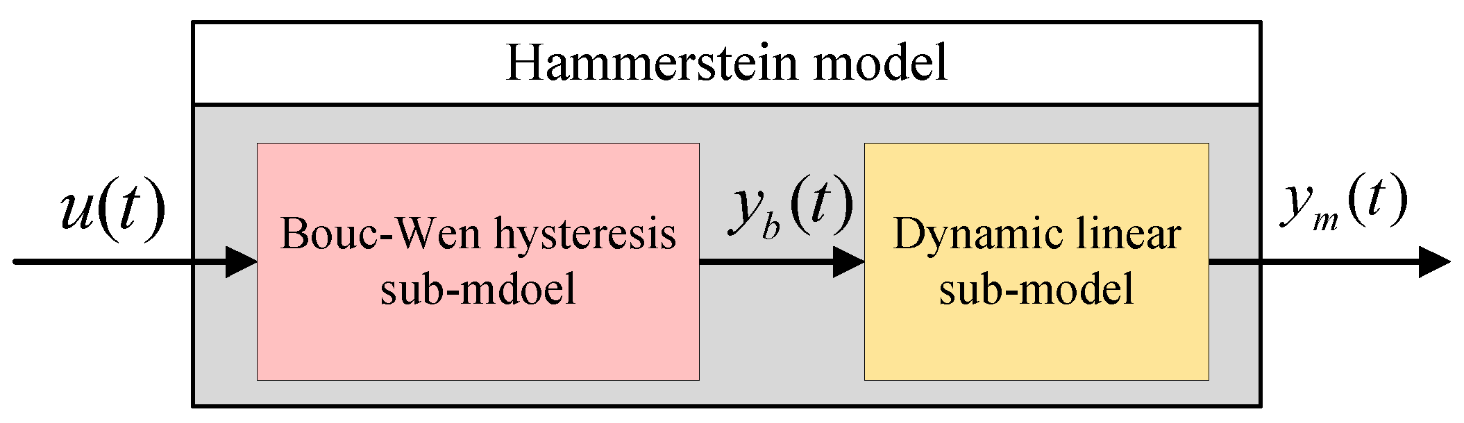
2. Hysteresis Modeling

To depict the RD hysteresis characteristic of P-AS, a Hammerstein model consisting of a BW hysteresis sub-model and a dynamic linear sub-model is established. A schematic diagram of the Hammerstein model is shown in Figure 1. Then, the identification algorithms of these sub-models are introduced.

2.1. BW Hysteresis Sub-Model Identification Based on Improved Differential Evolution Algorithm

A generalized BW model that can describe hysteresis as differential equations was suggested by Bouc and Wen. In this study, the BW model is used as the hysteresis sub-model to describe the static hysteresis of the P-AS, and its expression is shown as follows:

$$\left\{\begin{array}{c}{y}_b\left(t\right)=dV\left(t\right)-H\left(t\right)\hfill \\ \dot{H}\left(t\right)=a\dot{V}\left(t\right)-b|\dot{V}\left(t\right)|H\left(t\right)-c\dot{V}\left(t\right)\left|H\left(t\right)\right|\hfill \end{array}\right.$$

(1)

where $V\left(t\right)$ and $y_b\left(t\right)$ represent the input and output of the BW model, respectively, at time t. $H\left(t\right)$ and d denote the hysteresis term and actuator factor, respectively. a, b, and c are the identified parameters of the BW hysteresis sub-model, which determine the amplitude and shape of the BW model. Because of the complexity of the BW hysteresis sub-model, the conventional algorithms are not suitable for identifying unknown parameters. The differential evolution algorithm is an intelligent optimization algorithm that is commonly used in system identification owing to its simple structure and fast convergence. However, the differential evolution algorithm easily falls into local minima. Therefore, an improved differential evolution algorithm is proposed to enhance its global search capability; the evolution of two populations is used, and the algorithm shares the optimum individual resources by information exchange. In this study, the parameters of the BW hysteresis sub-model are obtained by the improved differential evolution algorithm. Equation (1) is rewritten as follows:

$$y_b\left(t\right)=F(t,V\left(t\right),H\left(t\right),\mathrm{\Theta })$$

(2)

where $\mathrm{\Theta }=[d,a,b,c]$ is the vector of unknown parameters to be identified. The pseudo-code of the improved differential evolution algorithm is presented in Algorithm 1.

Algorithm 1 Improved differential evolution algorithm for obtaining the parameters of the BW hysteresis sub-model.

Input:  Define the current iteration of this algorithm as N, where $N\le N_{max}$. The dimension of parameters that need to be obtained is $N_{\theta }$. The number of iterations for the two populations before the exchange of information is $K_{\theta }$. The range of the unknown-parameter vector is $\left[{\mathrm{\Theta }}_{min},{\mathrm{\Theta }}_{max}\right]$. Define $D_{\theta }$ as the dimension of the population. ${\theta }_i^j\left(n\right)$ represents the i-th individual of the j-th population in the n-th generation, where $i=1,2,\dots ,D_{\theta }$; $j=1,2$; and $n=1,2,\dots ,N_{\theta }$. Define P as the probability of crossover and mutation for the second population. Output:  The optimal-parameter vector is ${\mathrm{\Theta }}^{*}$. 1: Initialize ${\mathrm{\Theta }}^j\left(0\right)={\mathrm{\Theta }}_{min}^j+rand(D_{\theta },N_{\theta })\left({\mathrm{\Theta }}_{max}-{\mathrm{\Theta }}_{min}\right)$, where $(D_{\theta },N_{\theta })$ is a matrix with random element values ranging from 0 to 1. 2: Define a fitness function $F_{\theta }\left({\theta }_i^j\left(n\right)\right)=\frac{1}{2}{\sum }_{t=1}^T\left[y\left(t\right)-y_b\left(t\right)\right]$, where $y\left(t\right)$ represents the output of the P-AS at time t, and T represents the size of sample. Define $F_j^{*}$ and ${\mathrm{\Theta }}_j^{*}$ as the optimal value of the fitness function and j-th optimal-parameter vector, respectively. 3: Update the two populations. Define ${\alpha }^j$ as the variation factor of the two populations, $\beta$ as the crossover probability, and a random number $l_i^j\in [0,1]$. $p_i^j(n+1)={\theta }_{i_1}^j\left(n\right)+{\alpha }^j\left({\theta }_{i_2}^j\left(n\right)-{\theta }_{i_3}^j\left(n\right)\right)$ for $i\ne i_1\ne i_2\ne i_3$. $q_i^j(n+1)=p_i^j(n+1)$ if $l_i^j\le \beta$, and $q_i^j(n+1)={\theta }_i^j\left(n\right)$ if $l_i^j>\beta$. ${\theta }_i^j(n+1)=q_i^j(n+1)$ if $F_{\theta }\left(q_i^j\left(n\right)\right)\le F_{\theta }\left({\theta }_i^j\left(n\right)\right)$, and ${\theta }_i^j(n+1)={\theta }_i^j(n+1)$ if $F_{\theta }\left(q_i^j\left(n\right)\right)>F_{\theta }\left({\theta }_i^j\left(n\right)\right)$. Compute the objective function and identify the population whose objective function is smaller. 4: For the first population, return to the third step until the $K_{\theta }$-th iteration is reached. 5: For the second population, if $P<0.5$, execute the crossover operator; otherwise, execute the mutation operation. Then, repeat the third step until the $K_{\theta }$-th iteration is reached. 6: The global best fitness $F^{*}$ and the global best individual ${\mathrm{\Theta }}^{*}$ are calculated as follows $F^{*}=min(F^1,F^2)$ ${\mathrm{\Theta }}^{*}={\mathrm{\Theta }}^j$, where j meets $F^j=F^{*}$. 7: Set $N=N+1$ and repeat the third step. If $N>N_{max}$, return ${\mathrm{\Theta }}^{*}$.

A sinusoidal input signal expressed as $y\left(t\right)=18sin(2\pi t-0.5\pi t)+18$ was adopted to identify the parameters of the BW model for the P-AS. The results for the identification via the proposed algorithm were $d=1.099$, $a=-0.5257$, $b=1.019$, and $c=-0.208$.

2.2. Dynamic Linear Sub-Model Identification Based on Least-Squares Algorithm

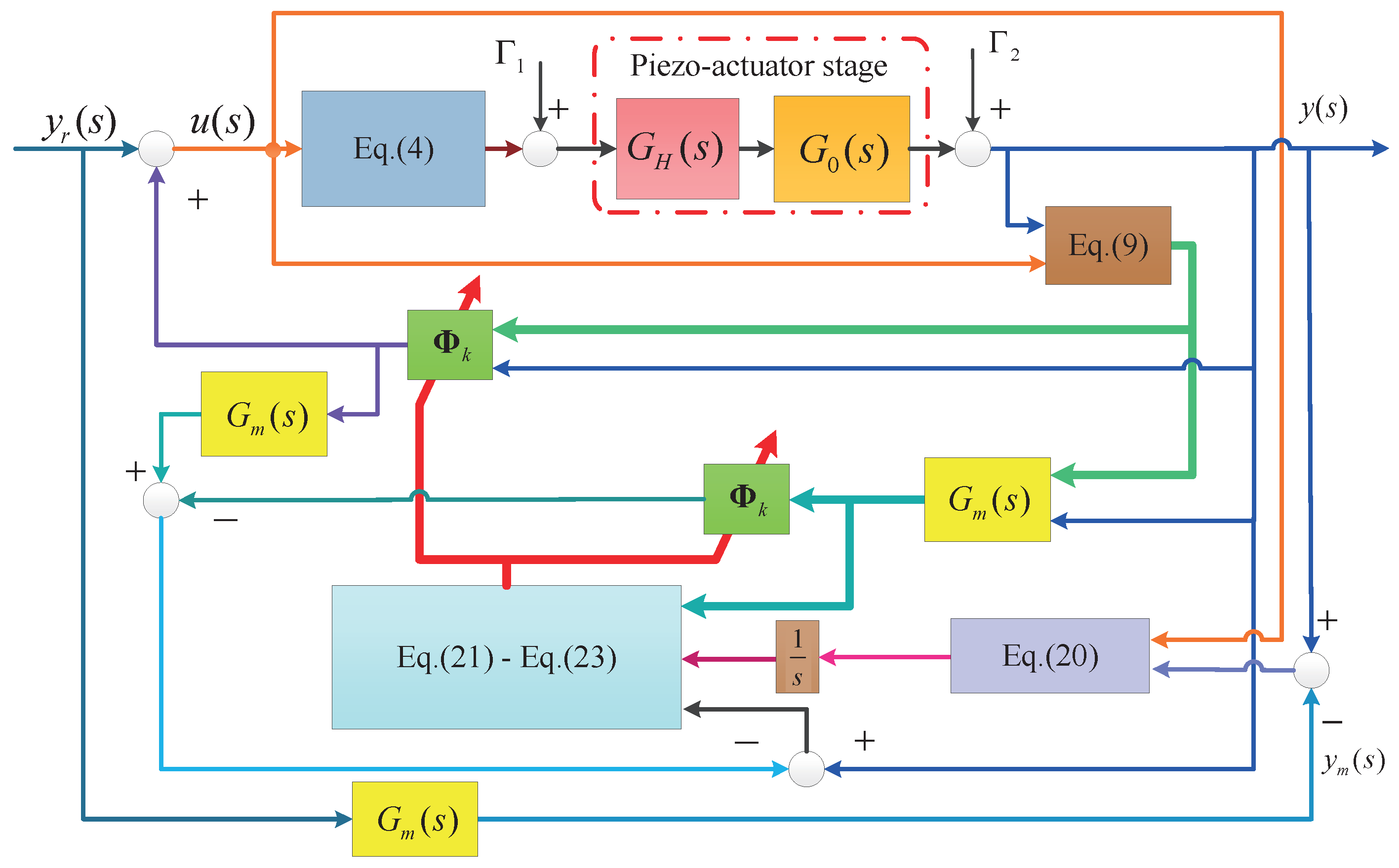
To develop an RD hysteresis dynamic linear sub-model that can characterize the P-AS, a sinusoidal swept signal with the frequency of 1–100 Hz is adopted to drive the P-AS. A least-squares algorithm is employed to obtain the dynamic linear sub-model using the MATLAB system identification toolbox, as described in [18]. The dynamic linear sub-model is expressed as follows:

$$G_m\left(s\right)=\frac{1.58\ast {10}^{4}s+10}{{10}^{-3}{s}^3+3.2s^2+1.58\ast {10}^{4}s+10}$$

(3)

3. HAC Design

3.1. Inverse BW Model-Based Hysteresis Compensator Design

To compensate for the RD hysteresis characteristic of P-AS, the inverse compensator is designed by solving the inverse BW model according to (1) as follows:

$$\left\{\begin{array}{c}V\left(t\right)=d^{\prime }\left(y_r\left(t\right)+H_I\left(t\right)\right)\hfill \\ {\dot{H}}_I\left(t\right)=a^{\prime }{\dot{y}}_r\left(t\right)-b^{\prime }\left|{\dot{y}}_r\left(t\right)\right|H_I\left(t\right)-c^{\prime }{\dot{y}}_r\left(t\right)\left|H_I\left(t\right)\right|\hfill \end{array}\right.$$

(4)

where $V\left(t\right)$ represents the output voltage of the hysteresis compensator, $d^{\prime }$ is the actuator factor, and $y_r\left(t\right)$ represents the expected displacement. $d^{\prime }=1.105$, $a^{\prime }=-0.445$, $b^{\prime }=1.081$, and $c^{\prime }=-0.153$ were identified by the improved differential evolution algorithm.

3.2. HAC Design Based on Hysteresis Compensator

The open-loop control system based on the hysteresis compensator for P-AS in the complex field is expressed as follows:

$$y\left(s\right)=\left[u\left(s\right){G_H}^{-1}+{\mathrm{\Gamma }}_1\right]G_H{G}_0\left(s\right)+{\mathrm{\Gamma }}_2$$

(5)

where $u\left(s\right)$ and $y\left(s\right)$ represent the input and output of the open-loop control, respectively, and $G_H$ and $G_0$ represent the hysteresis sub-model and linear sub-model of the P-AS, respectively. ${G_H}^{-1}$ is the transfer function for the inverse compensator. ${\mathrm{\Gamma }}_1$ and ${\mathrm{\Gamma }}_2$ represent the input and measurement noise of the P-AS, respectively. Then, the transfer function of the open-loop control can be denoted as follows:

$$G\left(s\right)=\frac{y\left(s\right)}{u\left(s\right)}=\left[{G_H}^{-1}+\frac{{\mathrm{\Gamma }}_1}{u\left(s\right)}\right]G_H{G}_0\left(s\right)+\frac{{\mathrm{\Gamma }}_2}{u\left(s\right)}$$

(6)

Define $k_b{f}_1=\left({\mathrm{\Gamma }}_1{G}_H\right)/u\left(s\right)$ and $k_b{f}_2={\mathrm{\Gamma }}_2/u\left(s\right)$. Then, (6) can be rewritten as:

$$G\left(s\right)=G_0\left(s\right)\left[1+k_b{f}_1\left(s\right)\right]+k_b{f}_2\left(s\right)$$

(7)

where $f_1\left(s\right)$ and $f_2\left(s\right)$ represent the input and output unmodeled dynamics, respectively, of the P-AS. The scalar parameter $k_b>0$ represents the rate of the unmodeled dynamic. To achieve precise tracking control, a hybrid adaptive controller is designed in this section. First, we exploit two accessorial vectors ${\omega }_1\left(s\right)$ and ${\omega }_2\left(s\right)$ and define:

$$\left\{\begin{array}{c}{\dot{\omega }}_1\left(s\right)={\mathbf{A}}_1{\omega }_1\left(s\right)+{\mathbf{B}}_{1}u\left(s\right)\hfill \\ {\dot{\omega }}_2\left(s\right)={\mathbf{A}}_2{\omega }_2\left(s\right)+{\mathbf{B}}_{2}y\left(s\right)\hfill \end{array}\right.$$

(8)

where ${\mathbf{A}}_{\mathbf{1}}$ and ${\mathbf{A}}_{\mathbf{2}}$ are two-dimensional matrices, and ${\mathbf{B}}_{\mathbf{1}}$ and ${\mathbf{B}}_{\mathbf{2}}$ are two-dimensional column vectors. The solution of (8) is as follows:

$$\left\{\begin{array}{c}{\omega }_1\left(s\right)={\left(s\mathbf{I}-{\mathbf{A}}_1\right)}^{-1}{\mathbf{B}}_{1}u\left(s\right)\hfill \\ {\omega }_2\left(s\right)={\left(s\mathbf{I}-{\mathbf{A}}_2\right)}^{-1}{\mathbf{B}}_{2}y\left(s\right)\hfill \end{array}\right.$$

(9)

In accordance with (9), the control law is designed as follows:

$$\begin{array}{cc}\hfill u\left(s\right)& =\left[\begin{array}{ccc}{\mathbf{\Phi }}_{1k}^{\mathrm{T}}& {\mathbf{\Phi }}_{2k}^{\mathrm{T}}& {\Phi }_{3k}\end{array}\right]\left[\begin{array}{c}{\omega }_{\mathbf{1}}\left(s\right)\\ {\omega }_{\mathbf{2}}\left(s\right)\\ y\left(s\right)\end{array}\right]+y_r\left(s\right)\hfill \\ \hfill & ={\mathbf{\Phi }}_{1k}^{\mathrm{T}}{\omega }_1\left(s\right)+{\mathbf{\Phi }}_{2k}^{\mathrm{T}}{\omega }_2\left(s\right)+{\Phi }_{3k}y\left(s\right)+y_r\left(s\right)\hfill \end{array}$$

(10)

where ${\mathbf{\Phi }}_k^{\mathrm{T}}=\left[{\mathbf{\Phi }}_{1k}^{\mathrm{T}},{\mathbf{\Phi }}_{2k}^{\mathrm{T}},{\Phi }_{3k}\right]$ is the parameter vector of the hybrid adaptive controller, which is a constant vector at time $[t_k,t_{k+1})$. It is adjusted at time $t_{k+1}$ for $k=0,1,2,\dots ,K$. K represents the maximum sampling for the control system.

Theorem 1. 

Define $G_0\left(s\right)$ as the reference model of the P-AS control system based on the compensator. Because $k_b=0$, we have ${\mathbf{\Phi }}_k\equiv {\mathbf{\Phi }}^{*}$ to equate the transfer function $G\left(s\right)$ of P-AS control system based on the hybrid adaptive controller to $G_0\left(s\right)$, where ${\mathbf{\Phi }}_k=\left[{\mathbf{\Phi }}_{1k}^{\mathrm{T}},{\mathbf{\Phi }}_{2k}^{\mathrm{T}},{\Phi }_{3k}\right]$, ${\mathbf{\Phi }}^{*}$ is a constant vector.

$$G_0\left(s\right)=\frac{y_m\left(s\right)}{y_r\left(s\right)}=G\left(s\right)=\frac{y\left(s\right)}{u\left(s\right)}·\frac{u\left(s\right)}{y_r\left(s\right)}$$

(11)

Proof. 

By substituting (9) into (10), the control law is obtained:

$$u\left(s\right)={\mathbf{\Phi }}_{1k}^{\mathrm{T}}{(s\mathbf{I}-{\mathbf{A}}_1)}^{-1}{\mathbf{B}}_{1}u\left(s\right)+{\mathbf{\Phi }}_{2k}^{\mathrm{T}}{(s\mathbf{I}-{\mathbf{A}}_2)}^{-1}{\mathbf{B}}_{2}y\left(s\right)+{\Phi }_{3k}y\left(s\right)+y_r\left(s\right)$$

(12)

Because $k_b=0$ according to (7), the output of the control system is $y\left(s\right)=G_m\left(s\right)u\left(s\right)$. Then, (12) can be denoted as follows:

$$u\left(s\right)={[1-{\mathbf{\Phi }}_1^{*\mathrm{T}}{(s\mathbf{I}-{\mathbf{A}}_1)}^{-1}{\mathbf{B}}_1-{\mathbf{\Phi }}_2^{*\mathrm{T}}{(s\mathbf{I}-{\mathbf{A}}_2)}^{-1}{\mathbf{B}}_2{G}_0\left(s\right)-{\Phi }_3^{*}{G}_0\left(s\right)]}^{-1}{y}_r\left(s\right)$$

(13)

According to (13), (11) becomes:

$$G_m\left(s\right)=\frac{G_0\left(s\right)}{1-{\mathbf{\Phi }}_1^{*\mathrm{T}}{(s\mathbf{I}-{\mathbf{A}}_1)}^{-1}{\mathbf{B}}_1-{\mathbf{\Phi }}_2^{*\mathrm{T}}{(s\mathbf{I}-{\mathbf{A}}_2)}^{-1}{\mathbf{B}}_2{G}_0\left(s\right)-{\Phi }_3^{*}{G}_0\left(s\right)}$$

(14)

Then, by substituting (13) and (14) into (12), we have:

$$y\left(s\right)=G_m\left(s\right)[{({\mathbf{\Phi }}_k-{\mathbf{\Phi }}^{*})}^{\mathrm{T}}\omega \left(s\right)+y_r\left(s\right)]+k^{*}f\left(s\right)u\left(s\right)$$

(15)

where

$$\begin{array}{cc}\hfill f\left(s\right)=& f_1\left(s\right)-G_m\left(s\right)[{\Phi }_3^{*}+{\mathbf{\Phi }}_2^{*\mathrm{T}}{(sI-A)}^{-1}B]G_0\left(s\right)f_2\left(s\right)\hfill \\ \hfill & +G_m\left(s\right)f_2\left(s\right)[1-{\mathbf{\Phi }}_1^{*\mathrm{T}}{(sI-A)}^{-1}B]\hfill \end{array}$$

(16)

We define $e_1\left(s\right)=y\left(s\right)-y_m\left(s\right)$ as the error between output values of P-AS and the reference model. By combining (7), (10), and (14), we obtain:

$$e_1\left(s\right)=G_m\left(s\right){({\mathbf{\Phi }}_k-{\mathbf{\Phi }}^{*})}^{\mathrm{T}}\omega \left(s\right)+k_b^{*}fu\left(s\right)$$

(17)

Because $k_b^{*}=0$, it has ${\mathbf{\Phi }}_k\equiv {\mathbf{\Phi }}^{*}$, so that the error $e_1\left(s\right)=0$.

This completes the proof. □

Next, the adaptive law is adopted to modulate ${\mathbf{\Phi }}_k$ online. To facilitate the calculation of the adaptive law, (17) is rewritten via inverse Laplace transformation:

$$y_f\left(t\right)=-{({\mathbf{\Phi }}_k-{\mathbf{\Phi }}^{*})}^{\mathrm{T}}{G}_m\left(t\right)\omega \left(t\right)+G_m\left(t\right){({\mathbf{\Phi }}_k-{\mathbf{\Phi }}^{*})}^{\mathrm{T}}\omega \left(t\right)$$

(18)

where $y_f\left(t\right)$ is an instrumental variable. We define $\xi \left(t\right)=G_m\left(t\right)\omega \left(t\right)$ and $\eta \left(t\right)=f\left(t\right)u\left(t\right)$, where $\omega {\left(t\right)}^{\mathrm{T}}=[{\omega }_1\left(t\right),{\omega }_2\left(t\right),y\left(t\right)]$. Next, the augmented error is obtained as follows:

$$\begin{array}{cc}\hfill {\epsilon }_1\left(t\right)& =e_1\left(t\right)-y_f\left(t\right)\hfill \\ \hfill & ={({\mathbf{\Phi }}_k-{\mathbf{\Phi }}^{*})}^{\mathrm{T}}\xi \left(t\right)+k_b^{*}\eta \left(t\right)\hfill \end{array}$$

(19)

We define $\epsilon \left(t\right)={\epsilon }_1\left(t\right)/m\left(t\right)$ and $\psi \left(t\right)=\xi \left(t\right)/m\left(t\right)$, where $m\left(t\right)$ satisfies the differential equation as follows:

$$\begin{array}{c}\hfill \dot{m}\left(t\right)=-{\delta }_{0}m\left(t\right)+{\delta }_1\mathbf{E}{\mathbf{R}}^T\left(t\right)\end{array}$$

(20)

Here, $\mathbf{E}$ is a three-dimensional identity matrix. Both ${\delta }_0$ and ${\delta }_1$ are positive real numbers, and $\mathbf{R}\left(t\right)={[\left|u\left(t\right)\right|,\left|y\left(t\right)\right|,1]}^T$. $m\left(0\right)$ is the default value of $m\left(t\right)$, which satisfies $m\left(0\right)>{\delta }_0/{\delta }_1$. According to (20), $\epsilon \left(t\right)$ can be rewritten as:

$$\begin{array}{c}\hfill \epsilon \left(t\right)={({\mathbf{\Phi }}_k-{\mathbf{\Phi }}^{*})}^{\mathrm{T}}\psi \left(t\right)+k_b^{*}\eta \left(t\right)/m\left(t\right)\end{array}$$

(21)

To adjust ${\mathbf{\Phi }}_k$ online, the adaptive law is designed as:

$$\begin{array}{c}\hfill {\mathbf{\Phi }}_{k+1}={\mathbf{\Phi }}_k-\frac{1}{T_k}{\int }_{t_k}^{t_{k+1}}\frac{\sigma \left(t\right)\epsilon \left(t\right)\psi \left(t\right)}{1+{\psi }^T\left(t\right)\psi \left(t\right)}dt\end{array}$$

(22)

where $T_k=t_{k+1}-t_k$. $\sigma \left(t\right)$ is defined as:

$$\sigma \left(t\right)=\left\{\begin{array}{c}0,\left|\epsilon \left(t\right)\right|\le v_0\hfill \\ 1,\left|\epsilon \left(t\right)\right|>v_0\hfill \end{array}\right.$$

(23)

where $v_0$ is a positive constant that satisfies:

$$2k^{*}\left|\eta \left(t\right)\right|/m\left(t\right)\le v_0\le k^{*}{\rho }_0,{\rho }_0>0$$

(24)

Then, we can obtain the control law of HAC. A schematic of the HAC design based on the hysteresis compensator is shown in Figure 2.

3.3. Stability Analysis of System

We define the Lyapunov function as follows:

$$V_k=\frac{1}{2}{{\theta }_k}^{\mathrm{T}}{\theta }_k$$

(25)

where ${\theta }_k=({\mathbf{\Phi }}_k-{\mathbf{\Phi }}^{*})$. The derivation of (25) is as follows:

$$\begin{array}{cc}\hfill \mathrm{\Delta }{V}_k& =V_{k+1}˘V_k\hfill \\ \hfill & =\frac{1}{2}{\theta }_{k+1}^T{\theta }_{k+1}-\frac{1}{2}{\theta }_k^T{\theta }_k\hfill \\ \hfill & ={\left[\frac{1}{2}{\theta }_{k+1}+\frac{1}{2}{\theta }_k\right]}^T\left[{\theta }_{k+1}˘{\theta }_k\right]\hfill \\ \hfill & ={\left[\frac{1}{2}{\theta }_{k+1}˘{\theta }_k+\frac{1}{2}{\theta }_k+{\theta }_k\right]}^T[{\theta }_{k+1}˘{\theta }_k]\hfill \end{array}$$

(26)

We define $\mathrm{\Delta }{\theta }_k={\theta }_{k+1}-{\theta }_k$. Using (22), $\mathrm{\Delta }{\theta }_k$ can be rewritten as:

$$\begin{array}{cc}\hfill \mathrm{\Delta }{\theta }_k& ={\theta }_{k+1}-{\theta }_k\hfill \\ \hfill & =({\mathbf{\Phi }}_{k+1}-{\mathbf{\Phi }}_k)\hfill \\ \hfill & =-\frac{1}{T_k}{\int }_{t_k}^{t_{k+1}}\frac{\sigma \left(t\right)\epsilon \left(t\right)\psi \left(t\right)}{1+{\psi }^T\left(t\right)\psi \left(t\right)}dt\hfill \end{array}$$

(27)

By substituting (21) and (28) into (26), we obtain:

$$\begin{array}{cc}\hfill \mathrm{\Delta }{V}_k=& -\frac{1}{2}\left[-\frac{1}{T_k}{\int }_{t_k}^{t_{k+1}}\frac{\sigma [{\theta }_k^T\psi \left(t\right)+k_b^{*}\eta \left(t\right)/m\left(t\right)]\psi \left(t\right)}{1+{\psi }^T\left(t\right)\psi \left(t\right)}dt+2{\theta }_k^T\right]·\hfill \\ \hfill & \left[\frac{1}{T_k}{\int }_{t_k}^{t_{k+1}}\frac{\sigma [{\theta }_k^T\psi \left(t\right)+k_b^{*}\eta \left(t\right)/m\left(t\right)]\psi \left(t\right)}{1+{\psi }^T\left(t\right)\psi \left(t\right)}dt\right]\hfill \end{array}$$

(28)

We define ${\mathsf{\eta }}^{*}\left(t\right)=\eta \left(t\right){{\theta }_k^T}^{-1}$. $\mathrm{\Delta }{V}_k$ can be rewritten as:

$$\begin{array}{cc}\hfill \mathrm{\Delta }{V}_k& =-\frac{1}{2}\left[-\frac{1}{T_k}{\int }_{t_k}^{t_{k+1}}\frac{\sigma [\psi \left(t\right)+k_b^{*}{\eta }^{*}\left(t\right)/m\left(t\right)]\psi \left(t\right)}{1+{\psi }^T\left(t\right)\psi \left(t\right)}dt+2{\theta }_k^T\right]·\hfill \\ \hfill & \left[\frac{1}{T_k}{\int }_{t_k}^{t_{k+1}}\frac{\sigma [\psi \left(t\right)+k_b^{*}{\eta }^{*}\left(t\right)/m\left(t\right)]\psi \left(t\right)}{1+{\psi }^T\left(t\right)\psi \left(t\right)}dt\right]\hfill \\ \hfill & =-\frac{1}{2}{\theta }_k^T[2\mathbf{I}-{\mathbf{P}}_k]{\mathbf{P}}_k{\theta }_k\hfill \end{array}$$

(29)

where

$${\mathbf{P}}_k=\frac{1}{T_k}{\int }_{t_k}^{t_{k+1}}\frac{\sigma \left(t\right)[\psi \left(t\right)+k_b^{*}{\eta \left(\mathbf{t}\right)}^{*}/m\left(t\right)]\psi \left(t\right)}{1+{\psi }^T\left(t\right)\psi \left(t\right)}dt$$

(30)

According to (24), there will be $\frac{k_b^{*}∥{\eta }^{*}\left(t\right)∥}{m\left(t\right)}\le ∥\psi \left(t\right)∥$ and $0\le {\mathbf{P}}_k<2\mathbf{I}$. Hence, from (29), we obtain $\mathrm{\Delta }{V}_k\le 0$. Thus, the stability of the closed-loop system under the hybrid adaptive controller based on hysteresis compensator is demonstrated.

4. Results

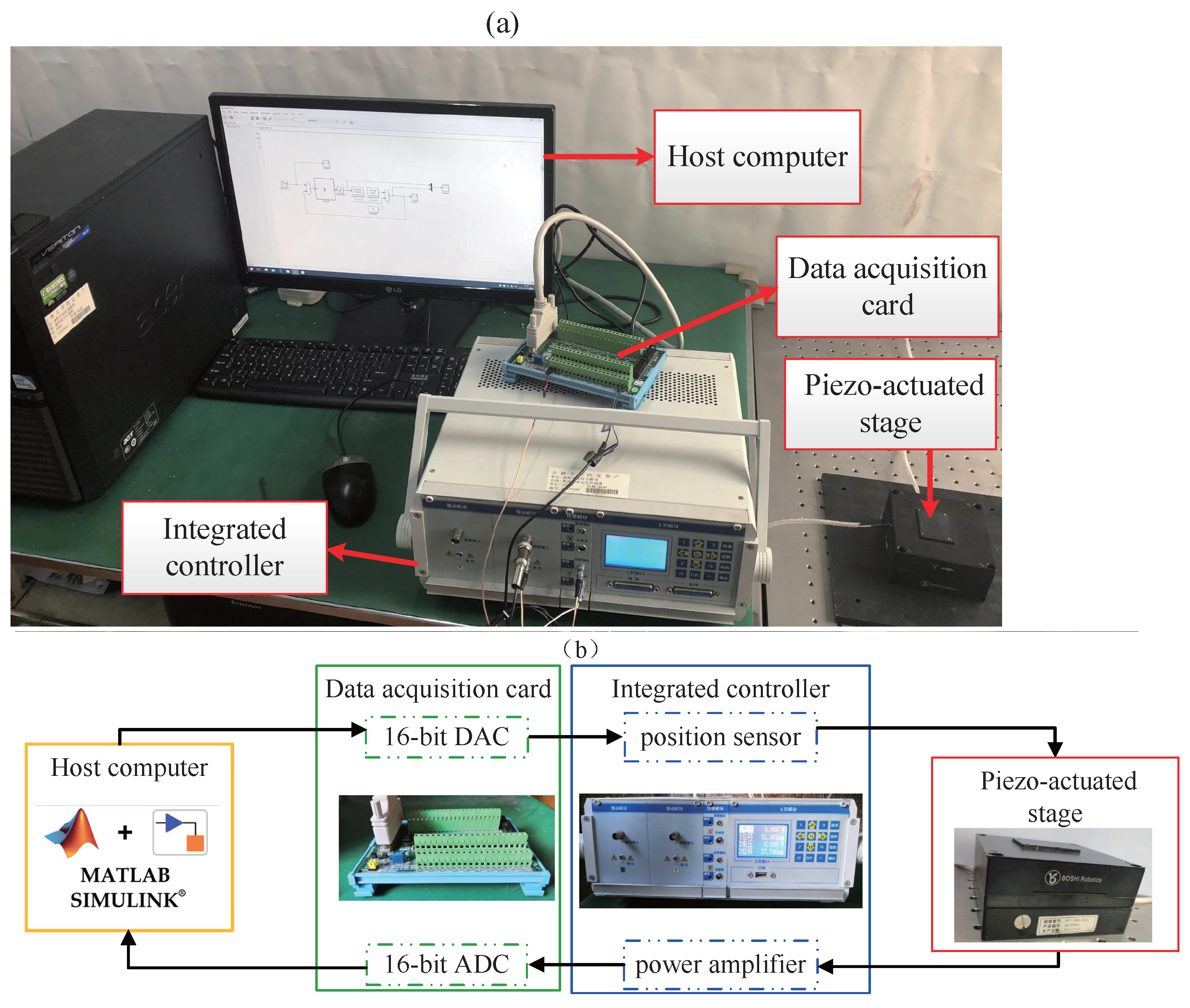
4.1. Experimental Setup

To validate the established Hammerstein model and the proposed control approach for P-AS, a series of experiments was conducted using the experimental testbed shown in Figure 3, which included a host computer (4 GB of RAM and [email protected] GHz) and a P-AS. The travel range of the P-AS was 0–50 $\mathsf{\mu }$m, the displacement resolution was 5 nm, and the operating voltage was 0–150 V. Additionally, the testbed included an integrated controller (PPC-2CR0150) and a data-acquisition card (PCI-1716). The proposed Hammerstein model and HAC based on the hysteresis compensator were implemented through the MATLAB software installed on the computer, where the sampling frequency of the system was 10 kHz. The data acquisition card converts the digital signal output from the computer into an analog signal and outputs it as a digital signal. The integrated controller amplified the analog signal as a current–voltage to drive the P-AS. A strain-type displacement sensor in the P-AS measures the current displacement and transmits it to the computer via the analog-to-digital conversion module of the data-acquisition card.

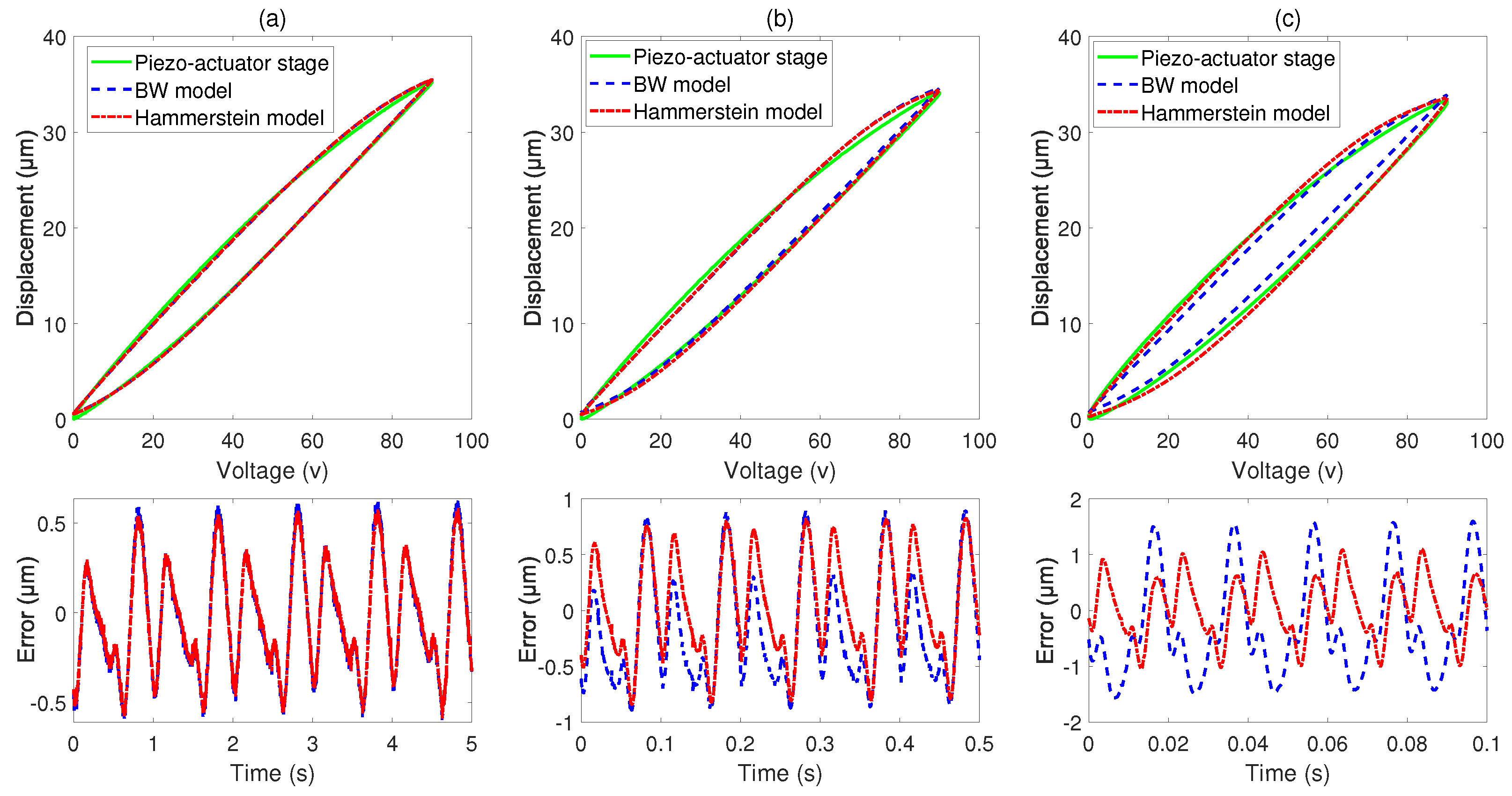
4.2. Modeling Results

The validity of the Hammerstein model was verified by comparing it with the BW model. Sinusoidal input voltages with different frequencies and an amplitude of 90 V were employed. The results are shown in Figure 4. The maximum absolute error (MAXAE) and mean absolute error (MAE) were calculated via (31) and (32), respectively. K represents a total number of sampling points. $y\left(k\right)$ and $y_m\left(k\right)$ represent the actual output and model output at the k-th sampling point, respectively. The error analysis of the BW model and the Hammerstein model are presented in

Table 1. The MAXAE and MAE of BW model and Hammerstein model.

Frequency (Hz)	MAXAE of the BW Model/ the Hammerstein Model (μm)	MAE of the BW Model/ the Hammerstein Model (μm)	Im. % (MAXAE/MAE)
1	0.6349/0.5896	0.3016/0.2847	7.13/5.60
10	0.9114/0.8455	0.5173/0.4469	7.23/13.61
50	2.0004/0.9517	1.2085/0.4669	52.42/61.36

Im.: Hammerstein model precision improvement relative to BW model.

. The MAXAEs of the Hammerstein model were 0.5896, 0.8455, and 0.9517 $\mathsf{\mu }$m, respectively, which were reduced by 7.13%, 7.23%, and 52.42% compared with those of the BW model. In addition, the MAEs of the proposed model were 0.2847, 0.4469, and 0.4669 $\mathsf{\mu }$m, respectively, which were reduced by 5.60%, 13.61%, and 61.36% compared with those of the BW model.

This indicates that the presented Hammerstein model can approximate the RD hysteresis characteristic of P-AS more accurately than the BW model.

$$e_{MAXAE}=max\left(y\left(k\right)-y_m\left(k\right)\right)$$

(31)

$$e_{MAE}=\frac{{\sum }_{k=1}^K\left|y\left(k\right)-y_m\left(k\right)\right|}{K}$$

(32)

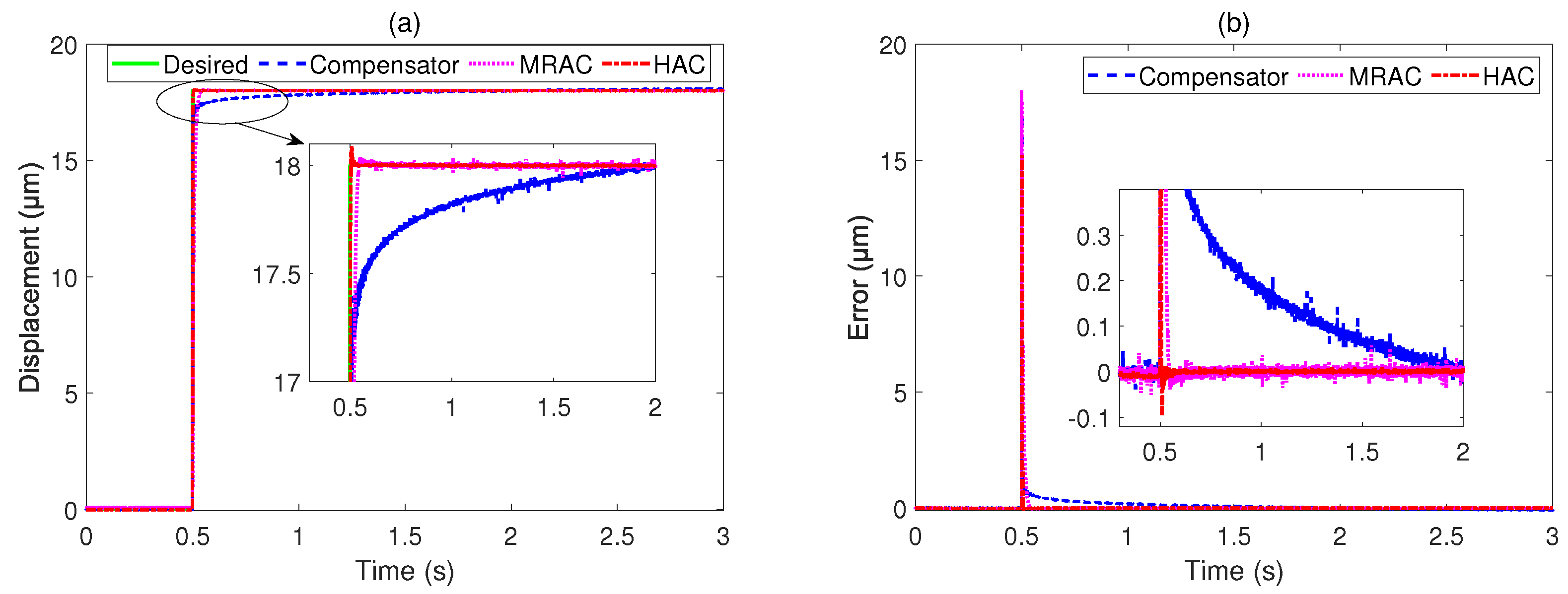
4.3. Tracking Performance under Step Response Input Signal

A step response input signal with a sudden increase from 0 to 18 $\mathsf{\mu }$m at 0.5 s was adopted as the reference trajectory to verify the tracking performance of the raised control approach. The experimental results in Figure 5 demonstrate that the raised controller had better performance than the compensator based on the inverse BW model and the MRAC. It is also evident from the experimental results that the steady-state error of the proposed controller was close to zero and has a shorter settling time compared to the MRAC and the compensator based on the inverse BW model.

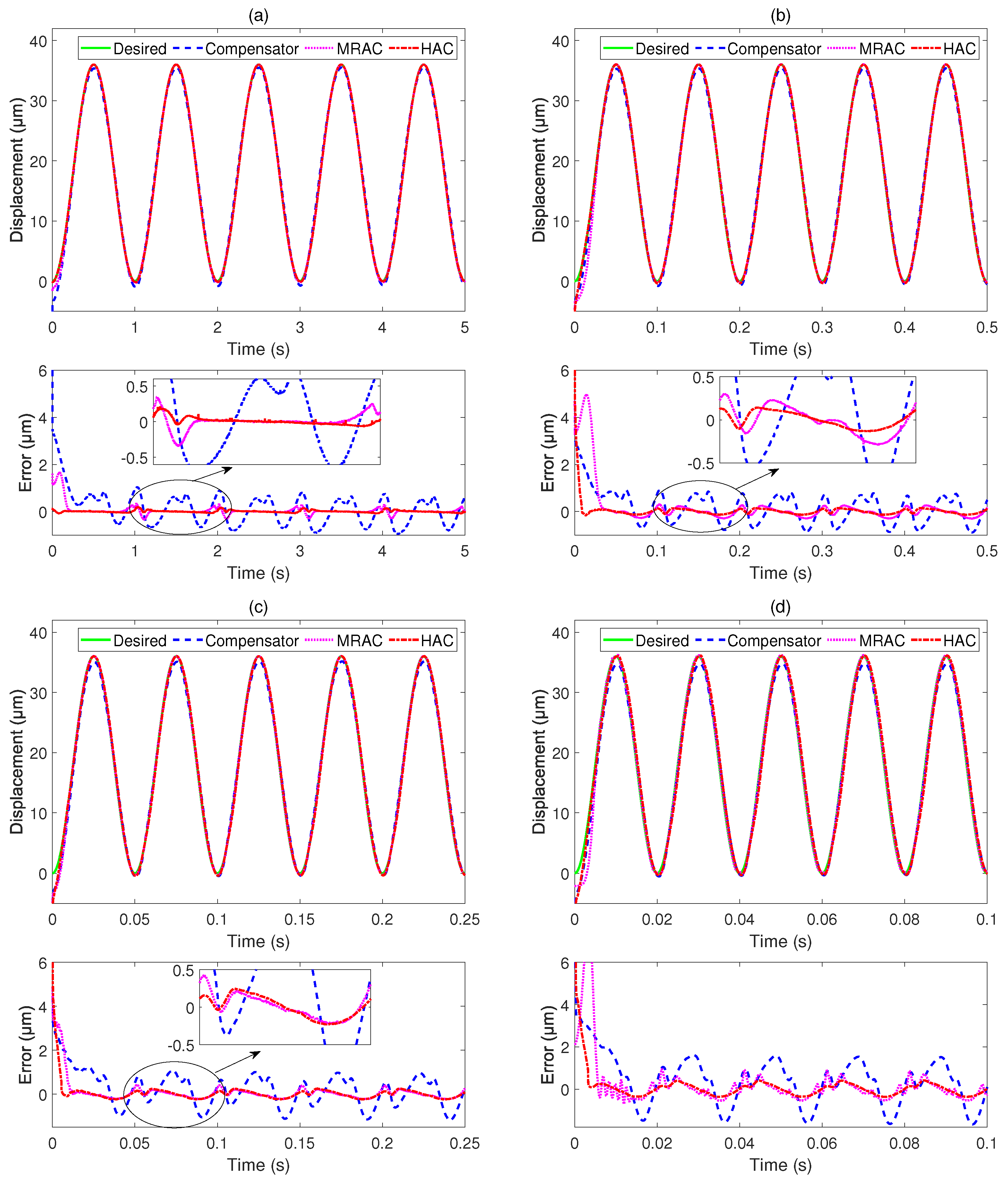
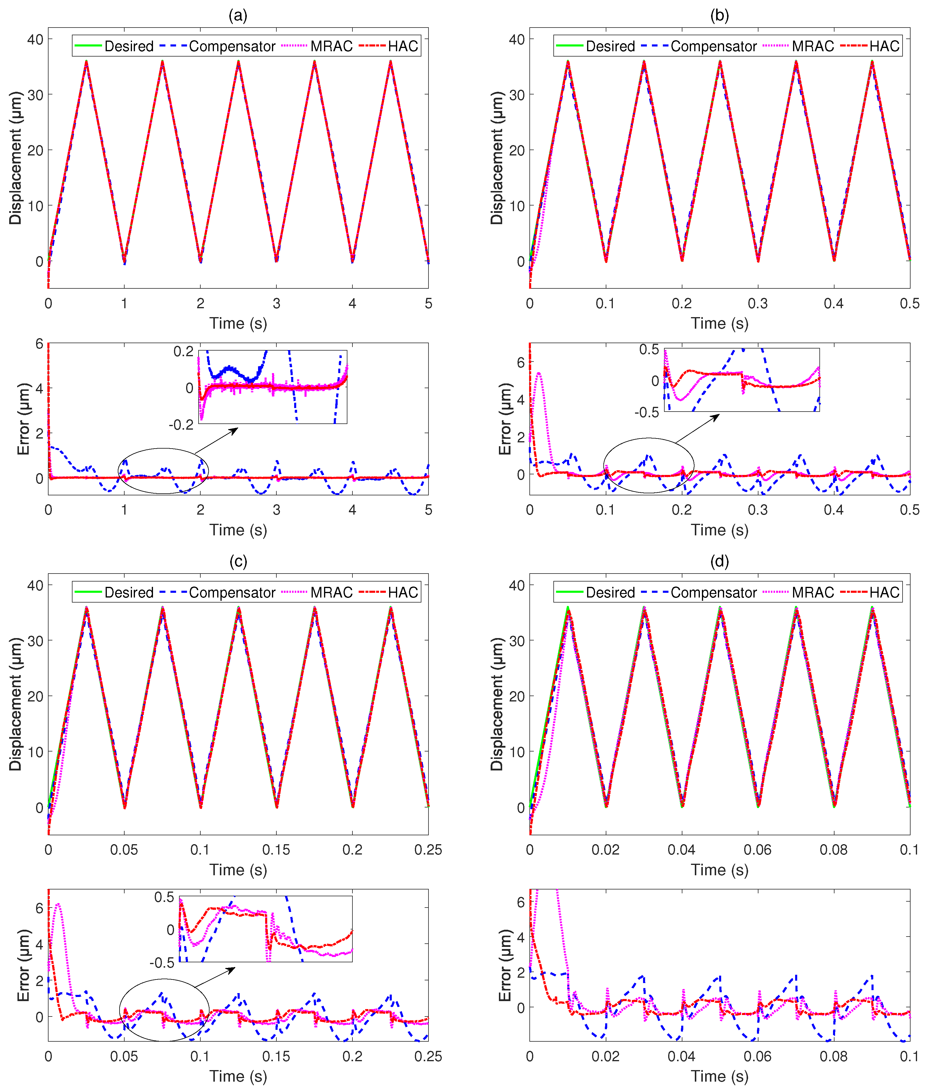
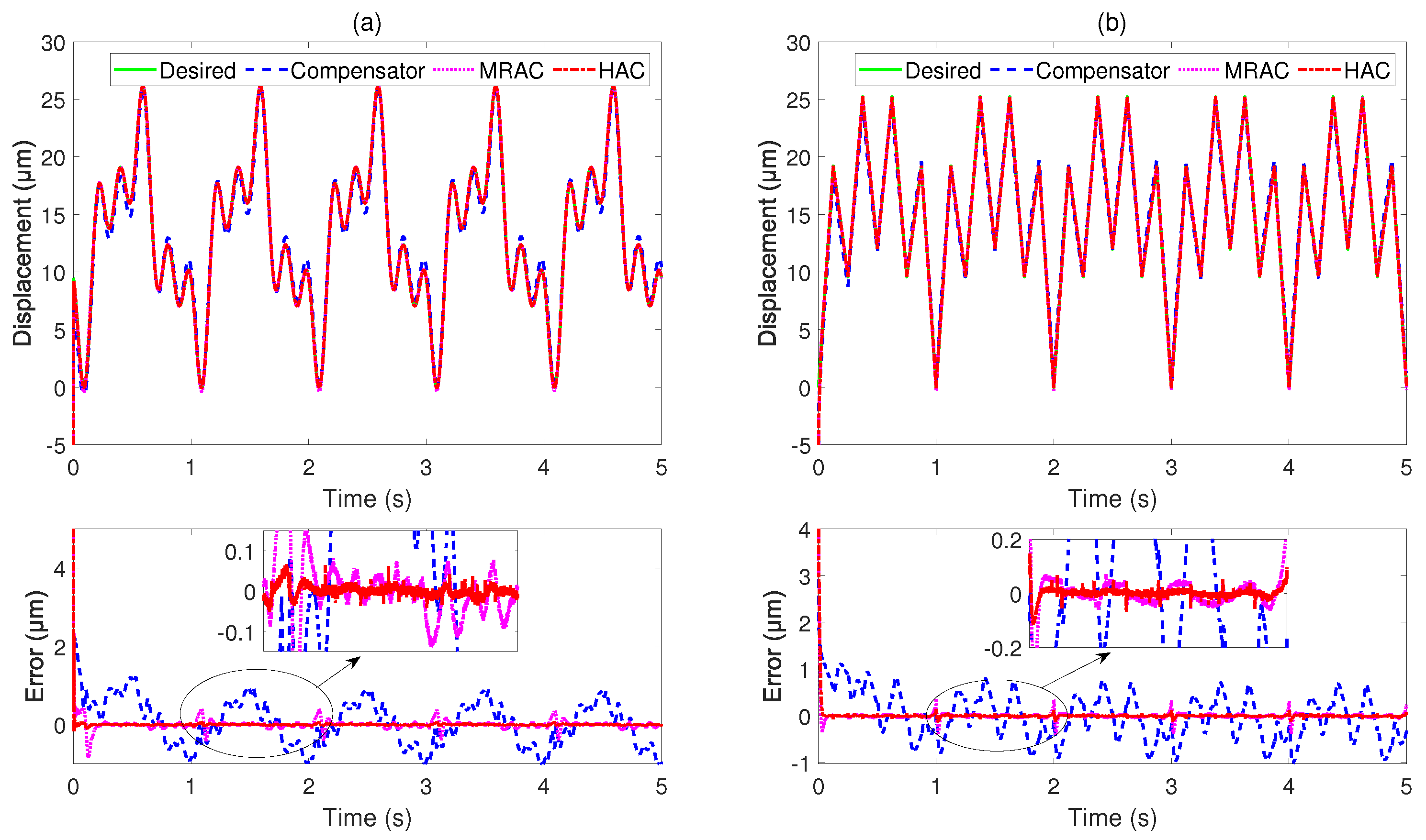
4.4. Tracking Performance under Different Reference Trajectories

Then, the tracking performance was evaluated with different reference trajectories. Sinusoidal and triangular reference signals with different frequencies (f = 1, 10, 20, and 50 Hz) were adopted. All the signals had amplitudes of 36 $\mathsf{\mu }$m. The results are shown in Figure 6 and Figure 7, and the results of quantitative analysis are presented in

Table 2. Tracking performance of different controllers under different reference trajectories.

Reference Trajectories	Frequency (Hz)	MAXAE/MAE of the Compensator (μm)	MAXAE/MAE of the MRAC (μm)	MAXAE/MAE of the Proposed Method (μm)
Sinusoidal	1	0.9522/0.4930	0.2976/0.0523	0.1748/0.0357
signal	10	0.8934/0.4968	0.3078/0.1400	0.1509/0.0803
	20	1.1772/0.5604	0.3949/0.1336	0.2607/0.1318
	50	1.6635/0.8371	0.8603/0.2919	0.4150/0.2122
Triangular	1	0.7741/0.2678	0.1603/0.0141	0.0659/0.0088
signal	10	1.1250/0.5689	0.3862/0.1129	0.1707/0.0939
	20	1.3742/0.7145	0.6140/0.2792	0.3488/0.2250
	50	1.9488/0.9441	0.9414/0.3617	0.4296/0.3165

. The tracking error was evaluated according to the MAXAE and MAE via (31) and (32), respectively. $Z_d\left(k\right)=y_r\left(k\right)$ and $Z\left(k\right)=y\left(k\right)$ represent the actual and desired outputs of the P-AS, respectively. All the MAXAEs and MAEs for the proposed control method were smaller than those for the compensator based on the inverse BW model and MRAC under sinusoidal and triangular reference signals with frequencies of 1, 10, 20, and 50 Hz. In particular, the MAE of the raised controller was 66.5% and 12.5% smaller than those of the compensator and MRAC, respectively, for the 50 Hz sinusoidal reference trajectory.

Compared with the adopted sliding mode tracking control adopted in [36], the HAC method improves the control effect significantly. When the frequency of the triangular reference signals was 1 and 10 Hz, the proposed control method attenuated the MAE from 1.18% and 1.96% to 0.02% and 0.26%, respectively. In addition, the MAE of the HAC method was smaller than that of the neural-network self-tuning control raised in [50]. When the frequency of the sinusoidal reference signals was 1, 10, and 20 Hz, the proposed control method reduced the MAE from 1.02%, 1.26%, and 1.85% to 0.49%, 0.42%, and 0.72%, respectively.

Figure 8 shows a further evaluation of the tracking performance with different complex reference trajectories. Figure 8a presents a comparison of the tracking results with the desired mixed sinusoidal signal. As shown, the tracking errors of the raised control approach were significantly smaller than those of the compensator and MRAC. Figure 8b presents a comparison of the tracking results with the desired mixed triangular signal. As shown, the MAE of the proposed control method was 0.0095 $\mathsf{\mu }$m, which was 97.6% and 74.1% smaller than those of the compensator and MRAC, respectively. The experimental results also show that the proposed control method has better control performance for both complex harmonic wave signal and triangular signal. In addition, the proposed control method can better suppress the effect of hysteresis on the accuracy of the P-AS at the peak point of the tracking signal.

5. Conclusions

A hysteresis modeling and compensation method for P-AS was developed. We propose a Hammerstein model comprising a BW static hysteresis sub-model and a dynamic linear sub-model. An improved differential evolution algorithm and a least-squares algorithm are used to identify the static hysteresis sub-model and dynamic linear sub-model for the Hammerstein model, respectively. To suppress the influence of hysteresis on the precision of P-AS, a hysteresis controller based on the inverse BW model was designed to depress the static hysteresis of the stage. However, modeling errors, environmental noise, and measurement errors also reduce the control accuracy. To resolve these complications, a HAC method based on a hysteresis compensator is proposed for increasing the control accuracy. By constructing a reference model of the system and considering the unmodeled dynamics at the input and output, the effects of model uncertainty and perturbations on the system accuracy can be significantly reduced. With the help of the Lyapunov stability theory, the stability of the system is proved. Finally, the effectiveness of the raised approach was verified by a series of experiments involving comparisons with the hysteresis compensation controller based on the inverse BW model and MRAC. The experimental results indicated that the HAC method is efficient for the precise positioning of P-AS.

References

1. Ho, S.T.; Jan, S.J. A piezoelectric motor for precision positioning applications. Precis. Eng. 2016, 43, 285–293. [Google Scholar] [CrossRef]
2. Shao, J.; Chen, X.; Li, X.; Tian, H.; Wang, C.; Lu, B. Nanoimprint lithography for the manufacturing of flexible electronics. Sci. China Technol. Sci. 2019, 62, 175–198. [Google Scholar] [CrossRef]
3. Xu, R.; Pan, W.; Wang, Z.; Tian, D. High-precision tracking control of a piezoelectric micro/nano platform using sliding mode control with the fractional-order operator. Int. J. Precis. Eng. Manuf. 2020, 21, 2277–2286. [Google Scholar] [CrossRef]
4. Clark, L.; Shirinzadeh, B.; Zhong, Y.; Tian, Y.; Zhang, D. Design and analysis of a compact flexure-based precision pure rotation stage without actuator redundancy. Mech. Mach. Theory 2016, 105, 129–144. [Google Scholar] [CrossRef]
5. Do, T.N.; Tjahjowidodo, T.; Lau, M.; Yamamoto, T.; Phee, S.J. Hysteresis modeling and position control of tendon-sheath mechanism in flexible endoscopic systems. Mechatronics 2014, 24, 12–22. [Google Scholar] [CrossRef]
6. Wang, Y.; Zhou, M.; Shen, C.; Cao, W.; Huang, X. Time delay recursive neural network-based direct adaptive control for a piezo-actuated stage. Sci. China Technol. Sci. 2022; accepted. [Google Scholar]
7. Xu, R.; Tian, D.; Wang, Z. Adaptive Tracking Control for the Piezoelectric Actuated Stage Using the Krasnosel’skii-Pokrovskii Operator. Micromachines 2020, 11, 537. [Google Scholar] [CrossRef]
8. Pota, H.R.; Ian, R.P.; Rana, M.S. Creep, hysteresis, and cross-coupling reduction in the high-precision positioning of the piezoelectric scanner stage of an atomic force microscope. IEEE Trans. Nanotechnol. 2013, 12, 1125–1134. [Google Scholar]
9. Zhang, C.; Yu, Y.; Xu, J.; Zhou, M. Hysteresis modeling and analysis of magnetic shape memory alloy-driven actuator. IEEE Trans. Nanotechnol. 2022, 21, 390–398. [Google Scholar] [CrossRef]
10. Xu, R.; Tian, D.; Zhou, M. A rate-dependent KP modeling and direct compensation control technique for hysteresis in piezo-nanopositioning stages. J. Intell. Mater. Syst. Struct. 2022, 33, 629–640. [Google Scholar] [CrossRef]
11. Bouc, R. Forced vibrations of mechanical systems with hysteresis. In Proceedings of the 4th Conference Nonlinear Oscillation, Prague, Czech Republic, 5–9 September 1967. [Google Scholar]
12. Wen, Y. Method for random vibration of hysteretic systems. J. Eng. Mech. Div. 1976, 102, 249–263. [Google Scholar] [CrossRef]
13. Nguyen, P.B.; Choi, S.B.; Song, B.K. A new approach to hysteresis modelling for a piezoelectric actuator using Preisach model and recursive method with an application to open-loop position tracking control. Sens. Actuators A Phys. 2018, 270, 136–152. [Google Scholar] [CrossRef]
14. Xu, Q. Precision motion control of piezoelectric nanopositioning stage with chattering-free adaptive sliding mode control. IEEE Trans. Autom. Sci. Eng. 2017, 14, 238–248. [Google Scholar] [CrossRef]
15. Tan, X.; Baras, J.S. Modeling and control of hysteresis in magnetostrictive actuators. Automatica 2004, 40, 1469–1480. [Google Scholar] [CrossRef] [Green Version]
16. Lin, C.J.; Lin, P.T. Tracking control of a biaxial piezo-actuated positioning stage using generalized Duhem model. Comput. Math. Appl. 2012, 64, 766–787. [Google Scholar] [CrossRef] [Green Version]
17. Su, C.Y.; Stepanenko, Y.; Svoboda, J.; Leung, T.P. Robust adaptive control of a class of nonlinear systems with unknown backlash-like hysteresis. IEEE Trans. Autom. Control 2000, 45, 2427–2432. [Google Scholar] [CrossRef] [Green Version]
18. Habineza, D.; Rakotondrabe, M.; Gorrec, Y. Bouc-Wen modeling and feedforward control of multivariable hysteresis in piezoelectric systems: Application to a 3-DoF piezotube scanner. IEEE Trans. Control. Syst. Technol. 2015, 14, 1797–1806. [Google Scholar] [CrossRef]
19. Rakotondrabe, M. Bouc-Wen modeling and inverse multiplicative structure to compensate hysteresis nonlinearity in piezoelectric actuators. IEEE Trans. Autom. Sci. Eng. 2011, 8, 428–431. [Google Scholar] [CrossRef] [Green Version]
20. Zhou, M.; Wang, Y.; Zhang, Y.; Gao, W. Hysteresis inverse compensation-based model reference adaptive control for a piezoelectric micro-positioning platform. Smart Mater. Struct. 2020, 30, 015019. [Google Scholar] [CrossRef]
21. Song, G.; Zhao, J.; Zhou, X.; Abreu-Garcia, J.A. Tracking control of a piezoceramic actuator with hysteresis compensation using inverse Preisach model. IEEE/ASME Trans. Mechatron. 2005, 10, 198–209. [Google Scholar] [CrossRef]
22. Li, Z.; Zhang, X.; Su, C.Y.; Chai, T. Nonlinear control of systems preceded by Preisach hysteresis description: A prescribed adaptive control approach. IEEE Trans. Control. Syst. Technol. 2016, 24, 451–460. [Google Scholar] [CrossRef]
23. Gan, J.; Zhang, X.; Wu, H. A generalized Prandtl-Ishlinskii model for characterizing the rate-independent and rate-dependent hysteresis of piezoelectric actuators. Rev. Sci. Instrum. 2016, 87, 035002. [Google Scholar] [CrossRef] [PubMed]
24. Yang, M.; Li, C.; Gu, G.; Zhu, L. Modeling and compensating the dynamic hysteresis of piezoelectric actuators via a modified rate-dependent Prandtl-Ishlinskii model. Smart Mater. Struct. 2015, 24, 125006. [Google Scholar] [CrossRef]
25. Nie, L.; Luo, Y.; Gao, W.; Zhou, M. Rate-dependent asymmetric hysteresis modeling and robust adaptive trajectory tracking for piezoelectric micropositioning stages. Nonlinear Dyn. 2022, 108, 2023–2043. [Google Scholar] [CrossRef]
26. Li, Z.; Shan, J.; Gabbert, U. Inverse compensation of hysteresis using Krasnoselskii-Pokrovskii model. IEEE/ASME Trans. Mechatron. 2018, 23, 966–971. [Google Scholar] [CrossRef]
27. Liu, Y.; Zhou, M. KP model for hysteresis of piezoelectric ceramic actuators. In Proceedings of the 2015 Chinese Automation Congress (CAC), Wuhan, China, 27–29 November 2015; pp. 27–29. [Google Scholar]
28. Xu, R.; Zhou, M. Elman neural network-based identification of Krasnoselskii-Pokrovskii model for magnetic shape memory alloys actuator. IEEE Trans. Magn. 2017, 53, 2002004. [Google Scholar] [CrossRef]
29. Gan, J.; Zhang, X. A review of nonlinear hysteresis modeling and control of piezoelectric actuators. AIP Adv. 2019, 9, 040702. [Google Scholar] [CrossRef] [Green Version]
30. Landis, C.; Zhou, M. Non-linear constitutive modeling of ferroelectrics. Curr. Opin. Solid State Mater. Sci. 2004, 8, 59–69. [Google Scholar] [CrossRef]
31. Delibas, B.; Arockiarajan, A.; Seemann, W. Rate dependent properties of perovskite type tetragonal piezoelectric materials using micromechanical model. Int. J. Solids Struct. 2006, 43, 697–712. [Google Scholar] [CrossRef] [Green Version]
32. Zhang, X.; Wang, Y.; Wang, C.; Su, C.Y.; Li, Z.; Chen, X. Adaptive estimated inverse output-feedback quantized control for piezoelectric positioning stage. IEEE Trans. Cybern. 2019, 49, 2106–2118. [Google Scholar] [CrossRef]
33. Xie, S.; Liu, H.; Wang, Y. A method for the length-pressure hysteresis modeling of pneumatic artificial muscles. Sci. China Technol. Sci. 2020, 63, 829–837. [Google Scholar] [CrossRef]
34. Li, Z.; Shan, J.; Gabbert, U. Dynamics modeling and inversion-based synchronized model predictive control for a Fabry-Perot spectrometer. IEEE/ASME Trans. Mechatron. 2019, 24, 1818–1828. [Google Scholar] [CrossRef]
35. Xu, Q.; Li, Y. Dahl model-based hysteresis compensation and precise positioning control of an XY parallel micromanipulator with piezoelectric actuation. J. Dyn. Syst. Meas. Control 2010, 132, 042011. [Google Scholar] [CrossRef]
36. Xu, R.; Zhang, X.; Guo, H.; Zhou, M. Sliding mode tracking control with perturbation estimation for hysteresis nonlinearity of piezo-actuated stages. IEEE Access 2018, 6, 30617–30629. [Google Scholar] [CrossRef]
37. Feng, Z.; Liang, W.; Ling, J.; Xiao, X.; Tan, K.K.; Lee, T.H. Integral terminal sliding-mode-based adaptive integral backstepping control for precision motion of a piezoelectric ultrasonic motor. Mech. Syst. Signal Process. 2020, 144, 27–29. [Google Scholar] [CrossRef]
38. Yu, Y.; Zhang, C.; Cao, W.; Huang, X.; Zhang, X.; Zhou, M. Neural network based iterative learning control for magnetic shape memory alloy actuator with iteration-dependent uncertainties. Mech. Syst. Signal Process. 2023, 187, 109950. [Google Scholar] [CrossRef]
39. Yu, Y.; Zhang, C.; Wang, Y.; Zhou, M. Neural-network-based iterative learning control for hysteresis in a magnetic shape memory alloy actuator. IEEE/ASME Trans. Mechatron. 2021, 27, 928–939. [Google Scholar] [CrossRef]
40. Wang, Y.; Zhou, M.; Hou, D.; Cao, W.; Huang, X. Composite data driven-based adaptive control for a piezoelectric linear motor. IEEE Trans. Instrum. Meas. 2022, 71, 3527912. [Google Scholar] [CrossRef]
41. Wang, X.S.; Su, C.Y.; Hong, H. Robust adaptive control of a class of nonlinear systems with unknown dead-zone. Automatica 2004, 40, 407–413. [Google Scholar] [CrossRef]
42. Ahamd, I.; Abdurraqeeb, A.M. H control design with feed-forward compensator for hysteresis compensation in piezoelectric actuators. Automatica 2019, 57, 691–702. [Google Scholar] [CrossRef] [Green Version]
43. Liu, W.; Cheng, L.; Hou, Z.G.; Yu, J.; Tan, M. An inversion-free predictive controller for piezoelectric actuators based on a dynamic linearized neural network model. IEEE/ASME Trans. Mechatron. 2016, 21, 214–226. [Google Scholar] [CrossRef]
44. Cheng, L.; Liu, W.; Hou, Z.G.; Yu, J.; Tan, M. Neural-network-based nonlinear model predictive control for piezoelectric actuators. IEEE Trans. Ind. Electron. 2015, 62, 7717–7727. [Google Scholar] [CrossRef]
45. Li, C.; Gu, G.; Yang, M.; Zhu, L. High-speed tracking of a nanopositioning stage using modified repetitive control. IEEE Trans. Autom. Sci. Eng. 2017, 14, 1467–1477. [Google Scholar] [CrossRef]
46. Zhang, C.; Yu, Y.; Wang, Y.; Zhou, M. Takagi-Sugeno fuzzy neural network hysteresis modeling for magnetic shape memory alloy actuator based on modified bacteria foraging algorithm. Int. J. Fuzzy Syst. 2020, 22, 1314–1329. [Google Scholar] [CrossRef]
47. Qin, Y.; Tian, Y.; Zhang, D.; Shirinzadeh, B.; Fatikow, S. A novel direct inverse modeling approach for hysteresis compensation of piezoelectric actuator in feedforward applications. IEEE/ASME Trans. Mechatron. 2013, 18, 981–989. [Google Scholar] [CrossRef]
48. Lavretsky, E. Combined/composite model reference adaptive control. IEEE Trans. Autom. Sci. Eng. 2009, 54, 2692–2697. [Google Scholar] [CrossRef]
49. Zhang, X.; Chen, X.; Zhu, G.; Su, C.Y. Output feedback adaptive motion control and its experimental verification for time-delay nonlinear systems with asymmetric hysteresis. IEEE Trans. Ind. Electron. 2020, 67, 6824–6834. [Google Scholar] [CrossRef]
50. Li, W.; Zhang, C.; Gao, W.; Zhou, M. Neural network self-tuning control for a piezoelectric actuator. Sensors 2020, 20, 3342. [Google Scholar] [CrossRef]
Figure 1. Schematic diagram of the Hammerstein model.
Applsci 13 00402 g001
Figure 2. Structure of the proposed hybrid adaptive controller.
Applsci 13 00402 g002
Figure 3. (a) Picture of the experimental testbed. (b) Schematic of the experimental testbed.
Applsci 13 00402 g003
Figure 4. Modeling results of the Hammerstein model in comparison with the BW model under sinusoidal input voltages of different frequencies: (a) modeling result at frequency of 1 Hz; (b) modeling result at frequency of 10 Hz; (c) modeling result at frequency of 50 Hz.
Applsci 13 00402 g004
Figure 5. Tracking performance of the HAC method in comparison with the compensator and MRAC under step response input signal: (a) control results; (b) tracking errors.
Applsci 13 00402 g005
Figure 6. Tracking performance of the HAC method in comparison with the compensator and MRAC under sinusoidal reference trajectories of different frequencies: (a) tracking result at frequency of 1 Hz; (b) tracking result at frequency of 10 Hz; (c) tracking result at frequency of 20 Hz; (d) tracking result at frequency of 50 Hz.
Applsci 13 00402 g006
Figure 7. Tracking performance of the HAC approach in comparison with the compensator and MRAC under triangular reference trajectories of different frequencies: (a) tracking result at frequency of 1 Hz; (b) tracking result at frequency of 10 Hz; (c) tracking result at frequency of 20 Hz; (d) tracking result at frequency of 50 Hz.
Applsci 13 00402 g007
Figure 8. Tracking performance of the HAC approach in comparison with the compensator and MRAC under different complex reference trajectories: (a) mixed sinusoidal signal; (b) mixed triangular signal.
Applsci 13 00402 g008