Multiple Pedestrian Tracking in Dense Crowds Combined with Head Tracking

Abstract

In order to reduce the negative impact of severe occlusion in dense scenes on the performance degradation of the tracker, considering that the head is the highest and least occluded part of the pedestrian’s entire body, we propose a new multiobject tracking method for pedestrians in dense crowds combined with head tracking. For each frame of the video, a head tracker is first used to generate the pedestrians’ head movement tracklets, and the pedestrians’ whole body bounding boxes are detected at the same time. Secondly, the degree of association between the head bounding boxes and the whole body bounding boxes are calculated, and the Hungarian algorithm is used to match the above calculation results. Finally, according to the matching results, the head bounding boxes in the head tracklets are replaced with the whole body bounding boxes, and the whole body motion tracklets of the pedestrians in the dense scene are generated. Our method can be performed online, and experiments suggested that our method effectively reduces the negative effects of false negatives and false positives on the tracker caused by severe occlusion in dense scenes.

1. Introduction

Multiple-object tracking (MOT) is a kind of general algorithm that can be applied in various fields of computer vision, such as video surveillance, autonomous driving, human–computer interaction, and the medical field. In these scenarios, we can use MOT algorithms to compute the positions, shapes, speeds, trajectories and other information of targets in tracked videos, and further accomplish the functions of object behaviour analysis or object counting. In addition, the reliable motion tracklets generated by MOT algorithms could also effectively compensate for the missed detections in object-detection tasks, and help the detectors to perform more accurately.

In the real MOT tasks in dense crowds, occlusions among pedestrians are always very difficult for trackers. This phenomenon is manifested when the view of some pedestrians is completely or partially covered by other pedestrians who are closer to the camera. Occlusions make it difficult to perceive pedestrians’ visual clues, i.e., the information of targets is lost. The key to the tracking algorithm is to gather enough target information to determine where the targets are, and assign a unique ID for each target. Therefore, occlusions expose a great number of challenges to the reliability for pedestrian tracking, which may lead to unstable tracklets and even loss of targets. These phenomena cause the rise of some metrics, such as mostly lose (ML), false negative (FN), false positive (FP), identity switch (IDSw), and other indicators for MOT, and the decline of indicators, such as multiple object-tracking accuracy (MOTA), ID F1 score (IDF1), and higher-order tracking accuracy (HOTA). To the researchers of MOT algorithms, this is not what they expect to see.

Compared with the general MOT scenes, the huge number of targets in the dense crowd leads to more serious mutual occlusions among the targets, because the frequency and coverage of occlusions in the dense crowd become more critical. This phenomenon is manifested in the real video recordings that the target A in the video blocks another target B, and the target B blocks the target C at the same time. These layer-by-layer occlusions cause the relationship among the targets to become more chaotic, and bring more instability for the MOT task. The way to effectively handle occlusions, especially severe and frequent occlusions in dense crowds, has always been a difficult issue for MOT tasks in crowds. At present, most MOT systems cannot deal with serious occlusion problems, nor can they provide criteria for judging when to terminate the unconfirmed tracklets and when to restart the killed tracklets of targets, and there is no corresponding guidance method to reobtain the targets when they are lost.

In conventional MOT algorithms, rather than any single part of the target, researchers directly select the entire target as the object to be tracked. Those methods, as the current mainstream research methods [1,2,3,4,5,6], had indeed achieved considerable results. However, when conducting multiobject research in dense crowds, the effectiveness of those methods will be greatly reduced. As mentioned above, the relationships among the targets in dense crowds are extremely chaotic. One target is likely to block several other targets, causing the motion and appearance features of these targets to be lost in overwhelming quantities. The trackers cannot capture enough valid information, which leads to a significant drop in their performance.

The head is the highest and least occluded part of a pedestrian. It is reflected that in dense crowd scenes, the detector for heads can detect a large number of heads, but the detector for full bodies cannot. As shown in Figure 1, in this picture, the head detector has successfully located and recognized the majority of heads, but the full body detector fails. Furthermore, compared to the pedestrian’s entire body, the head has a smaller size, which indicates that even if some heads are occluded in some frames, they are more likely to reappear soon due to the fact that they only occupy small areas in the entire frame. Fortunately, the trackers tend to recover the tracklets of short-term occluded targets. In short, the head has become an ideal object to track. Therefore, using the head to track instead of body tracking in dense crowds can reduce the negative effects of severe occlusions to a considerable extent.

Figure 1. On the premise of inputting the same picture, the head detector used in our approach detects 64 head bounding boxes, whereas a general full-body detector (which is an original implementation of Faster-RCNN) can only detect 46 of the 71 targets.

In order to solve the problem of poor performance of multiple pedestrian trackers in dense crowd, and considering that the head is more suitable as a tracking object for MOT tasks in dense crowds, we proposed a novel approach for multiple pedestrian tracking in dense crowds combined with head tracking, and we named it as Tracking Pedestrians with Head Tracker (TraPeHat). Our method matched the head bounding boxes with the whole-body bounding boxes on the basis of obtaining the head movement tracklets, and replaced the head bounding boxes in the head tracklets with the whole-body bounding boxes according to the matching results to generate the final full-body trajectories. On the basis of ensuring the tracking accuracy, our method effectively reduced the number of false negatives and false positives caused by occlusions, and improved the actual performance of the multiobject tracker in dense crowds. It demonstrated certain practical values because it can be placed in many venues, such as airports, stations, gymnasiums, shopping centers, crossroads, etc. An official implementation of our paper can be found in https://github.com/TUT103/THT.git (accessed on 23 December 2022).

Our paper has the following contributions.

• Inheriting the work of [7], which only tracks the pedestrians’ heads, we extended the tracked objects to the whole bodies of pedestrians, which are more common in the field of multiobject tracking.
• To accomplish the task of matching pedestrians’ head and body bounding boxes, we proposed a novel bounding box similarity calculation method, Intersection over Containment (IoC), by which, with the help of the Hungarian algorithm, we can efficiently complete the matching work of the head bounding box and the whole-body bounding box belonging to the same pedestrian.
• We used the MOT20 [8], SCUT-Head [9], HT21 [7], and CrowdHuman [10] datasets to conduct a series of related experiments to demonstrate the feasibility and effectiveness of the above methods.

2. Related Work

2.1. Tracking by Detection

Tracking by detection (TDB) is a common paradigm in the MOT field. TDB has the characteristics of high accuracy, relatively fast speed, and real-time performance. It has been the mainstream method in the field of MOT in the past.

The detection algorithm is the cornerstone of the operation of the TDB paradigm. The addition of the convolutional neural network (CNN) [11] enabled the detection algorithms to achieve rapid development in both detection accuracy and running speed [12,13,14,15,16,17,18,19]. Powerful detection algorithms could be introduced to TDB trackers to obtain better tracking performance. RetinaNet was a typical object detector essentially composed of CNN plus feature pyramid networks (FPN) [20] plus two fully convolutional networks (FCN) [21]. By using the loss function focal loss, the weights of samples that are difficult to classify were increased, and the ratios of positive and negative samples were effectively controlled. RetinaNet was used by various MOT algorithms, such as RetinaTrack [22] and Chained Tracker [23]. The version of You Only Look Once (YOLO) [24] detectors had gone through from V1 to V5, and the latest YOLO version detectors generally achieved good balance between accuracy and speed, and it was used by a large number of methods [25,26,27]. There are many improved versions in the follow-up, and the best performance is You Only Look Once X (YOLOX) [28], which is a very popular detector at present. CenterNet [29] abandoned the widely used anchors in traditional detection algorithms, and derived the center points, widths, heights, offsets, and other information of the targets by introducing heat map, and used the anchor-free method to obtain the bounding boxes of the targets. CenterNet had also been widely used due to its simplicity and efficiency [30,31,32,33,34]. In general, the vast majority of trackers only implement MOT algorithms through the bounding boxes from the current frames.

DeepSort [35] is a classic MOT algorithm that complies with the TDB paradigm, and it was improved from the SORT algorithm. In order to predict the trajectories of the targets, researchers usually use state estimation filters, like the Kalman filter [36] and Alpha–Beta filter [37,38]. Before running DeepSort, it is helpful to use an independent detector like YOLOV3 to detect the targets of interest in each frame of the video, then use the Kalman filter, Hungarian algorithm [39], feature extractor, and other components to comprehensively consider the motion law, appearance similarity, motion similarity, and other information of the target bounding boxes, with the step of Kalman prediction, matching, and Kalman updating to calculate the target motion tracklets. DeepSort runs fast, can meet real-time requirements, and has high accuracy, so it is one of the most widely used MOT algorithms in the industry at present. There are many improved versions of DeepSort, like MOTDT and ByteTrack. ByteTrack is a typical and well-known tracker among the improved works. In contrast to general MOT algorithms that directly discard the bounding boxes with lower confidence, ByteTrack reused the bounding boxes with lower confidence by executing the Kalman filter and Hungarian algorithm twice. The first usage was between bounding boxes with high confidence and tracklets, and the second usage was between bounding boxes with lower confidence and the unmatched tracklets in the first time. It should be noted that the reason for the low confidence of the bounding boxes is general occlusion and indistinctness, and occlusions indicate that the appearance information of those objects is mixed with other bounding boxes, so only the motion law is considered in the second matching, and the appearance information is not considered. Researchers familiar with DeepSort will soon understand ByteTrack.

2.2. Jointly Learns the Detector and Embedding

The TDB paradigm performs the detection task and tracking task separately. This kind of algorithm has good accuracy and is easy to understand, but the disadvantages are also obvious, i.e., separate execution of detection and tracking requires more reasoning time. This kind of model is not easy to achieve a real-time effect on edge devices, so the Jointly Learns the Detector and Embedding (JDE) [40,41,42] paradigm came into being.

Wang et al. earlier proposed a MOT method that integrates detection and reidentification. They fed an image frame into a backbone network with FPN to obtain multilayer prediction heads. The prediction head led to three prediction branches, namely the box classification, the box regression, and the reidentification. These three branches had their own unique loss functions, and were fused in the end. The most obvious feature of Wang’s method is its fast speed; secondly, it is easy to understand with considerable accuracy. Later, Zhang proposed his own improvements to Wang’s method, so that the advantages of JDE were further explored. Zhang input a frame into Resnet34 integrating deep layer aggregation (DLA). DLA has a large number of jump connections between low-dimensional and high-dimensional information, so the feature information can be encrypted and decrypted. The feature map was then fed into the detection branch and the reidentification branch, the detection branch output the center points, center point offsets, and bounding box sizes of the targets, and the reidentification branch was further extracted for the desired features. Zhang’s method has the following advantages. First, according to the following experiments, anchors are not suitable for the extraction of reidentification information. Zhang eliminated the negative effects caused by the anchor-free method, so that the reidentification branch was fully trained. Secondly, through multitask loss optimization, the problem of feature conflict caused by feature sharing was solved. Finally, the disadvantage of high-dimensional information on reidentification was eliminated by extracting low-dimensional information (32-dimensional), and the reasoning was accelerated, because it had been proven through experiments that extracting low-dimensional feature information in the JDE field can achieve high tracking accuracy and efficiency. JDE has gained attention by researchers due to its high accuracy and fast speed.

2.3. Tracking Method Based on Transformer

Because Transformer [43] was successfully used in natural language processing (NLP), the subsequent versions of Transformer [44,45] have been continuously shining in this field. Later, when DETR [46] was introduced as a vision variant of Transformer, researchers started to realize that Transformer also has great potential value in the MOT field. As more researchers follow up, Transformer is also fruitful in more computer vision tasks [47,48,49], like classification, segmentation, image caption, lane line detection, etc.

TransTrack [50] was the first work to use Transformer for MOT. TransTrack consisted of one encoder and two parallel decoders. The encoder input the feature map processed by CNN. The two decoders input the object query and the existing track query, respectively. The outputs of the two decoders were matched by intersection of union (IoU) to obtain the tracklets of objects’ motion.

The main difference between the main structure of TrackFormer [51] and TransTrack is that the object query and track query were input into a shared decoder in TrackFormer, and the decoder output two heads, which were the heads for classes and positions of boxes for the tracklets.

TransCenter [52] is also a piece of work that used Transformer for MOT. When TransCenter processes a frame from a video, it needs the feature maps of the current frame and the previous frame to input two parallel deformable encoders (DE) and then output the memory feature maps for the current frame ($M_t$) and previous frame ($M_{t - 1}$), respectively. Then they are sent to the query learn network (QLN) to generate dense multiscale query ($D{Q}_t$) and ($T{Q}_t$) for tracking and detection, respectively. Followed by two parallel deformable track decoders (DTD) and deformable detect decoders (DDD), respectively, for tracking and detection, DDD retrieves the current frame information from $M_t$ through $D{Q}_t$ to output multiscale detection feature ($D{F}_t$), and DTD retrieves the previous frame information from $M_{t - 1}$ through $T{Q}_t$ to output the multiscale tracking feature ($T{F}_t$). Finally, the center heatmap ($C_t$) and bounding box sizes are estimated by $D{F}_t$, and the tracking displacement ($T_t$) is estimated by the previous frame heatmap $C_{t - 1}$, $D{F}_t$ and $T{F}_t$.

3. Main Architecture

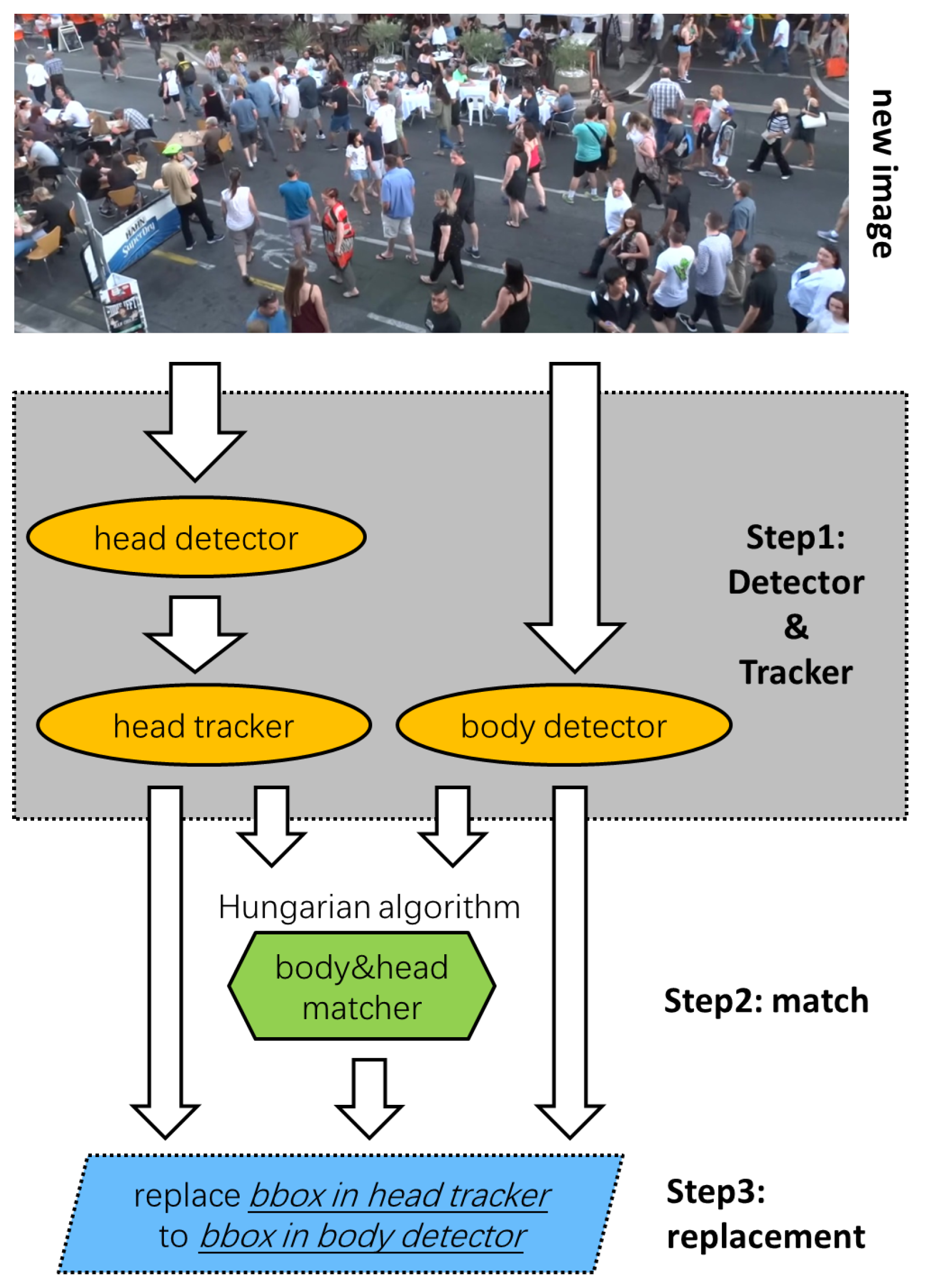
Our goal is to design a multiobject tracking system, named TraPeHat. An overview of the system is shown in Figure 2; our tacker is an online tracker. When our system receives a new frame, it works as follows.

Figure 2. The main architecture of our proposal, Tracking Pedestrians with Head Tracker (TraPeHat).

Step 1

Detect and track each pedestrian’s head in the current frame, as well as detect each pedestrian’s body.

Step 2

Integrate the information above. Specifically, pair the head bounding boxes with the full-body bounding boxes by determining whether they belong to the same pedestrian. If they do, we link these boxes to determine their relationship.

Step 3

According to the matching results in Step 2, the head bounding boxes in the head motion tracklets are replaced with the body bounding boxes, thus generating the final desired pedestrian body motion tracklets.

3.1. Detector and Tracker

During pedestrians’ movements, head tracklets (including head bounding boxes) and full-body bounding boxes are generated by using a head tracker and a body detector, respectively. The design of the head tracker follows the TDB paradigm which consists of a head detector and a head tracker. The whole-body detector was built based on Faster RCNN [12]. Next, we will describe how our head tracker and body detector work in detail.

3.1.1. Head Detector

In the head detection task, we need to generate the head bounding box for each pedestrian. The overall structure of our head detector is shown in Figure 3. It is an end-to-end two-stage detector, which consists of four functional modules.

Figure 3. The architecture of the head detector in our proposal.

Resnet50 with FPN. First, Resnet50 [53] was used as the backbone network, coupled with feature pyramid networks (FPNs) to extract multiscale features. In this scenario, FPNs downsampled gradually through a bottom-up operation under the effect of Resnet to obtain C1-C4, and then gradually upsampled M1-M4 through a top-down operation, and used the prediction heads to obtain multiple predictions with the same dimension and different sizes.

CSPM Model. Next, consider that there are many similarities between head detection and face detection tasks. For example, the shapes of the target bounding boxes are similar (approximately a square), and the differences between the targets’ appearance features are small. Therefore, both tasks have the difficulty of being easily confused among targets. For this, our method used a context-sensitive prediction module (SCPM) [54] derived from a face detection method named PyramidBox [55]. Inspired by Inception-ResNet [56], it took the predictions from the previous FPN module as input, and had multiple convolutions working in parallel, which were implemented by SSH [57] and DSSD [58]. SSH increased the receptive field of the model by configuring more and wider convolutional prediction models in parallel before other convolutional layers, which is the embodiment of Inception. DSSD added a residual block to each prediction module to increase the depth of the model, which was considered from the perspective of Resnet. The introduction of SSH and DSSD enhanced the model prediction module from the perspective of breadth and depth respectively, making it more capable of capturing wider and deeper feature information.

Transpose Convolutions. Then, we performed a transposed convolution [59] operation on the features of all pyramid levels. The convolution operation is essentially a downsampling operation. After the image passes through several convolution layers, a tensor is obtained, and its size is generally smaller than the size of the original image. Although the transposed convolution is essentially an upsampling operation, which could be considered the reverse operation of the convolution, it can be used to increase the size of the tensor and improve the spatial resolution of the feature mapping.

RPN and two heads. Finally, we used a region proposal network (RPN) [12] to generate target region proposals. RPN consists of four steps: generate anchors that may have targets, use Softmax classifier to identify the positive anchors, use bounding box regression to fine tune the selected positive anchors, and generate proposals through the proposal layer. Finally, the regression and classification heads are used to provide position offsets and target class confidence scores, respectively.

3.1.2. Head Tracker

Next, the outputs of head detector were input to the head tracker. The head tracker is an improved version of the particle filter [60]. The specific execution flow is as follows.

Initialization. The tracklets were initialized at the beginning of the input video, and the weight of each particle was equalled at the initialization. Each particle was represented by a four-dimensional state space, with the states of each target being modelled as $(x_c,y_c,w,h,\dot{x_c},\dot{y_c},\dot{w},\dot{h})$, where $(x_c,y_c,w,h)$ represent the center coordinates of x and y axis, widths, heights of the bounding boxes, and the dotted represent the next prediction for the bounding boxes. In addition, new tracklets were also initialized for the bounding boxes that cannot match any existing tracklets.

Predict and Update. For the subsequent video frame, a ROI pooling operation was performed on the feature maps of the targets of that frame. ROI pooling performed max pooling on inputs of nonuniform sizes to obtain feature maps of fixed sizes. This operation unified the sizes of the target feature maps without losing the local and shape information of the targets. Our particle filter refreshed the state information of particles through the prediction stage and update stage. In the particle prediction stage, the weight of each particle was set according to the foreground classification score of the classification head in Section 3.1.1. Then, we used the regression head in Section 3.1.1 to predict the position of each particle. The method of using the regression head to predict the positions of the particles is similar to that of [6], but the difference between them is that the bounding box regression operation was applied to the particles instead of the target tracklets in [6]. In the update stage of the particles, the weights of the particles were averaged to search the positions of the targets, and the corresponding formula is shown in (1). $S_t^k$ represents the predicted position of the kth tracklets in the tth frame, M is the number of particles, $p_t^{k,i}$ represents the position of ith particle associated with the kth tracklets in the tth frame; furthermore, $w_t^{k,i}$ represents the weight of $p_t^{k,i}$. We have

$$S_t^k = \frac{1}{M}\sum _{i = 1}^M{p}_t^{k,i}{w}_t^{k,i}.$$

(1)

Resample. The particle filter itself has degenerate problems [60], so we used resampling techniques to replace less important particles. When the weights of particles on the positions of the regression head were over the threshold ${\widehat{N}}_{eff}^k$, M particles of would be resampled. The threshold ${\widehat{N}}_{eff}^k$ is defined as shown in (2):

$${\widehat{N}}_{eff}^k = \frac{1}{{\sum }_{i = 1}^M{(w_t^{k,i})}^2}.$$

(2)

Cost Match. If the score of estimated state S of a tracklet was less than threshold $\mu$, the tracklet would be set to the inactive state. According to the constant velocity assumption (CVS) model, the next positions of these tracklets were estimated. If the positions of the new tracklets have a high similarity with the detection results, the tracking of these tracklets will be resumed. The similarity calculation method is shown in (3), where $\alpha$ and $\beta$ are parameters representing weights, $IoU$ represents the calculation of the IoU value between two bounding boxes, and $d^1$ represents the Bhattacharyya distance between the corresponding color histograms in the HSV space [61], $L_t^i$ and $N_t^j$ respectively represent the ith inactive and the jth newly initialized tracklets in the tth frame. Once the tracklets were reidentified, we reinitialized the particles around their new positions. We have

$$C = \alpha \ast IoU(L_t^i,N_t^j)+\beta \ast d^1(L_t^i,N_t^j).$$

(3)

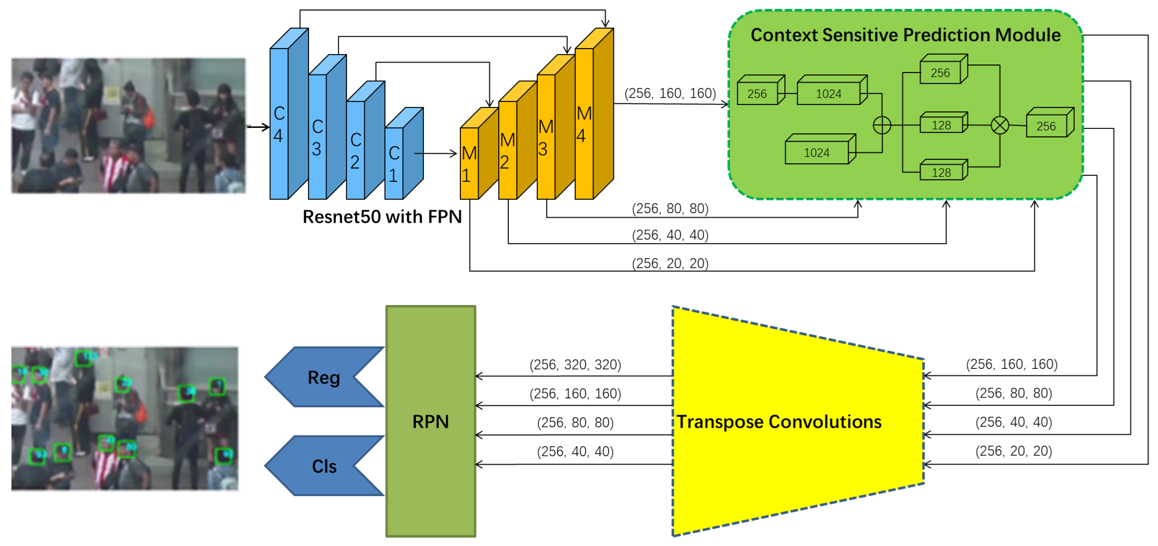
3.1.3. Body Detector

Several Fused GTs to One Proposal. The body detector needs to be competent in dense crowds, but the reality is the objects overlapped heavily in dense crowds, and it is difficult to deal with. Therefore, several ground-truth bounding boxes with high IoCs were fused together to one proposal in our method, each fused bounding box represented an independent object. The total objects after fusion are described as (4), where $b_i$ is the proposed box, $g_i$ is the ground-truth bounding box, and $\mathcal{G}$ represents the set of all ground-truth bounding boxes. $\theta$ is the threshold for IoU calculation. The fusing technique used here can effectively distinguish multiple overlapping objects. The detector obtains some sort of antiocclusion ability and achieve higher robustness. We have

$$G(b_i) = \{g_i \in \mathcal{G}|IoU(b_i,g_i) \ge \theta \}.$$

(4)

The overall structure of the whole-body detector is shown in Figure 4. We used the following method to perform pedestrians’ body detection.

Figure 4. The architecture of the body detector in our proposal. In this figure, on the far left side at Section (a) is the basic structure of Faster-RCNN. After the fully connected layer, each proposal predict multiple predicted bounding boxes ($bo{x}_A$ and $bo{x}_B$). After using EMD Loss to solve the losses between each predicted result and the ground truth bounding boxes, we used our patched NMS to suppress redundant bounding boxes. The refinement module was used to further refine the final results.

Predict Several Predictions for Each Proposal. There are multiple proposals for each picture, and the instance predictions of each proposal are represented by a set of predicted boxes as (5). Each predicted box is represented by $(c_i,l_i)$, where $c_i$ is the predicted category with confidence, and $l_i$ is the relative coordinates of the prediction, and K is a preset constant, indicating that each proposal can predict up to K predictions. We have

$$P(b_i) = \{(c_i^{(1)},l_i^{(1)}),(c_i^{(2)},l_i^{(2)}),...,(c_i^{(K)},l_i^{(K)})\}.$$

(5)

To calculate the differences, the Earth Mover’s Distance (EMD) method was introduced in our approach, which is essentially a vector similarity measurement that can be used to solve problems like Optimal Transport. Inspired by target detection algorithms such as [62,63,64], we used EMD Loss as the loss function for dense detection algorithm. The loss function is expressed as (6), where $\pi$ represents a sequence of real numbers, and the value of the $k^{th}$ item is the value k, $g_{{\pi }_k} \in G(b_i)$, where $g_{{\pi }_k}$ represents the kth ground-truth bounding boxes in the set of ground-truth, ${\mathcal{L}}_{cls}$ and ${\mathcal{L}}_{reg}$ represent the classification loss and the regression loss, respectively. We have

$$\mathcal{L}(b_i) = \underset{\pi \in \prod }{min}\sum _{k = 1}^K[{\mathcal{L}}_{cls}(c_i^{(k)},g_{{\pi }_k})+{\mathcal{L}}_{reg}(c_i^{(k)},g_{{\pi }_k})].$$

(6)

Patched NMS. The body detector adopt a patched version of Non-Maximum Suppression (NMS) when dealing with multiple bounding boxes with high overlaps. Specifically, when NMS suppresses one box for the other, it checks whether the two boxes belong to the same proposal by adding an additional test, and if so, skips the step. The patched NMS is used in conjunction with the fused examples, which has a significant effect in crowd detection.

Refinement Model. Each fused example contained several bounding boxes, which may lead to a higher risk of false positives. Hence a supplementary refinement module might be added, and the module is optional according to the quality of output results. The structure of the refinement module is shown in Figure 4b, which takes the predictions as input and combines them with the proposal boxes, to correct the wrong predictions due to the fusion.

3.2. Match

Bipartite Graph. Head bounding boxes and body bounding boxes obtained in Section 3.1.1 and Section 3.1.3 can be viewed as a bipartite graph. It is a special graph dividing vertices into two disjoint and independent sets. The vertices in these two sets are connected by edges, but not self-connected in one set. In our method, head bounding boxes and body bounding boxes respectively constitute the two sets of the bipartite graph, and the edges between two vertices were evaluated by the IoC calculation between the head bounding boxes and the the full-body bounding boxes.

IoC and Cost Matrix. The IoC reflects the extent to one bounding box covered one other bounding box, and is calculated in the ratio of the intersecting area between head and full-body bounding boxes to the area of the entire-body bounding box. As shown in (7), where $H_i$ and $B_j$ represent the ith head bounding box and the jth body bounding box. The IoC’s value is normalized to $[0,1]$. IoU is calculated in slightly different ways than IoC. The IoU is the ratio of the intersecting area to the area of both two bounding boxes. Figure 5 shows the definition and difference between IoC and IoU.

Figure 5. Definition and comparison of IoC and IoU.

We have

$$IoC(H_i,B_j) = \frac{|H_i\bigcup B_j|}{\left|B_j\right|}$$

(7)

$$\mathbf{CostMatrix} = \left(\begin{array}{ccc}IoC(H_1,B_1)& \dots & IoC(H_1,B_n)\\ ⋮& \ddots & ⋮\\ IoC(H_m,B_1)& \dots & IoC(H_m,B_n)\end{array}\right).$$

(8)

Hungarian algorithm. An IoC operation was performed between each head bounding box and each body bounding box in the current frame. The cost matrix is shown in (8), where m is the number of rows and n is the number of columns, i.e., m head boxes and n body boxes detected in the frame. Then the cost matrix was processed by the Hungarian algorithm. As an allocation algorithm, the Hungarian algorithm completed the matching of the targets’ (pedestrians) head bounding boxes and body bounding boxes as (9). We have

$$indice{s}_H,indice{s}_B = Hung(\mathbf{CostMatrix}).$$

(9)

3.3. Replacement

According to the matching of head bounding boxes and full-body bounding boxes in Section 3.2, we replace head bounding boxes in the head motion tracklets in Section 3.1.2 with body bounding boxes obtained in Section 3.1.3. For those body bounding boxes without matched head bounding boxes, and head bounding boxes without matched body bounding boxes, both types of boxes are discarded directly.

4. Experiment

4.1. General Settings

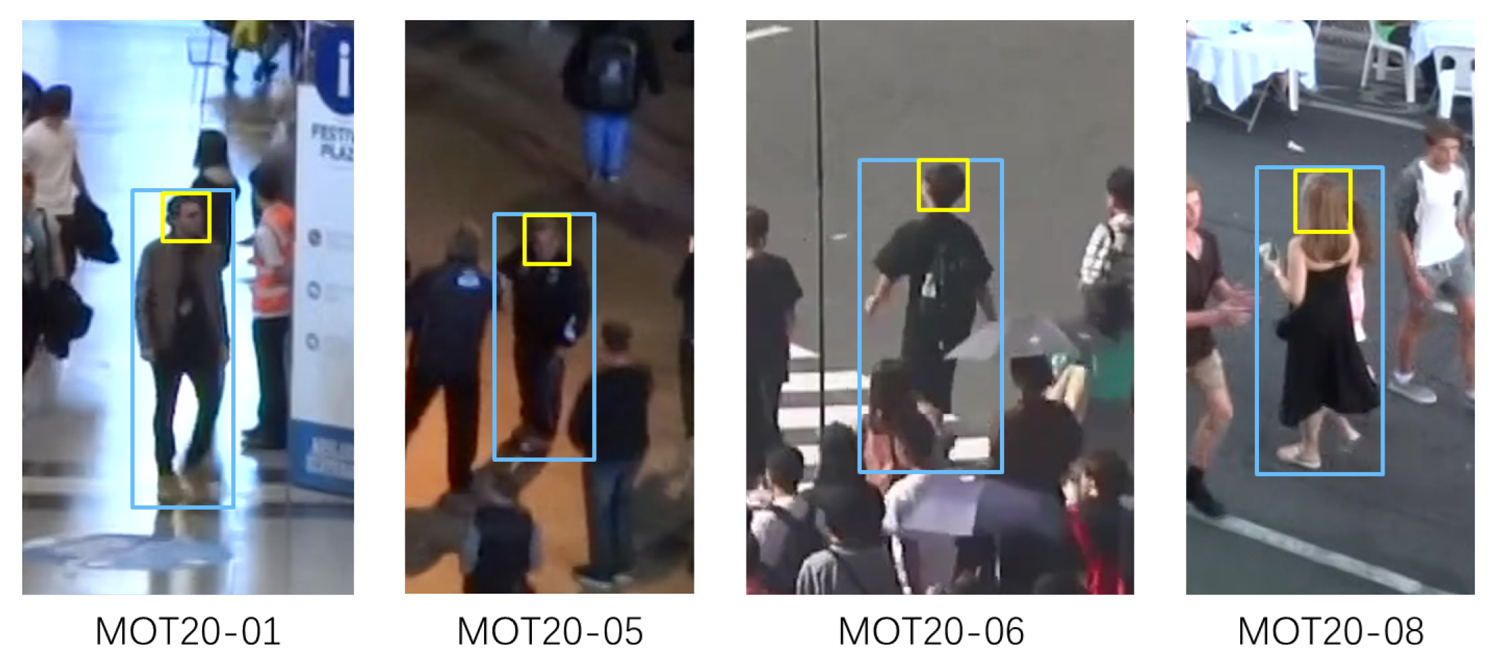
4.1.1. MOT20 Dataset

A large amount of experimental work was based on the MOT20 [8] dataset from the MOT Challenge [65]. MOT20 is a dataset concerning multiobject pedestrian tracking in dense crowds. The number of targets in MOT20 is overwhelming, and thus the targets in the dataset have abnormally serious occlusions, and the frequency of occlusions is relatively higher than other typical datasets. In MOT20, there are four video sequences lasting 357 s, a total of 8931 frames and 1,336,920 targets in the training set (average 149.7 targets per frame). There are four video sequences lasting 178 s in the training set, with 4479 frames and 765,465 targets in total, and 170.9 targets per frame on average [8]. Those raw videos were shot in many places during the day or night with dense pedestrians, including squares, stations, and streets. With indoor and outdoor, and day and night sequences, the rich scene elements can fully demonstrate the performance of the tracker.

The role of cross-validation is to reduce the negative impact of overfitting, and obtain as much effective information as possible from limited training data. Because the training set of MOT20 consists of four video sequences, we used fourfold cross-validation when training. In each fold, three videos were used for training and one video was used for testing, as shown in Figure 6.

Figure 6. Fourfold cross validation for training and testing.

4.1.2. Metrics

We used CLEAR [66] evaluation indicator that comprehensively consider FP, FN, and ID-Switch, which has a more common name called MOTA. The CLEAR reflects the tracking quality of tracker more comprehensively. However, the CLEAR ignores the ID characteristics of multiple targets, so we introduced IDF1 [67] additionally to make up for the lack of MOTA in this regard. In addition, HOTA [68] is an indicator that had just been proposed in recent years, which can reflect the effects of detection and matching in a balanced manner.

4.1.3. Some Details

When proceeding to the matching process in Section 3.2, we cut the body bounding boxes before performing the IoC operation. It was done by keeping only the top 35 pixels of the body bounding box and extending it upward by five pixels. In addition, we cut off the left and right 20% of the body bounding boxes, and only the middle 60% was kept, as shown in Figure 7. The reason for that is that the sizes of most of the head bounding boxes in the MOT20 dataset are generally less than 50 pixels, and the heads are generally located in the top and middle of the bodies, so the information on both sides and lower positions of the body bounding boxes is somewhat redundant. The matching accuracy was improved by eliminating redundant information of body bounding boxes.

Figure 7. The blue box in the figure is the original full body bounding box of the pedestrian, and the red bounding box is obtained after the above blue box is processed. The processing method has been shown in the figure: the shaded part of the blue box will be discarded, then expanded to generate the red box. Rather than the blue box, the red bounding box and the head bounding box are used for IoC operation.

The numbers mentioned above, or being named as a set of parameters, could be used to clip the head bounding boxes in the MOT20 dataset. In order to find a better set of parameters, we changed some parameters without changing other settings. Observe the performance of our method on the MOT20 dataset in Table 1. In Table 1, it can be found that {−20%, 5 pixels, 35 pixels} performed best, and we used this set of data in follow-up experiments. The differences among different sets of parameters are actually not very obverse. According to our statistics, the pedestrians’ heads in the MOT20 dataset occupy 25 ∗ 27 pixels on average. We also recommend using {−20%, five pixels, 35 pixels} as parameters in videos other than MOT20. If TraPeHat doesn’t perform well in other videos, randomly select a few frames, detect and calculate the average pixels occupied by pedestrian heads in these frames, then adjust parameters proportionally. Of course, we do not recommend adjusting a parameter of {−20%} because the variance of pedestrian head and body ratio is generally not too great.

Table 1. The impact on TraPeHat when using different parameters to cut the body bounding boxes. After considering the two most important tracking indicators, MOTA and HOTA, the group parameters of {−20%, five pixels, 35 pixels} performs best. (CutA: Ratios of pixels to cut off on left and right sides. Patch: Pixels patched to the top. CutB: Pixels kept at the bottom).

Cut A	Patch	CutB	MOTA↑	MOTP↑	IDF1↑	Idsw↓	HOTA↑
−20%	5px	35px	55.07	78.55	52.18	4342	41.11
−15%	5px	35px	55.04	78.54	52.16	4347	41.10
−25%	5px	35px	55.06	78.56	52.19	4354	41.11
−20%	0px	35px	54.99	78.56	52.15	4383	41.09
−20%	10px	35px	55.09	78.53	52.18	4318	41.11
−20%	5px	30px	54.81	78.55	52.04	4322	41.00
−20%	5px	40px	55.02	78.54	52.16	4348	41.08

4.2. Ablation Study on Match Methods

CTC. As we all know, a bounding box is a rectangle surrounded by four coils. In this section, we used CTC to denote the coordinates of the top center point of the head and body bounding boxes. Because the head is generally located at the top and middle of the body, the CTC of most pedestrians’ head bounding boxes should be very close to the CTC of their body bounding boxes, or even express the same pixel, as shown in Figure 8.

Figure 8. All subplots in this figure come from the MOT20 dataset, in which the positions of the heads are demarcated by the yellow bounding boxes and the positions of the bodies are demarcated by the blue bounding boxes. A general rule can be concluded from this figure: pedestrians’ head bounding boxes are more likely to be located in the middle and upper positions of their body bounding boxes.

LD and ED. To demonstrate the effectiveness of the IoC as an input weight for the association algorithm, we experimented with a variety of different weights. The location deviation (LD) of CTC coordinates of the two bounding boxes could be taken into account. LD maximizes confidences for head bounding boxes whereas those boxes are just above and centered on the body bounding boxes, as shown in (10), where $loc\_dev\_x(\ast )$ and $loc\_dev\_y(\ast )$ denote the location deviation between the body bounding boxes and the head bounding boxes from the x and y directions, respectively, and $\alpha$ and $\beta$ are hyperparameters. The Euclidean distance (ED) is a simple and crude measurement between two bounding boxes, as shown in (11), and this is used as the only calculation criterion for the degree of association. For LD and ED, the subsequent CostMatrix should also be changed, and the specific details will not be repeated. In (10) and (11), the CTC points of the head and body bounding boxes are denoted as $H_i$ and $B_j$ for the purposes of convenient expression and understanding. We have

$$LD(H_i,B_j) = \alpha \ast loc\_dev\_x(H_i,B_j)+\beta \ast loc\_dev\_y(H_i,B_j)$$

(10)

$$ED(H_i,B_j) = Eus\_dis(H_i,B_j).$$

(11)

The final results of the ablation study on match methods are shown in Table 2, from which it is not difficult to find that IoC achieves the best results. We speculate that the reason for this phenomenon is that IoC not only takes into account the distribution of the top center of the bounding box sets, but also reflects the extent to which the head bounding boxes are contained by the body bounding boxes, thus achieving the best results.

Table 2. After changing the method of measuring the similarities between heads and bodies in TraPeHat, the final performances of TraPeHat on the MOT20 dataset are shown. The directions of arrows indicate smaller or larger values are desired for the metric.

Method	MOTA↑	IDF1↑	HOTA↑
ED	37.89	34.46	34.52
LD	51.47	46.83	39.68
IoC(Ours)	55.07	52.18	41.12

4.3. Head Detection and Head Tracking Methods

SCUT-Head. SCUT-Head [9] is a large-scale head detection dataset, with 4405 images and 111,251 head labels in total. The dataset consists of two parts, Part A and Part B. Part A came from the surveillance cameras in certain university classrooms, and Part B was collected from the Internet, so the background of the images in this part is relatively wider. We compared our method with several common detectors on the SCUT-Head dataset, as shown in Table 3. The evaluation indicators like precision, recall and F1 scores were involved. It can be seen from Table 3 that our method is better than other general methods.

Table 3. The comparison between different head detection methods.

Method	Precision%	Recall%	F1
FasterRCNN [12]	87	80	0.83
RFCN+FRN [9]	91	84	0.87
SMD [69]	93	90	0.91
HSFA2Net [70]	94	92	0.93
TraPeHat(ours)	95	93	0.94

HT21. HT21 [7] is a large-scale pedestrian head tracking dataset in dense scenes. It consists of a training set and a testing set, with a total of 13,410 images and 2,102,385 head bounding boxes, and 6811 head motion trajectories, each frame contains 156.78 goals on average. SORT was mainly composed of Kalman filter and Hungarian algorithm. It detected bounding boxes and then tracked them, and it was a classic multiobject tracker. With the help of high-speed cameras, the IoU value between the same target in the previous and present two frames is considerable. Based on that idea, ref. [71] proposed the tracking algorithm V_IOU. Tracktor++ [6] cleverly used the function of bounding box regression of object detector to achieve target tracking. Comparing the above methods with our method in Table 4, we can see that our method has great advantages in various indicators.

Table 4. The comparison between different head tracking methods on HT21 dataset.

Method	MOTA↑	IDEucl↑	IDF1↑	MT↑	ML↓	ID Sw↓
SORT [1]	46.4	58.0	48.4	49	216	649
V_IOU [71]	53.4	34.3	35.4	80	182	1890
Tracktor++ [6]	58.9	31.8	38.5	125	117	3474
TraPeHat(ours)	63.6	60.3	57.1	146	93	892

4.4. Body Detection Methods

CrowdHuman. CrowdHuman [10] is a widely used dense pedestrian detection dataset, which consists of a training set, a testing set, and a validation set, with a total of 24,370 images, and an average of 23 targets per image. Pedestrian bodies in this dataset are often occluded by other pedestrians, so it is not an easy task to detect full bodies in this dataset. Comparing the full-body detection method used in our experiments with several common methods, the results are shown in Table 5. It can be seen that the main technical indicators of our method are in a leading position in this type of task.

Table 5. The comparison between different body detection methods on CrowdHuman dataset.

Method	AP/%	MR−2/%
Crowd Human Benchmark [10]	85.0	50.4
Adaptive NMS [72]	84.7	49.7
Soft-NMS [73]	88.2	42.9
PBM [74]	89.3	43.3
TraPeHat(ours)	90.7	41.4

4.5. Final Results on MOT20

For the performance of TraPeHat on the MOT20 training set, we ran and evaluated in our local devices. Because the MOT20 testing set does not expose its ground truth, our results were uploaded to the MOT Challenge website [65] for evaluation. The overall performance results of the training set and test set are shown in Table 6.

Table 6. The performance of our method TraPeHat on MOT20 testing set.

Video Sequence		MOTA↑	MOTP↑	HOTA↑	IDF1↑	MT↑	ML↓	FP↓	FN↓	ID Sw↓
	MOT20-04	70.71	80.85	54.27	67.15	45	3	4724	2556	39
	MOT20-06	68.94	81.05	47.38	55.76	162	8	4554	25,771	364
Testing Set	MOT20-07	53.05	76.98	40.48	55.19	117	147	5127	58,201	564
	MOT20-08	52.25	78.45	39.18	49.37	248	202	7166	126,087	3375
	OVERALL	55.07	78.55	41.12	52.18	572	360	21,571	212,615	4342

We compared TraPeHat with some other trackers on the MOT20 dataset, the running results of which were from the MOT Challenge website [65], as shown in Table 7, from which we can see that our algorithm achieved a comparable effect. Our method is superior to the other methods in Table 7 in most of the multiobject tracking indicators. From this, we can learn that TraPeHat achieved higher MOTA, HOTA, and IDF1 scores, and the scores of FP, FN were lower. However, the ML and ID-Switch indicators of FlowTracker were slightly better than TraPeHat. We speculate that the reason for this phenomenon is as follows. FlowTracker used optical flow to realize multiobject tracking, and the principle of multiobject tracker based on optical flow method is that the appearance features of the same pedestrian do not change significantly in two adjacent frames. TraPeHat, on the other hand, did not use target appearance information in the matching stage. Therefore, FlowTracker used more comprehensive appearance information than TraPeHat, and this also gives FlowTracker an advantage when dealing with continuous targets and ID Switch. But TraPeHat integrates head tracking which enforced the overall tracking performance on MOTA, HOTA, and so on. It is worth mentioning that we did not use any deep learning tricks to improve the accuracy in the whole experiments.

Table 7. We compared our online multiobject tracker TraPeHat with other modern tracking methods. As the most valuable evaluation indicator in the field of multiobject tracking, the overall pros and cons of the algorithm are sorted from top to bottom according to the MOTA value. We can see that TraPeHat has achieved competitive results.

Algorithm	MOTA↑	HOTA↑	IDF1↑	MT↑	ML↓	FP↓	FN↓	ID Sw↓
OVBT17 [75]	40.00	30.50	37.80	141	374	23,368	282,949	4210
SORT20 [1]	42.70	36.10	45.10	208	326	27,521	264,694	4470
GMPHD_Rd20 [76]	44.70	35.60	43.50	293	274	42,778	236,116	7492
IOU_KMM [77]	46.50	40.40	49.40	371	371	57,517	214,777	4509
FlowTracker [78]	46.70	35.60	42.40	345	249	54,732	217,371	3352
BBT [79]	46.80	35.80	42.20	312	289	35,014	236,176	3880
SFS [80]	50.80	32.70	41.10	341	251	50,139	220,932	3503
TraPeHat(ours)	55.10	41.10	52.20	572	360	21,571	212,615	4342

5. Conclusions

Building on the work of Sundararaman et al. [7], by using pedestrian head tracking, we extended the tracked objects from the pedestrians’ heads to the pedestrians’ whole bodies. In order to achieve the above goals, we proposed a bounding box similarity measurement method named IoC, which can effectively complete the matching work of the same target’s head bounding box and body bounding box. A series of related experiments demonstrated the effectiveness of this method. We hope that this method can effectively reduce the inconvenience caused by severe occlusions for pedestrian tracking tasks in dense environments, and provide references for subsequent head tracking tasks.

References

1. Bewley, A.; Ge, Z.; Ott, L.; Ramos, F.; Upcroft, B. Simple online and realtime tracking. In Proceedings of the 2016 IEEE International Conference on Image Processing (ICIP), Phoenix, AZ, USA, 25–28 September 2016; pp. 3464–3468. [Google Scholar] [CrossRef]
2. Wojke, N.; Bewley, A. Deep Cosine Metric Learning for Person Re-identification. In Proceedings of the 2018 IEEE Winter Conference on Applications of Computer Vision (WACV), Lake Tahoe, NV, USA, 12–15 March 2018; pp. 748–756. [Google Scholar] [CrossRef]
3. Zhang, Y.; Sun, P.; Jiang, Y.; Yu, D.; Weng, F.; Yuan, Z.; Luo, P.; Liu, W.; Wang, X. ByteTrack: Multiobject Tracking by Associating Every Detection Box. arXiv 2021, arXiv:2110.06864. [Google Scholar] [CrossRef]
4. Zhang, Y.; Wang, C.; Wang, X.; Zeng, W.; Liu, W. FairMOT: On the Fairness of Detection and Re-Identification in Multiple Object Tracking. Int. J. Comput. Vis. 2021, 129, 3069–3087. [Google Scholar] [CrossRef]
5. Chen, L.; Ai, H.; Zhuang, Z.; Shang, C. Real-Time Multiple People Tracking with Deeply Learned Candidate Selection and Person Re-Identification. In Proceedings of the 2018 IEEE International Conference on Multimedia and Expo (ICME), San Diego, CA, USA, 23–27 July 2018; pp. 1–6. [Google Scholar] [CrossRef]
6. Bergmann, P.; Meinhardt, T.; Leal-Taixe, L. Tracking Without Bells and Whistles. In Proceedings of the 2019 IEEE/CVF International Conference on Computer Vision (ICCV), Seoul, Republic of Korea, 27 October–2 November 2019. [Google Scholar] [CrossRef]
7. Sundararaman, R.; De Almeida Braga, C.; Marchand, E.; Pettré, J. Tracking Pedestrian Heads in Dense Crowd. In Proceedings of the 2021 IEEE/CVF Conference on Computer Vision and Pattern Recognition (CVPR), Nashville, TN, USA, 20–25 June 2021; pp. 3864–3874. [Google Scholar] [CrossRef]
8. Dendorfer, P.; Rezatofighi, H.; Milan, A.; Shi, J.; Cremers, D.; Reid, I.; Roth, S.; Schindler, K.; Leal-Taixé, L. MOT20: A benchmark for multi object tracking in crowded scenes. arXiv 2020, arXiv:2003.09003. [Google Scholar] [CrossRef]
9. Peng, D.; Sun, Z.; Chen, Z.; Cai, Z.; Xie, L.; Jin, L. Detecting Heads using Feature Refine Net and Cascaded Multi-scale Architecture. arXiv 2018, arXiv:1803.09256. [Google Scholar]
10. Shao, S.; Zhao, Z.; Li, B.; Xiao, T.; Yu, G.; Zhang, X.; Sun, J. CrowdHuman: A Benchmark for Detecting Human in a Crowd. arXiv 2018, arXiv:1805.00123 2018. [Google Scholar] [CrossRef]
11. Krizhevsky, A.; Sutskever, I.; Hinton, G.E. ImageNet Classification with Deep Convolutional Neural Networks. Commun. ACM 2017, 60, 84–90. [Google Scholar] [CrossRef]
12. Ren, S.; He, K.; Girshick, R.; Sun, J. Faster R-CNN: Towards Real-Time Object Detection with Region Proposal Networks. IEEE Trans. Pattern Anal. Mach. Intell. 2017, 39, 1137–1149. [Google Scholar] [CrossRef]
13. Redmon, J.; Farhadi, A. YOLOv3: An Incremental Improvement. arXiv 2018, arXiv:1804.02767. [Google Scholar]
14. Lin, T.Y.; Goyal, P.; Girshick, R.; He, K.; Dollár, P. Focal Loss for Dense Object Detection. In Proceedings of the 2017 IEEE International Conference on Computer Vision (ICCV), Venice, Italy, 22–29 October 2017; pp. 2999–3007. [Google Scholar] [CrossRef]
15. Sun, P.; Jiang, Y.; Xie, E.; Shao, W.; Yuan, Z.; Wang, C.; Luo, P. What Makes for End-to-End Object Detection? In Proceedings of the 38th International Conference on Machine Learning, Virtual Event, 18–24 July 2021; Meila, M., Zhang, T., Eds.; PMLR: New York, NY, USA, 2021; Volume 139, pp. 9934–9944. [Google Scholar]
16. Fu, J.; Zong, L.; Li, Y.; Li, K.; Yang, B.; Liu, X. Model Adaption Object Detection System for Robot. In Proceedings of the 2020 39th Chinese Control Conference (CCC), Shenyang, China, 27–29 July 2020; pp. 3659–3664. [Google Scholar] [CrossRef]
17. Cai, Z.; Vasconcelos, N. Cascade R-CNN: Delving Into High Quality Object Detection. In Proceedings of the 2018 IEEE/CVF Conference on Computer Vision and Pattern Recognition, Salt Lake City, UT, USA, 18–22 June 2018; pp. 6154–6162. [Google Scholar] [CrossRef]
18. Sun, P.; Zhang, R.; Jiang, Y.; Kong, T.; Xu, C.; Zhan, W.; Tomizuka, M.; Li, L.; Yuan, Z.; Wang, C.; et al. Sparse R-CNN: End-to-End Object Detection with Learnable Proposals. In Proceedings of the 2021 IEEE/CVF Conference on Computer Vision and Pattern Recognition (CVPR), Nashville, TN, USA, 20–25 June 2021; pp. 14449–14458. [Google Scholar] [CrossRef]
19. He, K.; Gkioxari, G.; Dollár, P.; Girshick, R. Mask R-CNN. In Proceedings of the 2017 IEEE International Conference on Computer Vision (ICCV), Venice, Italy, 22–29 October 2017; pp. 2980–2988. [Google Scholar] [CrossRef]
20. Lin, T.Y.; Dollár, P.; Girshick, R.; He, K.; Hariharan, B.; Belongie, S. Feature Pyramid Networks for Object Detection. In Proceedings of the 2017 IEEE Conference on Computer Vision and Pattern Recognition (CVPR), Honolulu, HI, USA, 21–26 July 2017; pp. 936–944. [Google Scholar] [CrossRef]
21. Long, J.; Shelhamer, E.; Darrell, T. Fully convolutional networks for semantic segmentation. In Proceedings of the 2015 IEEE Conference on Computer Vision and Pattern Recognition (CVPR), Boston, MA, USA, 7–12 June 2015; pp. 3431–3440. [Google Scholar] [CrossRef]
22. Lu, Z.; Rathod, V.; Votel, R.; Huang, J. RetinaTrack: Online Single Stage Joint Detection and Tracking. In Proceedings of the 2020 IEEE/CVF Conference on Computer Vision and Pattern Recognition (CVPR), Seattle, WA, USA, 13–19 June 2020; pp. 14656–14666. [Google Scholar] [CrossRef]
23. Peng, J.; Wang, C.; Wan, F.; Wu, Y.; Wang, Y.; Tai, Y.; Wang, C.; Li, J.; Huang, F.; Fu, Y. Chained-Tracker: Chaining Paired Attentive Regression Results for End-to-End Joint Multiple-Object Detection and Tracking. arXiv 2020, arXiv:2007.14557. [Google Scholar] [CrossRef]
24. Bochkovskiy, A.; Wang, C.Y.; Liao, H.Y.M. YOLOv4: Optimal Speed and Accuracy of Object Detection. arXiv 2020, arXiv:2004.10934. [Google Scholar]
25. Liang, C.; Zhang, Z.; Zhou, X.; Li, B.; Zhu, S.; Hu, W. Rethinking the Competition Between Detection and ReID in Multiobject Tracking. IEEE Trans. Image Process. 2022, 31, 3182–3196. [Google Scholar] [CrossRef] [PubMed]
26. Liang, C.; Zhang, Z.; Zhou, X.; Li, B.; Hu, W. One More Check: Making “Fake Background” Be Tracked Again. arXiv 2021, arXiv:2104.09441. [Google Scholar] [CrossRef]
27. Chu, P.; Wang, J.; You, Q.; Ling, H.; Liu, Z. TransMOT: Spatial-Temporal Graph Transformer for Multiple Object Tracking. arXiv 2021, arXiv:2104.00194. [Google Scholar]
28. Ge, Z.; Liu, S.; Wang, F.; Li, Z.; Sun, J. YOLOX: Exceeding YOLO Series in 2021. arXiv 2021, arXiv:2107.08430. [Google Scholar]
29. Zhou, X.; Wang, D.; Krähenbühl, P. Objects as Points. arXiv 2019, arXiv:1904.07850. [Google Scholar] [CrossRef]
30. Wu, J.; Cao, J.; Song, L.; Wang, Y.; Yang, M.; Yuan, J. Track to Detect and Segment: An Online multiobject Tracker. In Proceedings of the 2021 IEEE/CVF Conference on Computer Vision and Pattern Recognition (CVPR), Nashville, TN, USA, 20–25 June 2021; pp. 12347–12356. [Google Scholar] [CrossRef]
31. Zheng, L.; Tang, M.; Chen, Y.; Zhu, G.; Wang, J.; Lu, H. Improving Multiple Object Tracking with Single Object Tracking. In Proceedings of the 2021 IEEE/CVF Conference on Computer Vision and Pattern Recognition (CVPR), Nashville, TN, USA, 20–25 June 2021; pp. 2453–2462. [Google Scholar] [CrossRef]
32. Wang, Y.; Kitani, K.; Weng, X. Joint Object Detection and multiobject Tracking with Graph Neural Networks. In Proceedings of the 2021 IEEE International Conference on Robotics and Automation (ICRA), Xi’an, China, 30 May–5 June 2021; pp. 13708–13715. [Google Scholar] [CrossRef]
33. Tokmakov, P.; Li, J.; Burgard, W.; Gaidon, A. Learning to Track with Object Permanence. In Proceedings of the 2021 IEEE/CVF International Conference on Computer Vision (ICCV), Montreal, QC, Canada, 10–17 October 2021; pp. 10840–10849. [Google Scholar] [CrossRef]
34. Wang, Q.; Zheng, Y.; Pan, P.; Xu, Y. Multiple Object Tracking with Correlation Learning. In Proceedings of the 2021 IEEE/CVF Conference on Computer Vision and Pattern Recognition (CVPR), Nashville, TN, USA, 20–25 June 2021; pp. 3875–3885. [Google Scholar] [CrossRef]
35. Wojke, N.; Bewley, A.; Paulus, D. Simple Online and Realtime Tracking with a Deep Association Metric. In Proceedings of the 2017 IEEE International Conference on Image Processing (ICIP), Beijing, China, 17–20 September 2017; pp. 3645–3649. [Google Scholar] [CrossRef]
36. Basar, T. A New Approach to Linear Filtering and Prediction Problems. In Control Theory: Twenty-Five Seminal Papers (1932–1981); Wiley-IEEE Press: Hoboken, NJ, USA, 2001; pp. 167–179. [Google Scholar] [CrossRef]
37. Khan, J.; Fayaz, M.; Hussain, A.; Khalid, S.; Mashwani, W.; Gwak, J. An Improved Alpha Beta Filter using A Deep Extreme Learning Machine. IEEE Access 2021, PP, 1. [Google Scholar] [CrossRef]
38. Khan, J.; Kim, K. A Performance Evaluation of the Alpha-Beta (α-β) Filter Algorithm with Different Learning Models: DBN, DELM, and SVM. Appl. Sci. 2022, 12, 9429. [Google Scholar] [CrossRef]
39. Kuhn, H.W. The Hungarian Method for the Assignment Problem. In 50 Years of Integer Programming 1958–2008: From the Early Years to the State-of-the-Art; Jünger, M., Liebling, T.M., Naddef, D., Nemhauser, G.L., Pulleyblank, W.R., Reinelt, G., Rinaldi, G., Wolsey, L.A., Eds.; Springer: Berlin/Heidelberg, Germany, 2010; pp. 29–47. [Google Scholar] [CrossRef]
40. Wang, Z.; Zheng, L.; Liu, Y.; Wang, S. Towards Real-Time multiobject Tracking. arXiv 2020, arXiv:1909.12605. [Google Scholar]
41. Zhang, Y.; Wang, C.; Wang, X.; Liu, W.; Zeng, W. VoxelTrack: Multi-Person 3D Human Pose Estimation and Tracking in the Wild. IEEE Trans. Pattern Anal. Mach. Intell. 2022. [Google Scholar] [CrossRef]
42. Pang, J.; Qiu, L.; Li, X.; Chen, H.; Li, Q.; Darrell, T.; Yu, F. Quasi-Dense Similarity Learning for Multiple Object Tracking. In Proceedings of the 2021 IEEE/CVF Conference on Computer Vision and Pattern Recognition (CVPR), Nashville, TN, USA, 20–25 June 2021; pp. 164–173. [Google Scholar] [CrossRef]
43. Vaswani, A.; Shazeer, N.; Parmar, N.; Uszkoreit, J.; Jones, L.; Gomez, A.N.; Kaiser, L.; Polosukhin, I. Attention is All You Need. In Proceedings of the 31st International Conference on Neural Information Processing Systems, NIPS’17, Long Beach, CA, USA, 4–9 December 2017; Curran Associates Inc.: Red Hook, NY, USA, 2017; pp. 6000–6010. [Google Scholar]
44. Wang, W.; Xie, E.; Li, X.; Fan, D.P.; Song, K.; Liang, D.; Lu, T.; Luo, P.; Shao, L. Pyramid Vision Transformer: A Versatile Backbone for Dense Prediction without Convolutions. arXiv 2021, arXiv:2102.12122. [Google Scholar] [CrossRef]
45. Liu, Z.; Lin, Y.; Cao, Y.; Hu, H.; Wei, Y.; Zhang, Z.; Lin, S.; Guo, B. Swin Transformer: Hierarchical Vision Transformer using Shifted Windows. In Proceedings of the 2021 IEEE/CVF International Conference on Computer Vision (ICCV), Montreal, QC, Canada, 10–17 October 2021; pp. 9992–10002. [Google Scholar] [CrossRef]
46. Carion, N.; Massa, F.; Synnaeve, G.; Usunier, N.; Kirillov, A.; Zagoruyko, S. End-to-End Object Detection with Transformers. arXiv 2020, arXiv:2005.12872. [Google Scholar] [CrossRef]
47. Dosovitskiy, A.; Beyer, L.; Kolesnikov, A.; Weissenborn, D.; Zhai, X.; Unterthiner, T.; Dehghani, M.; Minderer, M.; Heigold, G.; Gelly, S.; et al. An Image is Worth 16x16 Words: Transformers for Image Recognition at Scale. arXiv 2020, arXiv:2010.11929. [Google Scholar] [CrossRef]
48. Chen, M.; Radford, A.; Wu, J.; Jun, H.; Dhariwal, P.; Luan, D.; Sutskever, I. Generative Pretraining From Pixels. In Proceedings of the ICML, Online, 13–18 July 2020. [Google Scholar]
49. Liu, R.; Yuan, Z.; Liu, T.; Xiong, Z. End-to-end Lane Shape Prediction with Transformers. In Proceedings of the 2021 IEEE Winter Conference on Applications of Computer Vision (WACV), Waikoloa, HI, USA, 5–8 January 2021; pp. 3693–3701. [Google Scholar] [CrossRef]
50. Sun, P.; Cao, J.; Jiang, Y.; Zhang, R.; Xie, E.; Yuan, Z.; Wang, C.; Luo, P. TransTrack: Multiple-Object Tracking with Transformer. arXiv 2020, arXiv:2012.15460. [Google Scholar]
51. Meinhardt, T.; Kirillov, A.; Leal-Taixe, L.; Feichtenhofer, C. TrackFormer: Multiobject Tracking with Transformers. In Proceedings of the IEEE Conference on Computer Vision and Pattern Recognition (CVPR), New Orleans, LA, USA, 18–24 June 2022. [Google Scholar]
52. Xu, Y.; Ban, Y.; Delorme, G.; Gan, C.; Rus, D.; Alameda-Pineda, X. TransCenter: Transformers with Dense Queries for Multiple-Object Tracking. arXiv 2021, arXiv:2103.15145. [Google Scholar]
53. He, K.; Zhang, X.; Ren, S.; Sun, J. Deep Residual Learning for Image Recognition. In Proceedings of the 2016 IEEE Conference on Computer Vision and Pattern Recognition (CVPR), Las Vegas, NA, USA, 27–30 June 2016; pp. 770–778. [Google Scholar] [CrossRef]
54. Tang, X.; Du, D.K.; He, Z.; Liu, J. PyramidBox: A Context-Assisted Single Shot Face Detector. In Proceedings of the Computer Vision—ECCV 2018, Munich, Germany, 8–14 September 2018; Ferrari, V., Hebert, M., Sminchisescu, C., Weiss, Y., Eds.; Springer International Publishing: Cham, Switzerland, 2018; pp. 812–828. [Google Scholar]
55. Tang, X.; Du, D.K.; He, Z.; Liu, J. PyramidBox: A Context-assisted Single Shot Face Detector. arXiv 2018, arXiv:1803.07737. [Google Scholar] [CrossRef]
56. Szegedy, C.; Ioffe, S.; Vanhoucke, V.; Alemi, A. Inception-v4, Inception-ResNet and the Impact of Residual Connections on Learning. arXiv 2016, arXiv:1602.07261. [Google Scholar] [CrossRef]
57. Najibi, M.; Samangouei, P.; Chellappa, R.; Davis, L.S. SSH: Single Stage Headless Face Detector. In Proceedings of the 2017 IEEE International Conference on Computer Vision (ICCV), Venice, Italy, 22–29 October 2017; pp. 4885–4894. [Google Scholar] [CrossRef]
58. Fu, C.Y.; Liu, W.; Ranga, A.; Tyagi, A.; Berg, A.C. DSSD: Deconvolutional Single Shot Detector. arXiv 2017, arXiv:1701.06659. [Google Scholar] [CrossRef]
59. Dumoulin, V.; Visin, F. A guide to convolution arithmetic for deep learning. arXiv 2016, arXiv:1603.07285. [Google Scholar] [CrossRef]
60. Arulampalam, M.; Maskell, S.; Gordon, N.; Clapp, T. A tutorial on particle filters for online nonlinear/non-Gaussian Bayesian tracking. IEEE Trans. Signal Process. 2002, 50, 174–188. [Google Scholar] [CrossRef]
61. Ding, D.; Jiang, Z.; Liu, C. Object tracking algorithm based on particle filter with color and texture feature. In Proceedings of the 2016 35th Chinese Control Conference (CCC), Chengdu, China, 27–29 July 2016; pp. 4031–4036. [Google Scholar] [CrossRef]
62. Szegedy, C.; Reed, S.; Erhan, D.; Anguelov, D.; Ioffe, S. Scalable, High-Quality Object Detection. arXiv 2014, arXiv:1412.1441. [Google Scholar] [CrossRef]
63. Stewart, R.; Andriluka, M. End-to-end people detection in crowded scenes. arXiv 2015, arXiv:1506.04878. [Google Scholar] [CrossRef]
64. Erhan, D.; Szegedy, C.; Toshev, A.; Anguelov, D. Scalable Object Detection Using Deep Neural Networks. In Proceedings of the 2014 IEEE Conference on Computer Vision and Pattern Recognition, Columbus, OH, USA, 23–28 June 2014; pp. 2155–2162. [Google Scholar] [CrossRef]
65. MOT Challenge. Available online: https://motchallenge.net/ (accessed on 23 December 2022).
66. Bernardin, K.; Stiefelhagen, R. Evaluating Multiple Object Tracking Performance: The CLEAR MOT Metrics. J. Image Video Process. 2008, 2008, 246309. [Google Scholar] [CrossRef]
67. Rezatofighi, H.; Tsoi, N.; Gwak, J.; Sadeghian, A.; Reid, I.; Savarese, S. Generalized Intersection Over Union: A Metric and a Loss for Bounding Box Regression. In Proceedings of the 2019 IEEE/CVF Conference on Computer Vision and Pattern Recognition (CVPR), Long Beach, CA, USA, 15–20 June 2019; pp. 658–666. [Google Scholar] [CrossRef]
68. Luiten, J.; Osep, A.; Dendorfer, P.; Torr, P.; Geiger, A.; Leal-Taixé, L.; Leibe, B. HOTA: A Higher Order Metric for Evaluating multiobject Tracking. Int. J. Comput. Vis. 2021, 129, 1–31. [Google Scholar] [CrossRef] [PubMed]
69. Sun, Z.; Peng, D.; Cai, Z.; Chen, Z.; Jin, L. Scale Mapping and Dynamic Re-Detecting in Dense Head Detection. In Proceedings of the 2018 25th IEEE International Conference on Image Processing (ICIP), Athens, Greece, 7–10 October 2018; pp. 1902–1906. [Google Scholar] [CrossRef]
70. Shen, W.; Qin, P.; Zeng, J. An Indoor Crowd Detection Network Framework Based on Feature Aggregation Module and Hybrid Attention Selection Module. In Proceedings of the 2019 IEEE/CVF International Conference on Computer Vision Workshop (ICCVW), Seoul, Republic of Korea, 27–28 October 2019; pp. 82–90. [Google Scholar]
71. Bochinski, E.; Senst, T.; Sikora, T. Extending IOU Based multiobject Tracking by Visual Information. In Proceedings of the 2018 15th IEEE International Conference on Advanced Video and Signal Based Surveillance (AVSS), Auckland, New Zealand, 27–30 November 2018; pp. 1–6. [Google Scholar] [CrossRef]
72. Liu, S.; Huang, D.; Wang, Y. Adaptive NMS: Refining Pedestrian Detection in a Crowd. arXiv 2019, arXiv:1904.03629. [Google Scholar] [CrossRef]
73. Bodla, N.; Singh, B.; Chellappa, R.; Davis, L.S. Soft-NMS – Improving Object Detection With One Line of Code. arXiv 2017, arXiv:1704.04503. [Google Scholar] [CrossRef]
74. Huang, X.; Ge, Z.; Jie, Z.; Yoshie, O. NMS by Representative Region: Towards Crowded Pedestrian Detection by Proposal Pairing. arXiv 2020, arXiv:1704.04503. [Google Scholar] [CrossRef]
75. Ban, Y.; Ba, S.; Alameda-Pineda, X.; Horaud, R. Tracking Multiple Persons Based on a Variational Bayesian Model. In European Conference on Computer Vision; Springer: Cham, Switzerland, 2016; Volume 9914, pp. 52–67. [Google Scholar] [CrossRef]
76. Baisa, N.L. Occlusion-robust online multiobject visual tracking using a GM-PHD filter with CNN-based re-identification. J. Vis. Commun. Image Represent. 2021, 80, 103279. [Google Scholar] [CrossRef]
77. Urbann, O.; Bredtmann, O.; Otten, M.; Richter, J.P.; Bauer, T.; Zibriczky, D. Online and Real-Time Tracking in a Surveillance Scenario. arXiv 2021, arXiv:2106.01153. [Google Scholar]
78. Nishimura, H.; Komorita, S.; Kawanishi, Y.; Murase, H. SDOF-Tracker: Fast and Accurate Multiple Human Tracking by Skipped-Detection and Optical-Flow. arXiv 2021, arXiv:2106.14259. [Google Scholar] [CrossRef]
79. Elias, P.; Macko, M.; Sedmidubsky, J.; Zezula, P. Tracking subjects and detecting relationships in crowded city videos. Multimed. Tools Appl. 2022, 23–30. [Google Scholar] [CrossRef]
80. Online multiobject Tracking Based on Salient Feature Selection in Crowded Scenes. Available online: https://motchallenge.net/method/MOT=2947&chl=13 (accessed on 23 December 2022).
Disclaimer/Publisher’s Note: The statements, opinions and data contained in all publications are solely those of the individual author(s) and contributor(s) and not of MDPI and/or the editor(s). MDPI and/or the editor(s) disclaim responsibility for any injury to people or property resulting from any ideas, methods, instructions or products referred to in the content.
Article Metrics
Citations
Article Access Statistics
Multiple requests from the same IP address are counted as one view.