Energy Cost Minimization with Hybrid Energy Storage System Using Optimization Algorithm

Featured Application

Energy storage systems, microgrids.

Abstract

The purpose of this study is to develop an effective control method for a hybrid energy storage system composed by a flow battery for daily energy balancing and a lithium-ion battery to provide peak power. It is assumed that the system operates behind the meter, the goal is to minimize the energy cost in the presence of a PV installation (as an example of a local renewable source) and energy prices are determined by 3-zone tariffs. The article presents the application of an optimization method to schedule the operation of each battery in the system. The authors have defined an optimization method aimed at minimizing the total cost of the system, taking into account energy costs and batteries depreciation. The techno-economical model of the system, including battery degradation, is constructed and the cost optimization methods are implemented in Python. The results are validated with real energy and price profiles and compared with conventional control strategies. The advantages of optimization in terms of energy cost are discussed. The experiment shows that not only is a hybrid energy system successful in lowering the total operation cost and in increasing self-consumption but also that the implemented methods have slightly different properties, benefits and issues.

1. Introduction

Large scale deployment of energy storage systems (ESS) is seen as a cost-effective solution for deep decarbonization of electric power systems, which also allows the system stability in the presence of intermittent renewable energy sources (RES) to be maintained [1]. ESS are also seen as part of the solution to reduce the reliance on external fossil fuel imports and high electricity prices [2]. Among available technologies, pumped hydro is still leading; however, grid-scale battery storage is gaining momentum with lithium-ion technology leading and flow batteries emerging [3]. In [4], the overview of technologies, optimization objectives and approaches regarding battery energy storage systems are presented.

Each battery technology is suited for different applications, ranging from short term power system stabilization requiring high power [5] to energy balancing on a daily basis that requires high capacity [6]. The most popular goal of using ESS is the reduction of the operation costs and the maximization of the self-consumption from RES. The profitability aspects are key for the practical popularization of energy storage. An ESS enhances the possibilities of the system by introducing the possibility of shifting part of the energy usage from the moments when cheap or surplus energy is available to the times when it is most needed and/or most costly. The economic outcome is one of the most popular optimization goals realized by a number of methods using classic, e.g., mixed-integer linear programming [7] and heuristic methods, e.g., deep reinforcement learning [8], genetic algorithm and particle swarm optimization [9].

Energy storage is usually just an element of a more complex system that manages the installations and the whole microgrid. Such systems need to be governed by so called energy management systems (EMS), which have been developed for a long time in various configurations. The key to battery functionality and long life depends largely on the battery management system (BMS) and the EMS [9]. Many such models have been developed; some focus on a very detailed model that includes temperatures, voltages, currents and state of charge, e.g., [10], while others use less detailed models but consider the long-term behavior of the system [11].

Basic concepts and different topologies of EMS are presented in [12]; the review of the different approaches can be found in [13,14]. In [15], an EMS, including battery management, which was tested in a real-life environment, is presented.

Hybrid energy storage systems (HESS), consisting of at least two battery types with complementary characteristics, are seen as a comprehensive solution in many applications [16]. Specifically, stationary microgrids seem to benefit from HESS integration [17]; their role may include energy balancing [18], power quality improvement [19] and off-grid operation [20]. Although most of the articles that focus on the energy management of HESS refer to electric vehicles and battery/supercapacitor combination, stationary applications are less explored.

In the review [21], the general classification of energy management systems that are focused on hybrid energy storages is presented. The types of management systems are divided by the objectives and by types, with two general categories: a classical approach and an intelligent approach. There are a few publications regarding EMS that consider hybrid energy storage. In [22], the application of a hybrid storage, consisting of a flow battery and a lithium battery, were simulated for a setup with off-grid renewable power. Ref. [23] shows the advantages of heterogeneous energy storage systems but also explains the possible problems with the implementation of EMS in such a setup, especially when the characteristics of the batteries are substantially different.

The challenge in developing a HESS is to create a more optimal environment for batteries of different technologies in order to maximize their lifetime and the benefits resulting from their operation. We approach this by enclosing the different battery technologies in a single system, a sort of energy storage black box from outside, which automatically creates the best possible environment and usage patterns for the contained technologies.

In order to make the hybrid battery work, a modular EMS is created that consists of two parts: an optimizer that uses predictions and an online controller that copes with deviations from the predictions. The optimizer needs the prediction of both the energy usage and the energy production in order to determine the charging schedule for the next time frame. However, predictions are always prone to uncertainty, so an online controller considers the predictions and adjusts them for the reality of the moment.

In this work, the focus is on a method to optimally determine the operation of the HESS applied to historical data rather than predictions. The reason for this is that it will show us the possibilities and impacts of the batteries, not only for peak-shaving purposes but also for economic purposes. In particular, that latter aspect is of importance: showing the economic viability of the hybrid battery on historical data allows for verification against the true results and can be used as justification for the hybrid battery concept.

The goal of the presented work is to develop a control strategy for an EMS that schedules HESS with the aim of minimizing energy cost. The original contribution of this work is:

• Design and implementation of a techno-economical model of a HESS operating in a microgrid;
• The creation of a model that includes two battery types with their respective round trip efficiencies and costs of depreciation related to battery degradation during cycling;
• The design of an optimization method that calculates a schedule for each battery in a 24 h window;
• The validation and comparative analysis of a proposed method with a benchmark approach based on real life energy usage and production data of a research centre in Poland;
• The novelty of the proposed method is the considering of the multi-battery setup and the inclusion of battery depreciation cost related to its degradation, so that total operating costs are minimized.

2. Materials and Methods

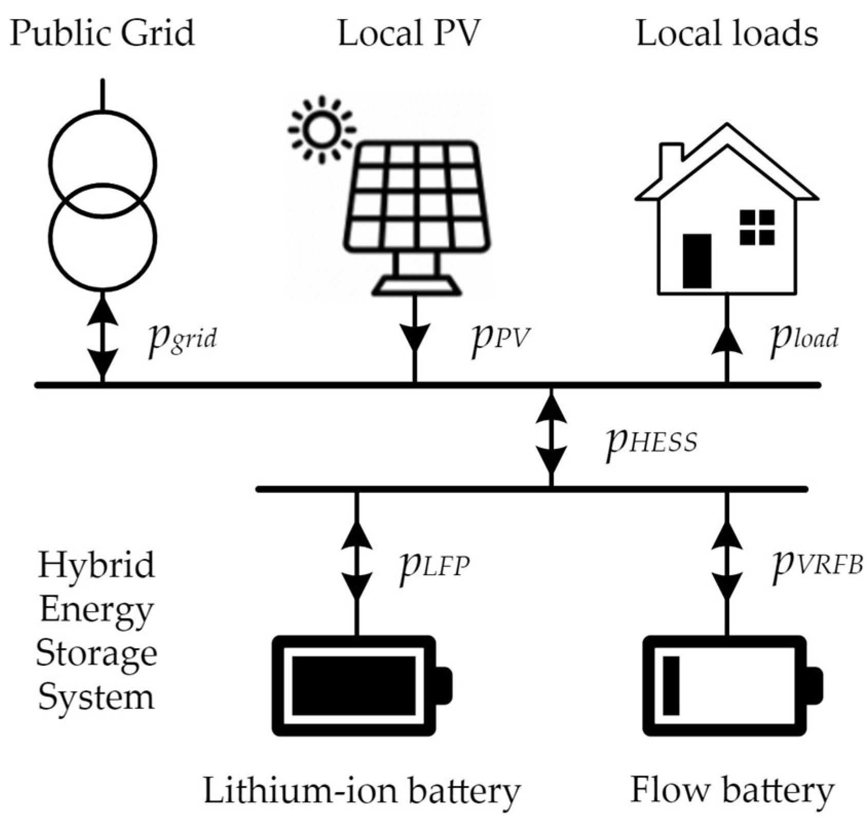
2.1. HESS Model

The setup considered in this work was a scenario of a microgrid that is equipped with RES; in the presented case, this was in the form of a photovoltaic (PV) installation. The system was equipped with a behind-the-meter HESS as shown in Figure 1.

Energy profiles were extracted from the historical data recorded by power analyzers at the KEZO Research Centre, Jabłonna, Poland. The usage was gathered from 3 buildings, which had laboratories, conference rooms, kitchens, bathrooms, administration offices, hotel rooms and a server room. The annual consumption was around 221 MWh; it was characterized with irregular patterns of usage—there were long intervals with a very high level of usage, but also non regularly appearing peaks. The usage was variable, ranging from 10 kW to 60 kW, with two dominating values around 20 kW and 38 kW (Figure 2). The centre was equipped with PV installations amassing 180 kWp in total, generating 144 MWh annually. The profiles of power generation and usage were aggregated in 15 min intervals, which is a commonly used interval of energy data gathering and it is consistent with the standard output of the energy meters. The usage and production aggregated per month is presented in Figure 3.

The HESS installed and used in the KEZO power system and modelled in this work consisted of a vanadium redox flow battery (VRFB) and a lithium-iron-phosphate (LFP) battery. The parameters of HESS batteries used for simulations are given in

Table 1. Hybrid energy storage system parameters assumed for the simulation.

Parameter	Symbol	Unit	VRFB	LFP
Installed capacity	Ebol	kWh	100	54
Max. continuous power	Pmax	kW	15	32
Allowed depth of discharge	DoD	%	100	80
Nominal number of cycles	NoC	-	5200	2000
Round trip efficiency	RTE	%	68	86
Battery block replacement cost	ReC	PLN/system	166,000	60,750

. Generalized battery cost and performance (number of cycles, efficiency) data were based on [24]. The batteries were connected logically in one network and were managed by the EMS system installed on an industrial computer.

The model included linear battery degradation, which reflected the battery capacity loss during its usage and the cost of replacing the battery block ($Re{C}_i$) after exceeding nominal energy throughput (Th_i). To evaluate depreciation cost of operating the battery, the degradation cost was calculated by multiplying discharge energy by a degradation cost factor (DCF). This factor was calculated as follows for each of the batteries (i—index of each battery in the HESS):

$$DC{F}_i=Re{C}_i/T{h}_i$$

(1)

where:

$$T{h}_i=No{C}_i\ast \left(Do{D}_i\ast E_{bol,i}\right)$$

(2)

The $T{h}_i$ is the nominal throughput of the storage calculated as the multiplication of number of cycles (NoC), depth of discharge (DoD) and the nominal capacity (E_bol)—the values for the considered setup are presented in Table 1.

The battery model also accounted for energy losses in the batteries. At the battery charging instants, a round trip efficiency (RTE) factor was applied to calculate the energy available for discharge.

For the sake of model simplification and reduction of computational burden, efficiency and degradation remained independent of the battery’s operational parameters, such as temperature, current and DoD.

The model was simulated with up-to-date Polish market prices in tariff B23, which is a real tariff for this type of building and usage. The energy tariff has three zones: the morning peak (from 7:00 until 12:00)—2.53 PLN/kWh, the evening peak (varies between seasons but ranges from 16:00 until 22:00)—3.43 PLN/kWh and the off-peak—1.96 PLN/kWh [25]. Surplus of energy was sold at the flat rate of 0.472 PLN/kWh [26]. The price profiles are depicted in Figure 4.

The aim was to show that the HESS can be economically justifiable and that it increases the self-consumption of the energy produced from the RES. The aim of the implemented optimization method was solely to minimize the cost of operation, a problem for which a solver was used. A simple control method—energy balancing—was given as a benchmark. Control methods are described in detail in the following sections. We assumed that the usage and production of the energy was not subject to changes. The only thing that changed the balance at the point of coupling with the grid was the operation of the HESS.

2.2. Energy Balancing

The benchmark method was chosen to represent the most simplistic operation of the ESS in the given setup. The idea of the basic energy balancing was very simple: the energy storage charges when production exceeds load and discharges when power was imported from the grid [27]. This control method minimized the exchange of energy with the external grid and did so without considering tariffs or even energy prices, thus foregoing possibilities for price arbitrage. On the other hand, such a method was guaranteed to use as much of the local RES overproduction as possible, in which case it potentially managed to increase self-consumption. In periods with low production from RES, the energy storage may not have a chance to charge. In our model, which assumed PV sources, this occurred in times with less sunshine, and, as a consequence, the HESS spent most of the winter time in a discharged state, thus not helping to decrease the costs of energy. On the upside, not using the battery implied that there is no degradation cost—the model is simplified and did not consider any degradation that might be caused by leaving the battery in an extremely low state of charge.

2.3. Economic Optimization

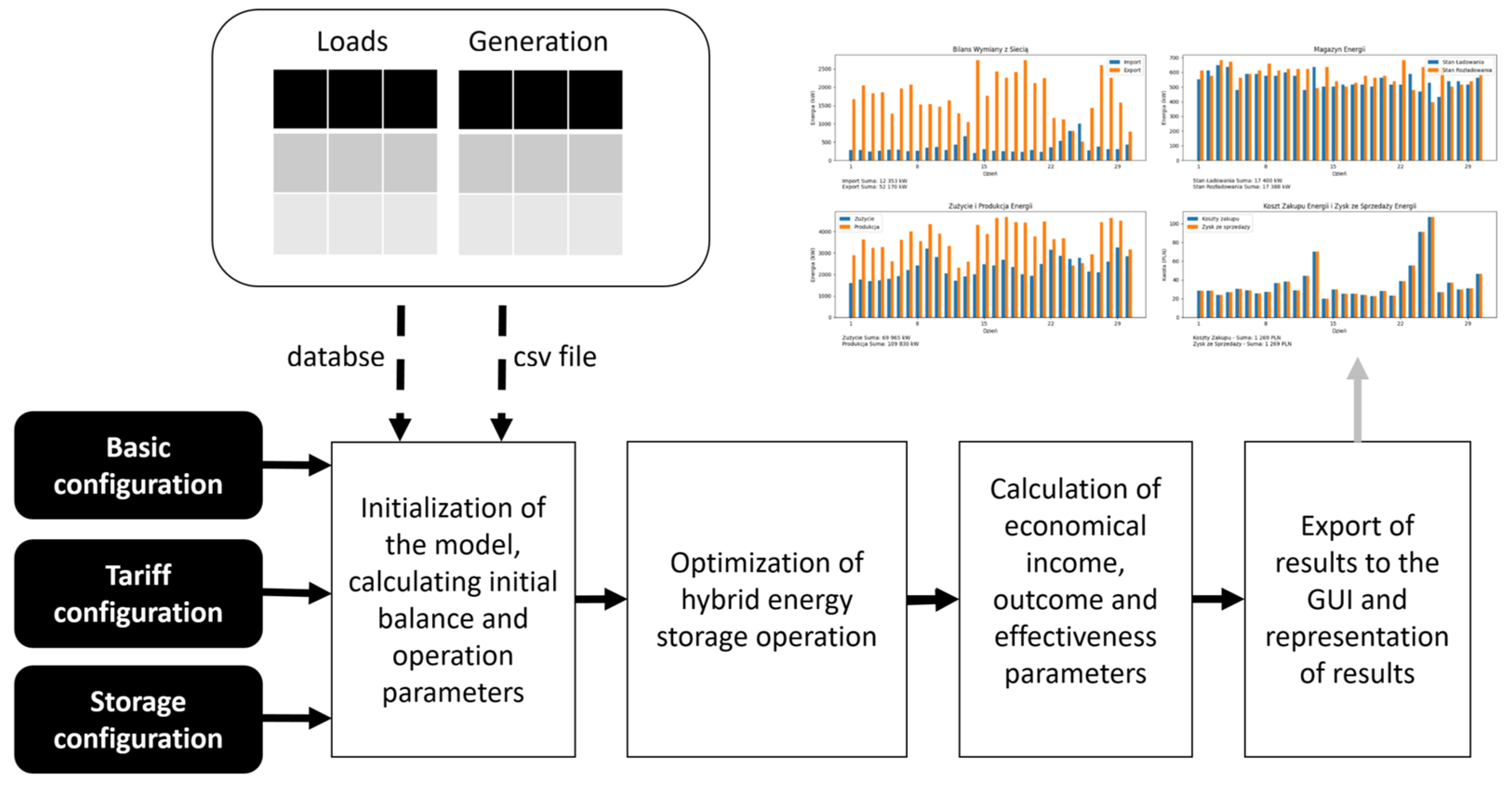
The operation of the HESS is described by its average power in a time period $t$ and denoted as $p_{HESS}\left(t\right)={\displaystyle \sum }_{i\in \left\{LFP, VRFB\right\}}{p}_i\left(t\right)$. The optimization happened in a time window, which had $T$ periods. Any length of time window can be chosen, but the size of this time window correlated with the duration of the computation: the longer the total time, the longer the computation will be. As we assumed that energy comes from PV and, in general, daily cycles are observed in usage patterns, it made sense to choose the total duration of $T$ as 24 h. To speed up the calculation of the solver, an initial solution was calculated and passed to the optimizer; this was a vector of length $T$ of values $p_i\left(t\right)$, where $i\in \left\{LFP, VRFB\right\}$. This initial solution suggested discharging at times of high-price tariff and charging in the low-price tariff. The gain in the time of calculation was small and neglectable. The grid balance at time $t$ was denoted by p_grid(t). The general rule was that the energy sent from the installation to the grid and the energy from the installation to the battery was positive; the energy taken from grid and the energy taken from the battery was negative.

The aim was to minimize the total balance that is influenced by the battery operation; therefore, the goal function $f_i$ was:

$$f_i={\displaystyle \sum }_{t=0}^T\{\begin{array}{c}\left|p_{grid}\left(t\right)+p_i\left(t\right)\right|\ast c_{buy}\left(t\right)+deg{r}_i\left(t\right), if \left(p_{grid}\left(t\right)+p_i\left(t\right)\right)>0\\ \left|p_{grid}\left(t\right)+p_i\left(t\right)\right|\ast c_{sell}\left(t\right)+deg{r}_i\left(t\right), if \left(p_{grid}\left(t\right)+p_i\left(t\right)\right)\le 0\end{array}$$

(3)

$$degr\left(t\right)=\{ \begin{array}{c}{p}_i\left(t\right)\ast DC{F}_i, if x_i\left(t\right)<0 \\ 0, if x_i\left(t\right)>0\end{array}$$

(4)

The goal function includes the tariffs: $c_{buy}\left(t\right)$ is the unit cost for buying energy from the grid for the given time frame t, and $c_{sell}\left(t\right)$ is the unit profit for selling energy to the grid. As we assumed that the tariff can change in each t, the main difference with peak shaving was that now it was not just the amount of energy that mattered at a time t, but this amount was linked via the tariff with the time at which it occurred. This combined energy with price, allowing an optimization for the general idea of reducing the amount of energy bought during price peaks with the aim of reducing the cost.

The constraints included the limitation for charging power:

$$\forall t:p_i\left(t\right)+p_{chg,i}>0$$

(5)

where $p_{chg,i}$ is the maximum power allowed for charging the battery.

Symmetrically there is a limitation for discharging power:

$$\forall t:p_{dchg,i}-p_i\left(t\right)>0$$

(6)

where $p_{dchg,i}$ is the maximum power allowed for discharging the battery. In the examples, $p_{chg,i}=p_{dchg,i}=P_{max,i}$.

Constraints of the state-of-charge (SOC) values were defined for each of the consecutive power values for energy storage at each time t. For not exceeding maximum state of charge, constraints were defined as follows:

$$\forall t:\left(E_{bol,i}-e_i\left(t\right)\right)-{\displaystyle \sum }_{j=0}^t{e}_i\left(j\right)>0$$

(7)

There are T-1 such constraints for charging the energy storage as power had to be recalculated to the equivalent energy $e\left(t\right)$ that was inserted into the battery. The charging energy was multiplied by the RTE value.

For not exceeding minimum state of charge, constraints were defined as follows:

$$\forall t:\left(e_i\left(t\right)-E_{bol,i}\ast \left(\frac{SO{C}_{min,i}}{100}\right)\right)+{\displaystyle \sum }_{j=0}^t{e}_i\left(j\right)>0$$

(8)

In this equation $e\left(t\right)$ is the energy that is discharged or charged, in case the charging of the RTE value is considered.

2.4. Implementation

The model was implemented in Python [28] as it is one of the popular languages with many well-implemented libraries. The libraries used were: pandas (which contains the very useful DataFrame structure that allows for database-like operation on data), numpy [29] (a package that contains a wide number of data structures and functions for data analysis and scientific methods), scipy [30] (which is equipped with a set of well-known optimization methods and also methods for interpolation and statistical analysis) and datetime (library for advanced operations on date–time formats).

The scheme of the software developed by the authors to run the technical and economic models, to calculate the optimization algorithm and to analyze and plot the results is illustrated in Figure 5. The model was designed to analyze the long-term (yearly) operation of the installation, and for that purpose a 15 min time-step was chosen, as it is a standard resolution of energy meters in Poland. This strictly binds the model to the data gathered in real systems.

The input data for the program were:

• The initial setup parameters, which included the general description of the microgrid parameters and date range for the simulation—the program allowed us to calculate the optimization for any data from a database or csv files.
• The information regarding energy prices—for the calculation of costs and revenues, it was necessary to have the full information regarding the zones, which can change monthly, and the prices of tariffs. The program has the ability to read the prices from a csv file in case there are dynamic tariffs; for the purpose of the project, the most typical Polish tariffs were implemented.
• The setup of the HESS—the parameters relevant for cost calculation and optimization of each battery that constitutes HESS had to be defined. The parameters were: the capacity, the maximum power of charging and of discharging, depth-of-discharge (DoD), number of cycles limit (NoC), round-trip efficiency (RTE), the capex cost and the cost ReC of replacing the battery unit when it reaches the end of its life.
• Time series of load and generation values for the installation—the required format consisted of separate files with a timestamp and average power in a row of csv files.
• The tariff profile file that consisted of a timestamp, the price for purchasing energy from the grid (or other entity in future, e.g., an aggregator) in PLN per kWh, the price for selling energy to the grid (or other) in PLN per kWh. It can represent dynamic tariffs [31] related to market or fixed peak hours tariffs. We assumed that changes can occur after a 15 min interval.

The data flow of the implemented model is schematically presented in Figure 5. The first stage is the initialization of a single DataFrame type structure with all the data indexed by a timestamp. Thanks to this, it is possible to make fast operations on columns and rows without the danger of missing the time alignment of the data. The program calculates initial balances of the energy p_grid that result from local load p_load and generation p_PV profiles and initializes structures for energy storage operation. The output data are the input to the optimization algorithm, which sequentially calculates the battery levels.

The program divides the data into 1-day-long chunks (starting from midnight) as daily patterns in usage are very often present and the production from PV modules has, by default, strong daily patterns.

Many different solvers were tested, the COBYLA [32] solver was the fastest in execution, but there were small fluctuations in the result that were not explainable in context of the test case. We chose SLSQP [33] as it is based on verified methods; for the considered problem, it should be effective in finding an optimal solution—if there is one—in reasonable time, without the need for extensive adjustments of the solver’s parameters. The SLSQP optimizer is a sequential least squares programming algorithm, it applies the Han–Powell quasi-Newton method with a Broyden–Fletcher–Goldfarb–Shanno algorithm update of the B-matrix and an L1-test function in the step-length algorithm. Its implementation contains a modified version of Lawson and Hanson’s nonlinear least-squares solver. The original source code was provided by Dieter Kraft in 1991, based on his work presented in [34]. The SLSQP was used in many publications in the domain of energy, e.g., [35,36]. The convergence and properties of the SLSQP are described in [37] and [38]. The parameters of the solver in this implementation were: maximum 500 iterations and the precision goal for the value of the goal function in the stopping criterion equals 0.1.

The optimization algorithm was called for each 24 h time window independently; only the final state of charge of each battery within HESS was passed to the next iteration. The outcome of the optimization was a time-series of the HESS operation—its discharge and charging power, change in the state of charge and amount of losses. Losses of the battery were defined as impacting the energy while charging—the program subtracts part of the energy that was equivalent to the 1–RTE.

The order of calculating the energy storage was defined by the durability of the battery, which was the nominal number of cycles NoC. The storage was ranked with this parameter, and the one with the highest value was considered first. This approach was chosen as a method to maximize overall durability of the HESS. When the first energy storage was calculated, the program recalculated the balances to include the energy storage impact on the installation. Then, the optimizer started with the next battery in line. Due to the nature of applied batteries it was assumed that priority would go to VRFB because of its high cycle life, low power and large capacity. The LFP battery was calculated in the second step to supplement operation of energy storage when higher power was needed. After each round, the details on the operation of each battery were saved and were also aggregated to the operation of the whole hybrid storage, which consisted of the sum of charging power, discharging power and losses.

The last step was calculating the economic balance of the costs and revenues from the installation. This was calculated for two cases: (a) with HESS and (b) without HESS. On the side of the revenues was the energy that was sold to the grid, which was solely overproduction from the local energy sources. On the cost side was the energy that had to be bought from the grid, as well as the cost of the degradation of the batteries, which was calculated proportionally to the battery throughput.

The analysis of the complexity was performed. We used the O-notation, as defined in [39], as it is a known standard in the defining of algorithm’s complexity. In the balancing algorithm, the complexity depended only on the number of considered batteries (Nb) and number of days the calculation was performed for (n), the complexity is O(Nb×n) as the time of calculation of the operation plan for a battery was constant. The optimization method was different—it used a solver and the number of iterations varied depending on the shape of the goal function. The worst case scenario was when there was no convergence and solver reached the maximum number of iterations, which was set to 500. Given that the maximum number of iterations was limited, this can be treated as a constant factor, and according to the O-notation this means the complexity of the operation was also O(Nb×n).

To estimate the mean time of calculation, we checked the distribution of the number of iterations—the histogram is presented in Figure 6. The number of iterations in time for both batteries is presented in Figure 7. On average, the simulation takes 186 iterations for each 24h window, per battery.

3. Results

The annual energy balance without an energy storage system is presented in Figure 3. In the following sections, a series of the graphs to visualize the performance of the behavior of the HESS operating for a full year are presented. The performance of HESS governed by different algorithms is analyzed in daily and seasonal horizons. Annual results for each algorithm are summarized and discussed in Section 4.

To describe the context, the situation of energy flows and costs without any battery system is presented in Figure 8. It is clearly visible that in winter, the purchase of energy in different tariff zones is comparable to the duration of those zones in a day. In the summer months, the photovoltaic installation is producing enough energy to cover the morning peaks almost completely. However, the production cannot cover the evening peak tariffs. The overall cost balance for the year is PLN 295,000, which includes the purchase of energy and the selling of surpluses from PV production.

3.1. Energy Balancing

The first set presents the operation of the simple energy balancing algorithm. Figure 9 presents the performance indicators aggregated per month to give an overview of the whole year’s operation. It is clearly visible that in winter months (November to February) the role of the production from photovoltaic is marginal and almost all of the produced energy is used for the self-consumption. In winter, the energy storage has no chance to charge as there is no surplus of energy. From March to October the activity of the energy storage is substantial, yet still, the storage is not able to completely rule out any purchase energy from the grid for June and July. Figure 9d represents the monthly aggregation of the energy bought and sold; in summer both can occur: sale and purchase can be present in the same month as one month can contain days when there is enough power from RES to cover the usage and sell, but the month can also contain days that might be too cloudy, making it necessary to buy energy.

The more detailed view of each month gives a much better picture of the actual HESS performance. In Figure 10 and Figure 11, the two different months are presented—January is the month with minimal energy storage activity, and July is the month when a surplus of produced energy allows the storage to cover the energy use in the evenings. On the 1 January, due to the initial settings of the simulation, the batteries are charged up to 50%, which causes the discharge of the battery immediately. In the other days in January, PV generation does not exceed the load, so there is no ESS activity. In July, however, the situation is much more interesting—there are days where there is no need to buy energy from the grid (Figure 10d), which shows the real usefulness of the energy storage.

The following figures illustrate daily power profiles of the microgrid, including HESS. To fully illustrate behavior of control algorithms under different conditions, three days are chosen: 27 July with high PV generation (Figure 12), 4 October with medium PV generation (Figure 13) and 6 February with almost no PV generation (Figure 14). The dynamics of the different types of batteries are clearly visible—the VRFB has more capacity, which cannot be fully used due to its lower power. Very visible is the non-optimal behavior of immediately discharging the storage at the beginning of the day in case the batteries have not discharged during previous day. Night time is related to lowest energy prices, so such behavior is not economically justifiable.

In October, the situation is similar to the summer time—there is still enough PV production that allows using both batteries to reduce the power exchange with the grid—first the VRFB is discharging, later the LFP takes over.

In winter (Figure 14), the energy storage is not active as there is little overproduction to be used.

Figure 15 summarizes the financial aspect of the HESS operation. Figure 15a depicts cost of energy purchased in each tariff zone, which clearly demonstrates that the high afternoon peak is not avoided, especially in winter months. In summer months, the PV production combined with the storage can substantially reduce the exchange with the grid. The overall costs and profits are presented in Figure 15b showing that the overall financial outcome is positive in June. Figure 15c gives the values of the surplus RES energy used directly or captured by the HESS. It is calculated as the costs that would have been if there was no energy production. In Figure 15d, the costs saved by the energy storage are presented, this includes the costs that are caused by the degradation of the storage—it is calculated from the difference of the total outcome with and without HESS. The overall cost balance has substantially decreased compared to the situation without the batteries at all, the value is PLN 266,028. This clearly shows that even the simple algorithm of battery management can lower the yearly costs of the operation of the facility.

3.2. Economic Optimization

The method of economic optimization is focused on reducing the overall cost of operating of the facility; it should use the energy storage to decrease the usage during peak times and charge in case of surplus or during low-zones of the tariffs. Before the run of the experiments, an analysis of the tariff prices and the degradation costs showed that, according to the calculations, the VRFB should be profitable to use for arbitrage when low tariff and evening peak tariff is considered. It is not profitable to use this storage to move energy from the morning peak to evening peak. The LFP battery has a different degradation cost and RTE, which makes it useful to move energy from the low and morning peak tariff to the evening peak. The using of batteries to increase the surplus of energy produced by PV is always profitable. The execution of the program showed that, very rarely, there is problem with convergence, especially in days with high production from PV modules. On such days there is an excess of energy, which generally creates the multiple solutions that are equivalent for the optimizer.

A comparison of the balancing method and the economic optimization method showed that the latter uses HESS all year round (see Figure 16c). However, the energy purchase costs and sell profits are not much different compared to the balancing algorithm (Figure 16d).

The more detailed view of each month provides a much better picture of the actual performance. In January, the HESS uses a lot of the batteries but only to move energy from the expensive time of the day to the cheaper tariff times. There is almost no difference in the cash flow of selling energy, but there is a visible difference when the cost of buying energy from the grid is considered (Figure 17d).

In July, the situation is very different—the energy storage reduces bought energy and consumes less from the surplus of the produced energy (Figure 18a). The total sell profits are higher, but also the cost of import from the grid is higher (Figure 18d). The economic optimization method in certain situations is more costly compared to the energy balancing method; it is due to the limitation of the optimization process to 24 h; this is the reason for the modified economic optimization, which is described further in the next section.

Checking the details of the algorithms, a very clear difference can be seen in the example day in July (Figure 19)—the batteries are discharged slowly and their energy is almost uniformly distributed over the whole period where there is a need to decrease energy usage. Similarly, charging shows no extremes, the speed of charging is decreased but maintained for a longer time. Analyzing the behavior day by day, it is clear that the optimizer is considering the degradation costs—the batteries are charged only to the point that is necessary to cover the single day. On 27 July and 4 October, it is especially visible (Figure 20) that the state of charge of the batteries is not reaching the maximum levels, even when it is possible to fully charge from the surplus of produced energy. Generally, the optimizer finds solutions that require smaller power to charge or discharge batteries, which is positive from the durability of the batteries but does not use the full capacity of the batteries when it is possible to charge from the PVs.

During winter (Figure 21), the behavior of the batteries shows the typical schedule of the HESS operation used for price arbitrage. Batteries are being charged during off-peak hours, even if it means importing extra amounts of energy from the grid. During the morning peak, the HESS power remains close to zero, while in the evening peak the highest priced batteries are being discharged. Both the VRFB and the LFP battery follow similar patterns. This behavior is consistent with our assumptions, based on the difference in prices between the price zones in the tariff.

The economic factors clearly show that the economic algorithm that reduces the purchase of energy is the highest tariff (Figure 22a), at the same time increasing the use of energy from the lowest tariff, especially in winter months. The general costs of the system are smaller when compared to the situation without any energy storage and also lower than the benchmark. The arbitrage in winter is decreasing the overall cost of operation of the whole facility. The experiments revealed a problem in which the batteries do not charge fully in case of a surplus of energy (this situation is visible on Figure 19b). This is caused by the fact that there is no value for the optimizer to keep a higher state of charge of the batteries at the end of the day. To solve the issue, the obvious action would be to run the optimization for a longer period (e.g., a week, a month) but then the number of changing variables would be significantly increased, which would bring two problems: the problem with convergence and the extended time of computations.

3.3. Modified Economic Optimization

To deal with the problem of single-day optimization, a modification is proposed—the optimizer does not care about the state of charge of the battery at the end of the day, but for the next day it would be generally beneficial to have a higher state of charge, especially when there is a surplus of production that could have been used. To implement that, an extra rule was enforced after the optimization stage: when there is surplus of energy from the renewable sources, the battery will always try to use as much of this surplus as possible to charge. This modifies the solution returned by the solver in a way that the energy storage reaches the full state of charge faster and more often, which, in consequence, causes an increased state of charge of the energy storage at the end of the day. For the following day, the optimizer will be given this raised state of charge to start its calculations. We tested the solution and present the outcome on the following graphs—Figure 23, Figure 24, Figure 25, Figure 26, Figure 27, Figure 28 and Figure 29. Figure 23 presents the monthly aggregated data—the increase in the operation of the energy storage in the summer months is clearly visible in comparison with the optimization method without modification. What is more, the import of energy has decreased, and, as a consequence, the cost of imported energy is also lower.

The more detailed view of each month gives a much better picture of the actual performance. In January (Figure 24), there are no changes in comparison to the optimization method as there is no surplus of energy.

For the summer months, the differences are much more visible; the graph for July shows the reduction in import and export of energy from and to the grid (Figure 25a). The batteries are charging and discharging more (Figure 25c) and the cost of energy import has dropped (Figure 25d). In this case, the difference between the energy balancing method and the modified economic optimization is very small and is mainly caused by small oscillations of the solutions given by the optimizer when it failed to reach the optimum solution in the defined number of iterations.

In July, the increase in the amount and duration of the charging of both batteries is visible. More of the surplus from the PV production is used. By the end of the day, the state of charge of the VRFB is higher in comparison to economic optimization (Figure 26).

The operation on 4 October (Figure 27) and 6 February (Figure 28) is almost the same as in the economic optimization without modifications.

The economic indicators show very interesting changes—the modification is reducing the use of the energy from the evening peak tariff, decreasing the overall energy costs for the facility and increasing the savings from the PV production and the operation of the HESS. The differences are not very significant, but the improvement is very clear, albeit only in summer months.

4. Discussion

The overall aim of this work is to present an economic optimization algorithm for hybrid energy storage that will improve the financial outcome of the setup and show that the hybrid energy storage is a feasible solution to improve the self-consumption of energy from PV installation. The results of the simulations for the benchmark and the proposed HESS control strategies are summarized in

Table 2. Comparison of the control methods and the setup without storage.

	Unit	Without HESS	Energy Balancing	Economic Optimization	Modified Economic Optimization
Import of energy	[MWh]	138.4	115.86	123.59	122.38
Export of energy	[MWh]	−61.5	−30.68	−32.84	−31.08
Self-consumption rate	[%]	57.3	78.7	77.8	79.3
Energy balance	[MWh]	76.8	85.19	90.75	91.3
Cost of import	[PLN]	324,091	270,695	261,351	258,820
Profit from export	[PLN]	29,060	14,478	15,502	14,671
VRFB Charge energy	[MWh]		23.11	35.88	37.71
VRFB Discharge energy	[MWh]	−	15.78	24.45	25.71
VRFB Equivalent cycles	-	−	158	244	257
VRFB Expected Lifetime	[years]	−	33	21	20
VRFB Depreciation cost	[PLN]		5038	7804	8207
LFP Charge energy	[MWh]		7.78	17.78	18.21
LFP Discharge energy	[MWh]	−	6.79	15.33	15.78
LFP Equivalent cycles	-	−	126	284	292
LFP Expected Lifetime	[years]	−	16	7	7
LFP Depreciation cost	[PLN]		4773	10,778	11,096
Energy cost	[PLN]	295,031	256,217	245,850	244,150
Financial outcome (including battery depreciation)	[PLN]	295,031	266,028	264,432	263,453

.

The first part of the table focuses on the energy between the facility and the power grid. The batteries generally decrease the import and export of energy; the energy balancing approach is the most limited, due to the fact that it only operates on the surplus of the energy produced by the PV installation. The economic optimizations are realizing arbitrage all year round—buying energy when it is cheap and using it during peak times. The self-consumption rates are interesting—this is the percentage of the energy produced by the PV installation that was used within the installation, which show that, thanks to the batteries, over 77% of the produced energy is either directly consumed or stored for later use. The difference between the storage management methods in this context is very small, which shows that any storage increases the use of energy from PV and that the optimization algorithms are rationally using the surplus from the PV production.

The second section of Table 2 presents the costs of import and profit from the export of energy. Although profits from exports are clearly correlated with the self-consumption rate, the cost of imports are affected by the cost in tariff zones. Here, the energy balancing method has the highest cost but uses the lowest amounts of import, which clearly demonstrates that economic optimization methods manage to shift energy between the zones.

The subsequent section presents the summary of the batteries’ operation. Battery charge and discharge energy is accumulated over the year to estimate the annual throughput and calculate energy losses. Equivalent cycles are calculated using discharge energy, nominal capacity and DoD. This, in turn, is used to estimate the lifetime of each battery within HESS, allowing the estimation of the point in the investment horizon that replaces the battery blocks. The economic optimization approaches make much more use of the energy storage, and thus also shorten its lifetime.

The financial outcome accounts for energy trading costs (which include battery losses) and for the depreciation of each battery (to account for the cost of battery block replacement at the end of the expected battery lifetime). For comparison, the values of financial outcome without depreciation costs was presented as this better shows how much the depreciation of the battery costs.

Energy balancing uses every opportunity to charge batteries with surplus generation that would be exported otherwise. As soon as the load is larger than generation, stored energy is used to supply loads. Energy balancing does not cycle batteries at all in winter time, when the PV installation does not generate surplus energy. It can be assumed that a single battery performs on average one cycle every two days. As a result, the balancing algorithm generates almost no cost savings in the winter months when the HESS stays in an idle state.

By contrast, the economic optimization methods leads to heavy balancing of the batteries, resulting in the shortening of the expected lifetime. Additional cycles are caused by the fact that cost optimization implies time-of-use strategy that charges a battery in an off-peak tariff to use it during peaks. This results in increased energy losses and battery depreciation. The advantages of including time-of-use strategy are seen in the financial outcome. Figure 21 and Figure 29 confirm that the majority of energy consumed is drawn from the grid in the off-peak tariff. The HESS leads to cost savings all year round.

The optimization method has another significant advantage over the balancing algorithms that was not reflected in the costs: it results in the operation of the LFP battery with relatively lower power. This leads to operation of the battery at lower temperature, and thus to an increased lifespan. This phenomenon has not been captured by the model applied but is an important point to investigate in future works.

The modification of the optimization method was introduced to partly overcome the problems connected to optimizing in 24 h windows. This 24 h window limits the horizon of the optimizer to the end of the day, and as such the optimizer is unable to increase the state of charge of the HESS, even if this would be beneficial for the next day. The implemented modification improved the solution, but there might still be a slight improvement if the optimization was calculated using longer time windows.

In this work, we limited the calculations to a 24 h window because the optimizer was also intended to perform the on-line optimization for the continuous management of an energy storage using forecasts; reliable forecasts can, however, only be obtained for the next day. Additionally, we considered a single day time rational in the case of a setup with a PV installation. The calculations were performed on standard desktop computers (CPU i5 3.2 GHz, 16 GB RAM) and while the balancing algorithm calculation time was below a minute, the simulation of an entire year using the economic optimization methods took 24 h. There is no possibility to parallelize the computations for this simulation as the state of charge of the storage at the end of the day is an input for the next-day computation.

5. Conclusions

A valuable tool has been implemented to test, simulate and analyze the behavior of the modelled HESS with battery models. The tool integrates a techno-economical model of a microgrid, including loads and RES. The model includes two battery types with their respective round trip efficiencies and costs of depreciation related to battery degradation during cycling. This simulation tool facilitates the sizing of the HESS installation, as well as the development and testing of control algorithms for scheduling the HESS operation. The graphical interface allows easy provisioning of input data while also allowing a visualization and analysis of the output data. The authors have implemented HESS control methods, including a simple energy balancing algorithm and using an energy cost optimization. The model and methods have been tested with real energy profiles recorded at a research centre.

The results explain the difference between the tested methods. The simple balancing algorithm stores surplus RES energy in the HESS and increases self-consumption rate to reduce the cost of energy; it does not do arbitrage as such, as it does not care about prices or tariffs. The advantage of this algorithm is its simplicity and moderate financial outcomes–using energy storages with such an algorithm brings profits in comparison to the setup without storage. The disadvantage is that this approach relies on the surplus of RES energy, otherwise the batteries are not used at all. Such an algorithm can be profitable when the averaged production from RES exceeds the usage of the facility. The economical optimization method on the other hand minimizes the costs of the operation during a single day. It uses the fact that there is a sufficient difference in cost of energy in different zones of the tariffs–using batteries for arbitrage can become profitable.

The total cost of using the VRFB battery (taking into account depreciation cost and losses related to the round trip efficiency) is not compensated by the difference between the prices in morning peak and off peak tariff zones. Adding an LFP battery, which has different properties and therefor cost balance, allows for reducing usage in all price peaks. The combination of both batteries allow to improve the cost balance of the operation and prolong the lifetime of the batteries.

In the presence of overproduction of PV installation, the simple balancing algorithm at times outperformed the economical optimization method. The reason for this is that the methods employ a 24 h time window, during which the simple balancing algorithm tried to charge the battery as much as possible (it did not count the cost), whereas the economical optimization limited the charging to what was necessary for this day. This meant that in the economical optimization, a subsequent day might start with a lower SOC level, even though there was the potential to charge them the day before. To compensate for this, a modification of the economic optimization was performed, where the surplus of energy in a day was used to charge the HESS as much as possible. This modification improved the economical optimization method compared to the simple balancing algorithm.

The economical optimization method uses the HESS for arbitrage and, as a result, causes a more intense cycling of both batteries within the HESS. The simulation with realistic technical and economic data show that the arbitrage introduced by the economic optimization method has a small effect on the overall financial result. Although the energy consumption in the peak hours, and thus the energy cost, is reduced, there are additional costs of battery depreciation and energy losses in the batteries. The potential for energy price reduction comes at a cost—the final economic result is only slightly better than the simple energy balancing when the battery depreciation cost is included. It should be noted that the impact of leaving a battery in a discharged state, which happens during winter months in the simple energy balancing, is not considered in the model.

Obviously, the financial results depend on a variety of factors, such as battery performance and cost, energy usage and generation patterns and most of all energy price profiles. For this reason, future work includes analyzing different HESS operating scenarios and adjusting the optimization method to take into account additional services that the HESS can provide.

The designed methods will be tested in a real environment with forecasted profiles being the basis for the optimizer. What is more, we plan to test the optimizer on the prices from the day-ahead market, where both the purchase and selling prices are changing every hour. The tool is intended to be further developed into a commercial tool for ESS installation planning and management. The tool will be modified to work with the predictions of load and production rather than with historic data, then it will become a scheduler that can be used to manage the operation of the energy storage, together with a real-time controller.

References

1. Armstrong, R.; Chiang, Y.-M.; Gruenspecht, H.; Brushett, F.; Deutch, J.; Engelkemier, S.; Gençer, E.; Jaffe, R.; Joskow, P.; Mallapragada, D.; et al. The Future of Energy Storage—An Interdisciplinary MIT Study. Report. 2022. Available online: https://energy.mit.edu/research/future-of-energy-storage/ (accessed on 30 August 2022).
2. European Association of Storage for Energy. Energy Storage Targets 2030 and 2050 Ensuring Europe’s Energy Security in a Renewable Energy System. 2022. Available online: https://ease-storage.eu/publication/energy-storage-targets-2030-and-2050/ (accessed on 30 August 2022).
3. IEA. Grid-Scale Storage; IEA: Paris, France, 2022; Available online: https://www.iea.org/reports/grid-scale-storage (accessed on 30 August 2022).
4. Hannan, M.A.; Wali, S.B.; Ker, P.J.; Rahman, M.S.A.; Mansor, M.; Ramachandaramurthy, V.K.; Muttaqi, K.M.; Mahlia, T.M.I.; Dong, Z.Y. Battery energy-storage system: A review of technologies, optimization objectives, constraints, approaches, and outstanding issues. J. Energy Storage 2021, 42, 103023. [Google Scholar] [CrossRef]
5. Miao, Y.; Chen, T.; Bu, S.; Liang, H.; Han, Z. Co-Optimizing Battery Storage for Energy Arbitrage and Frequency Regulation in Real-Time Markets Using Deep Reinforcement Learning. Energies 2021, 14, 8365. [Google Scholar] [CrossRef]
6. Yang, Y.; Lian, C.; Ma, C.; Zhang, Y. Research on Energy Storage Optimization for Large-Scale PV Power Stations under Given Long-Distance Delivery Mode. Energies 2020, 13, 27. [Google Scholar] [CrossRef] [Green Version]
7. Chen, Y.-T.; Kuo, C.-C.; Jhan, J.-Z. Research on Energy Storage Optimization Operation Schedule in an Island System. Appl. Sci. 2021, 11, 3690. [Google Scholar] [CrossRef]
8. Luo, L.; Abdulkareem, S.S.; Rezvani, A.; Miveh, M.R.; Samad, S.; Aljojo, N.; Pazhoohesh, M. Optimal scheduling of a renewable based microgrid considering photovoltaic system and battery energy storage under uncertainty. J. Energy Storage 2020, 28, 101306. [Google Scholar] [CrossRef]
9. Wang, Y.; Tian, J.; Sun, Z.; Wang, L.; Xu, R.; Li, M.; Chen, Z. A comprehensive review of battery modeling and state estimation approaches for advanced battery management systems. Renew. Sustain. Energy Rev. 2020, 131, 110015. [Google Scholar] [CrossRef]
10. Wang, L.; Li, M.; Chen, Z. An Energy Management Strategy for Hybrid Energy Storage Systems coordinate with state of thermal and power. Control Eng. Pract. 2022, 122, 105122. [Google Scholar] [CrossRef]
11. Lai, C.S.; Locatelli, G.; Pimm, A.; Wu, X.; Lai, L.L. A review on long-term electrical power system modeling with energy storage. J. Clean. Prod. 2021, 280, 124298. [Google Scholar] [CrossRef]
12. Katiraei, F.; Iravani, R.; Hatziargyriou, N.; Dimeas, A. Microgrids management. IEEE Power Energy Mag. 2008, 6, 54–65. [Google Scholar] [CrossRef]
13. Zia, M.F.; Elbouchikhi, E.; Benbouzid, M. Microgrids energy management systems: A critical review on methods, solutions, and prospects. Appl. Energy 2018, 222, 1033–1055. [Google Scholar] [CrossRef]
14. Meng, L.; Sanseverino, E.R.; Luna, A.; Dragicevic, T.; Vasquez, J.C.; Guerrero, J.M. Microgrid supervisory controllers and energy management systems: A literature review. Renew. Sustain. Energy Rev. 2016, 60, 1263–1273. [Google Scholar] [CrossRef]
15. Menniti, D.; Pinnarelli, A.; Sorrentino, N.; Vizza, P.; Burgio, A.; Brusco, G.; Motta, M. A Real-Life Application of an Efficient Energy Management Method for a Local Energy System in Presence of Energy Storage Systems. In Proceedings of the IEEE International Conference on Environment and Electrical Engineering and 2018 IEEE Industrial and Commercial Power Systems Europe (EEEIC/I&CPS Europe), Palermo, Italy, 12–15 June 2018. [Google Scholar] [CrossRef]
16. Wang, Y.; Liu, K.; Tang, X.; Dong, G. Editorial: Hybrid energy storage systems: Materials, devices, modeling, and applications. Front. Energy Res. 2022, 10, 1–3. [Google Scholar] [CrossRef]
17. Hajiaghasi, S.; Salemnia, A.; Hamzeh, M. Hybrid energy storage system for microgrids applications: A review. J. Energy Storage 2019, 21, 543–570. [Google Scholar] [CrossRef]
18. Tahir, Y.; Nadeem, M.F.; Ahmed, A.; Khan, I.A.; Qamar, F. A Review on Hybrid Energy Storage Systems in Microgrids. In Proceedings of the 3rd International Conference on Computing, Mathematics and Engineering Technologies (iCoMET), Sukkur, Pakistan, 29–30 January 2020. [Google Scholar] [CrossRef]
19. Tabart, Q.; Vechiu, I.; Etxeberria, A.; Bacha, S. Hybrid Energy Storage System Microgrids Integration for Power Quality Improvement Using Four-Leg Three-Level NPC Inverter and Second-Order Sliding Mode Control. IEEE Trans. Ind. Electron. 2018, 65, 424–435. [Google Scholar] [CrossRef]
20. Li, F.; Xie, K.; Yang, J. Optimization and Analysis of a Hybrid Energy Storage System in a Small-Scale Standalone Microgrid for Remote Area Power Supply (RAPS). Energies 2015, 8, 4802–4826. [Google Scholar] [CrossRef]
21. Bharatee, A.; Ray, P.K.; Subudhi, B.; Ghosh, A. Power Management Strategies in a Hybrid Energy Storage System Integrated AC/DC Microgrid: A Review. Energies 2022, 15, 7176. [Google Scholar] [CrossRef]
22. Gan, L.K.; Reniers, J.; Howey, D. A hybrid vanadium redox/lithium-ion energy storage system for off-grid renewable power. In Proceedings of the IEEE Energy Conversion Congress and Exposition (ECCE), Cincinnati, OH, USA, 1–5 October 2017. [Google Scholar] [CrossRef]
23. Qiu, X.; Nguyen, T.A.; Crow, M.L. Heterogeneous Energy Storage Optimization for Microgrids. IEEE Trans. Smart Grid 2016, 7, 1453–1461. [Google Scholar] [CrossRef]
24. Viswanathan, V.; Mongird, K.; Franks, R.; Li, X.; Sprenkle, V.T. 2022 Grid Energy Storage Technology Cost and Performance Assessment. Available online: https://www.pnnl.gov/sites/default/files/media/file/ESGC%20Cost%20Performance%20Report%202022%20PNNL-33283.pdf (accessed on 30 August 2022).
25. Energa Obrót. Standard Energy Prices for Commercial Customers Valid from 17.08.2022. Available online: https://www.energa.pl/dam/jcr:ae1072bf-f32f-4a83-8a89-dda88aa03ffd/Cennik%20standardowy%20dla%20przedsi%C4%99biorstw%20obowi%C4%85zuj%C4%85cy%20od%2017%20sierpnia%202022.pdf (accessed on 30 August 2022).
26. Urząd Regulacji Energetyki. Energy Market: The Average Energy Price on the Competitive Market in the Second Quarter of 2022 Was almost PLN 472/MWh. Available online: https://www.ure.gov.pl/pl/urzad/informacje-ogolne/aktualnosci/10551,Rynek-energii-srednia-cena-energii-na-rynku-konkurencyjnym-w-drugim-kwartale-202.html (accessed on 30 September 2022).
27. Yang, Y.; Li, H.; Aichhorn, A.; Zheng, J.; Greenleaf, M. Sizing Strategy of Distributed Battery Storage System With High Penetration of Photovoltaic for Voltage Regulation and Peak Load Shaving. IEEE Trans. Smart Grid 2014, 5, 982–991. [Google Scholar] [CrossRef]
28. Available online: https://www.python.org/ (accessed on 30 August 2022).
29. Available online: https://numpy.org/ (accessed on 30 August 2022).
30. Available online: https://scipy.org/ (accessed on 30 August 2022).
31. Eid, C.; Koliou, E.; Valles, M.; Reneses, J.; Hakvoort, R. Time-based pricing and electricity demand response: Existing barriers and next steps. Util. Policy 2016, 40, 15–25. [Google Scholar] [CrossRef] [Green Version]
32. Powell, M.J. A Direct Search Optimization Method That Models the Objective and Constraint Functions by Linear Interpolation. In Advances in Optimization and Numerical Analysis: Mathematics and Its Applications; Springer: Dordrecht, The Netherlands, 1994; pp. 51–67. [Google Scholar] [CrossRef]
33. SLSQP Documentation of Python Scipy Package. Available online: https://docs.scipy.org/doc/scipy/reference/optimize.minimize-slsqp.html#optimize-minimize-slsqp (accessed on 30 August 2022).
34. Dieter Kraft: A Software Package for Sequential Quadratic Programming; DFVLR-FB 88-28; DLR German Aerospace Center: Cologne, Germany, 1988.
35. Fracas, P.; Camarda, K.V.; Zondervan, E. Shaping the future energy markets with hybrid multimicrogrids by sequential least squares programming. Phys. Sci. Rev. 2021, 6, 20200050. [Google Scholar] [CrossRef]
36. Fracas, P.; Zondervan, E.; Franke, M.; Camarda, K.; Valtchev, S.; Valtchev, S. Techno-Economic Optimization Study of Interconnected Heat and Power Multi-Microgrids with a Novel Nature-Inspired Evolutionary Method. Electronics 2022, 11, 3147. [Google Scholar] [CrossRef]
37. Carrier, G.; Destarac, D.; Dumont, A.; Méheut, M.; El Din, I.S.; Jacques, P.; Saloua, K.; Brezillon, J.; Pestana, M. Gradient-Based Aerodynamic Optimization with the elsA Software. In Proceedings of the 52nd AIAA Aerospace Sciences Meeting—AIAA Science and Technology Forum and Exposition, SciTech 2014, National Harbor, MD, USA, 13–17 January 2014. [Google Scholar] [CrossRef] [Green Version]
38. Zahery, M.; Maes, H.; Neale, M. CSOLNP: Numerical Optimization Engine for Solving Non-linearly Constrained Problems. Twin Res. Hum. Genet. 2017, 20, 290–297. [Google Scholar] [CrossRef] [PubMed]
39. Cormen, T.H.; Leiserson, C.E.; Rivest, R.L.; Stein, C. Introduction to Algorithms; The MIT Press: Cambridge, MA, USA, 2001; ISBN 0262032937. [Google Scholar]
Figure 1. The schematic model of the HESS operating in a microgrid.
Applsci 13 00518 g001
Figure 2. The histogram of power of consumption in the used example in KEZO Research Centre.
Applsci 13 00518 g002
Figure 3. The energy of usage and production aggregated by month (data from the KEZO Research Centre).
Applsci 13 00518 g003
Figure 4. The price tariff for the selling and purchase of energy to/from the grid for months October–March.
Applsci 13 00518 g004
Figure 5. The general scheme of the operation of the optimization method.
Applsci 13 00518 g005
Figure 6. The histogram of the number of iterations for the cost optimization method.
Applsci 13 00518 g006
Figure 7. The number of iterations for each day of calculation for the cost optimization method.
Applsci 13 00518 g007
Figure 8. Monthly economic indicators for the setup without HESS or any other energy storage: (a) purchase cost classified by tariff zones (tariff prices), (b) costs, profits and financial balance.
Applsci 13 00518 g008
Figure 9. Results for the energy balancing method, aggregated monthly: (a) grid energy balance, (b) energy usage and production (input data), (c) activity of the energy storage, (d) cost of purchased energy and profit for sold energy.
Applsci 13 00518 g009
Figure 10. Results for the energy balancing method—data for the month of January, aggregated per day: (a) grid energy balance, (b) energy usage and production (input data), (c) activity of the energy storage, (d) cost of purchased energy and profit for sold energy.
Applsci 13 00518 g010
Figure 11. Results for the energy balancing method—data for the month of July, aggregated per day: (a) grid energy balance, (b) energy usage and production (input data), (c) activity of the energy storage, (d) cost of purchased energy and profit for sold energy.
Applsci 13 00518 g011
Figure 12. Results for the energy balancing method—data for 27 July: (a) grid power balance, (b) energy usage and production (input data), (c) batteries power, (d) batteries state of charge.
Applsci 13 00518 g012
Figure 13. Results for the energy balancing method—data for 4 October: (a) grid power balance, (b) energy usage and production (input data), (c) batteries power, (d) batteries state of charge.
Applsci 13 00518 g013
Figure 14. Results for the energy balancing method—data for 6 February: (a) grid power balance, (b) energy usage and production (input data), (c) batteries power, (d) batteries state of charge.
Applsci 13 00518 g014aApplsci 13 00518 g014b
Figure 15. Results for the energy balancing method—monthly economic indicators: (a) purchase cost classified by tariff zones (tariff prices), (b) costs, profits and financial balance, (c) costs of energy saved by PV generation, (d) costs of energy saved by HESS operation.
Applsci 13 00518 g015
Figure 16. Results for the economic optimization method, aggregated monthly: (a) grid energy balance, (b) energy usage and production (input data), (c) activity of the energy storage, (d) cost of purchased energy and profit for sold energy.
Applsci 13 00518 g016
Figure 17. Results for the economic optimization method—data for the month of January, aggregated per day: (a) grid energy balance, (b) energy usage and production (input data), (c) activity of the energy storage, (d) cost of purchased energy and profit for sold energy.
Applsci 13 00518 g017aApplsci 13 00518 g017b
Figure 18. Results for the economic optimization method—data for the month of July, aggregated per day: (a) grid energy balance, (b) energy usage and production (input data), (c) activity of the energy storage, (d) cost of purchased energy and profit for sold energy.
Applsci 13 00518 g018
Figure 19. Results for the economic optimization method—data for 27 July: (a) grid power balance, (b) energy usage and production (input data), (c) batteries power, (d) batteries state of charge.
Applsci 13 00518 g019
Figure 20. Results for the economic optimization method—data for 4 October: (a) grid power balance, (b) energy usage and production (input data), (c) batteries power, (d) batteries state of charge.
Applsci 13 00518 g020
Figure 21. Results for the economic optimization method—data for 6 February: (a) grid power balance, (b) energy usage and production (input data), (c) batteries power, (d) batteries state of charge.
Applsci 13 00518 g021
Figure 22. Results for the economic optimization method—monthly economic indicators: (a) purchase cost classified by tariff zones (tariff prices), (b) costs, profits and financial balance, (c) costs of energy saved by PV generation, (d) costs of energy saved by HESS operation.
Applsci 13 00518 g022
Figure 23. Results for the economic optimization method with modifications, aggregated monthly: (a) grid energy balance, (b) energy usage and production (input data), (c) activity of the energy storage, (d) cost of purchased energy and profit for sold energy.
Applsci 13 00518 g023
Figure 24. Results for the economic optimization method with modifications—data for the month of January, aggregated per day: (a) grid energy balance, (b) energy usage and production (input data), (c) activity of the energy storage, (d) cost of purchased energy and profit for sold energy.
Applsci 13 00518 g024aApplsci 13 00518 g024b
Figure 25. Results for the economic optimization method with modifications—data for the month of July, aggregated per day: (a) grid energy balance, (b) energy usage and production (input data), (c) activity of the energy storage, (d) cost of purchased energy and profit for sold energy.
Applsci 13 00518 g025
Figure 26. Results for the economic optimization method with modifications—data for 27 July: (a) grid power balance, (b) energy usage and production (input data), (c) batteries power, (d) batteries state of charge.
Applsci 13 00518 g026aApplsci 13 00518 g026b
Figure 27. Results for the economic optimization method with modifications—data for 4 October: (a) grid power balance, (b) energy usage and production (input data), (c) batteries power, (d) batteries state of charge.
Applsci 13 00518 g027
Figure 28. Results for the economic optimization method with modifications—data for 6 February: (a) grid power balance, (b) energy usage and production (input data), (c) batteries power, (d) batteries state of charge.
Applsci 13 00518 g028
Figure 29. Results for the economic optimization method with modifications—monthly economic indicators: (a) purchase cost classified by tariff zones (tariff prices), (b) costs, profits and financial balance, (c) costs of energy saved by PV generation, (d) costs of energy saved by HESS operation.
Applsci 13 00518 g029