2.1. Multiphysics Simulation
The simulation analysis of electromagnetic induction heating involves the multiphysics coupling analysis of the electromagnetic heating [
18], in which the analysis of the electromagnetic field is based on Maxwell field equations summarized by Maxwell in the 19th century, including Gaussian law (1), Gaussian electromagnetic induction law (2), the Faraday law of electromagnetic induction (3), and the Ampere circuit law (4) [
19]. The differential form is as follows:
In the above equations, D represents the electric flux density, C/m2; B is magnetic flux density, T; E is electric field strength, V/m; H is magnetic field strength, A/m; J is conduction current, A; t is time, s; and ρ is the charge density, C/m3.
Of these,
D,
H, and
J can form the constitutive equation together with the dielectric constant
ε (F/m), magnetic permeability
μ (H/m)
, and electric conductivity
σ (S/m) of electromagnetic material properties as follows:
The heat transfer phenomenon occurring in induction heating is the heat conduction in the conductor, which can be expressed by the transient heat conduction Equation (8) used for all simulations as follows:
In this formula, T refers to temperature, K; ρ is density, kg/m³; Cp is the specific heat capacity, J/(kg·K); k is the thermal conductivity of the material, W/(m·K); and Q is Joule heat, J.
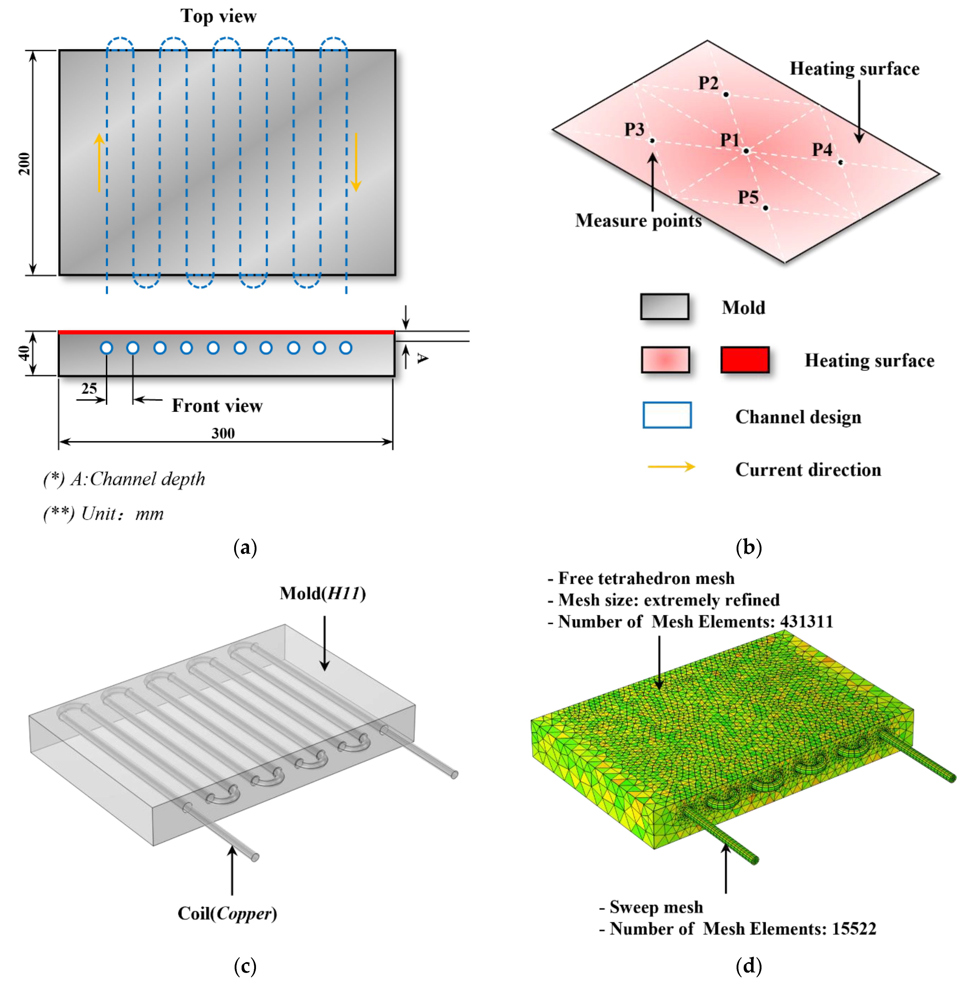
To obtain a simplified calculation model, CATIA software was used to draw the plate-type steel for the heating mold with a mold size of 300 mm × 200 mm × 40 mm. In addition, COMSOL Multiphysics software was introduced to simulate the mold surface temperature distribution and heating rate under three different conditions. A specific parameter range was set for a 30 KW induction heating power supply, with a maximum current of 1400 A when the equipment was running at full power, and a safety margin was set so that the current parameter was set to a maximum of 1200 A. As the induction coils needed to be fitted as close to the mold surface as possible, 5 mm to 9 mm was the ideal range to balance the heating effect with the mold structure. High frequency induction heating required an inductor frequency of 10 KHz or more, while a 30 KW induction heating power supply was set to a maximum regulation frequency of 50 KHz, so the frequency range was 20 KHz to 40 KHz. The parameters are set as follows: (1) The depths from the coil to the mold surface were set to be 5 mm, 7 mm, and 9 mm, respectively, to explore the influence of varying depths on the uniformity of the temperature distribution on the mold surface and the heating rate. The two-dimensional diagram of the mold is shown in
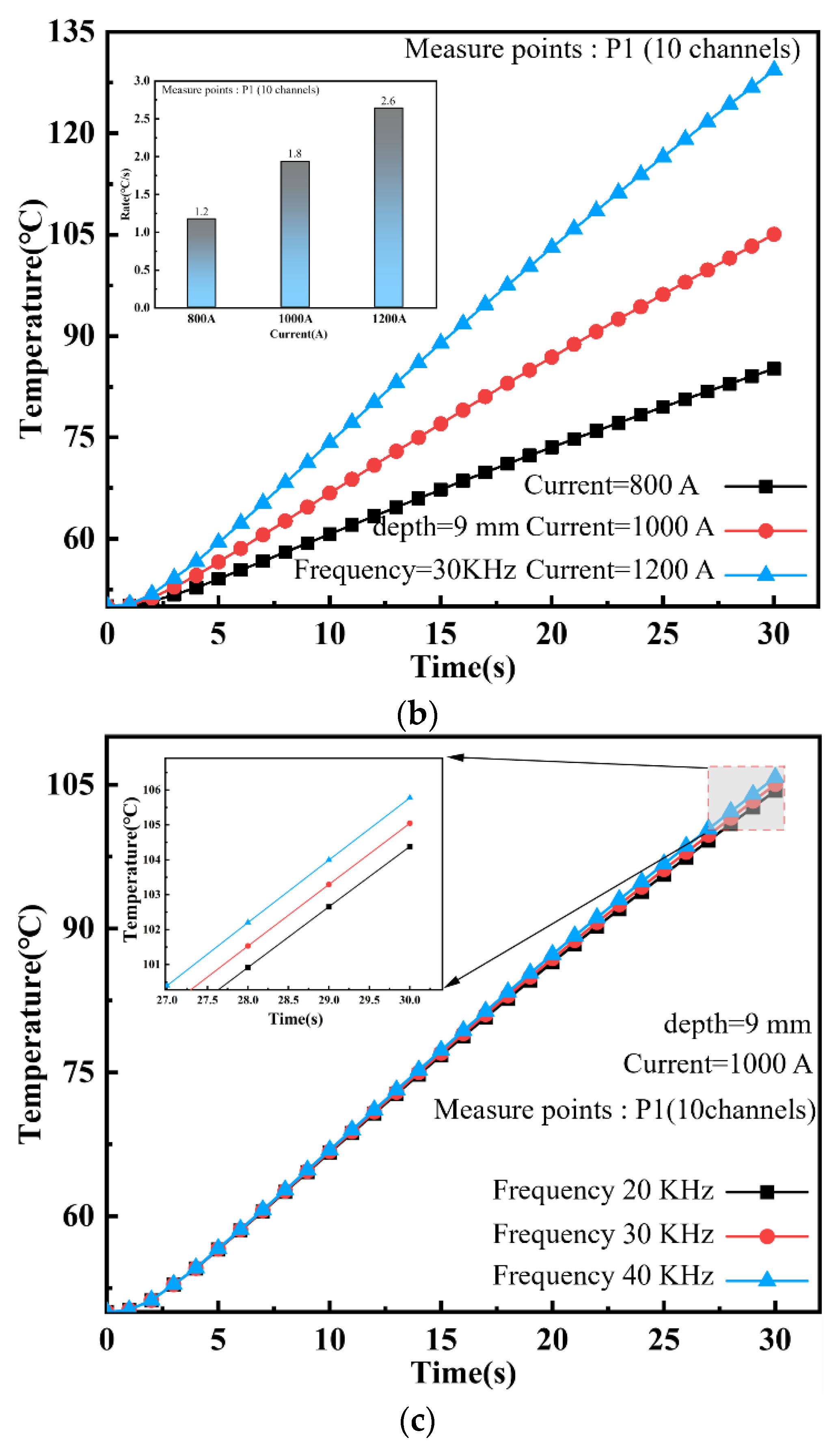
Figure 1a. As the inductors are made of soft coils and need to be mounted inside the mold, they need to be perforated inside the mold. This is the reason for using soft coils as inductors, which can be arranged at random inside the mold and reach the desired temperature of the mold. (2) The impact of different currents on the heating efficiency of the new induction heating coil was studied at following currents: 800 A, 1000 A, and 1200 A. (3) The frequencies were set to 20 KHz, 30 KHz, and 40 KHz, respectively, to discuss the effect of varying frequencies on this efficiency.
The temperature of 5 measuring points on the mold surface, as shown in
Figure 1b, was selected as the final result and the reference temperature of the mold surface. After heating for 30 s, the final temperature at these 5 points was obtained, and their mean temperature was calculated using Equation (9) and regarded as the final heating temperature of the mold.
Figure 1c shows a perspective view of the 3D simulation model with the induction coil interspersed in the interior of the mold, and
Figure 1d shows the mesh division. The focus of this simulation was to characterize the temperature distribution on the surface of the mold, therefore a very fine free tetrahedral mesh was used for the mold and, for the coil, a swept mesh with 15522 mesh elements was used, which reduces the pressure on the calculation run and speeds up the calculation time. The overall experimental scheme is shown in
Table 1.
In this equation, represents the mean temperature of 5 points; is the final heating temperature of each point; and n refers to the number of measuring points, which is set to be 5 in this experiment.
In this electromagnetic thermal multiphysics coupling, the low mold temperature has little influence on the mold material parameters even after it rises, the influence of which on the material parameters can be ignored as a result. The heat transfer mode of all external surfaces of the mold is set to free convection with air, the ambient temperature is 20 °C, and the heat transfer coefficient is 10 W/(m
2·K). The parameters of other air, mold, and induction coils are shown in
Table 2, where
μr is a relative dielectric constant;
σ represents the electric conductivity;
ρ refers to the density;
K is the electric conductivity; and
Cp is the heat capacity at constant pressure. The air and copper parameters are sourced from the COMSOL software’s own material library and H11 from Roctool’s actual mold parameters.
2.2. Taguchi Method and ANOVA
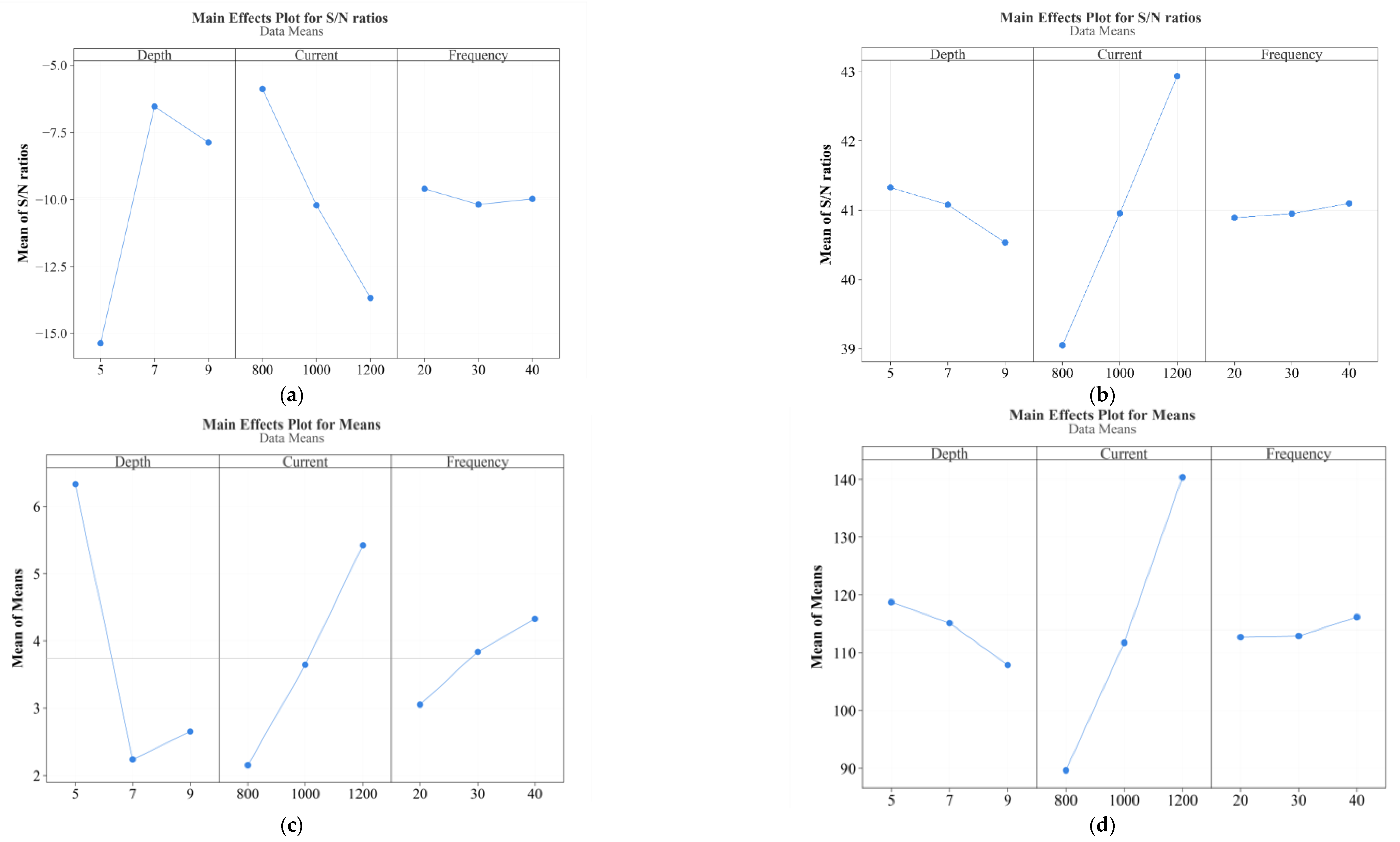
The Taguchi method, which was proposed by Dr. Genichi Taguchi of Japan, introduces the orthogonal table into experimental designs. It spread quickly around the world due to multiple advantages, including a high reproducibility of experimental results, a scalability of configuration experiments, a lower number of tests, simple operation, and easy configuration. Using this method, the optimal parameter combination under corresponding horizontal conditions can be realized through some experiments. In this study, the heating depth, current, and frequency were selected as parameters to carry out simulation experiments based on the L9 orthogonal table involving three factors and three levels that was designed by Taguchi method.
Table 3 presents the levels of three factors. The specific experimental design is shown in
Table 4. Finally, the experimental results were first analyzed based on the signal-to-noise (S/N) ratio and then divided by optimization objectives into three characteristics: nominal-the-best, larger-the-better, and smaller-the-better [
20], which correspond to Equation (10), Equation (11), and Equation (12), respectively:
In the above equations,
n represents the number of experiments in each group;
refers to the results of a single experiment; and
μ is the sample mean. It is necessary in this experiment that the higher the mean temperature after heating, the better, which is classified into the larger-the-better characteristic. The range of temperature at five points, denoted by
s, is calculated with Equation (13) and is used to characterize the temperature uniformity:
where
s represents the range of temperature at measuring points;
and
are maximum and minimum temperatures of these five points, respectively. Then, the extent to which each factor affects the experimental results is determined through the analysis of variance (ANOVA).


