Combining Standard Artificial Intelligence Models, Pre-Processing Techniques, and Post-Processing Methods to Improve the Accuracy of Monthly Runoff Predictions in Karst-Area Watersheds

Abstract

The complex and unique topography of karst regions highlights the weaknesses of traditional hydrological models which fail to fully generalize them. The successive proposals of standard artificial intelligence (AI) models, pre-processing techniques, and post-processing methods have provided new opportunities to enhance the accuracy of runoff prediction in karst areas. In this study, first, the BP neural network model and the Elman neural network model were used for runoff prediction. Then, the performance of four coupled models—formed by combining two AI pre-processing techniques, Empirical Modal Decomposition (EMD) and Ensemble Empirical Modal Decomposition (EEMD), with the previously mentioned AI models—was investigated. Finally, the accuracy of triple-coupled models, formed by applying the post-processing method of quantile mapping (QM) to the previous coupled models, was estimated. The Nash–Sutcliffe efficiency (NSE), the mean absolute percentage error (MAPE), the root mean square error (RMSE), and the peak percentage of threshold statistics (PPTS) were selected to evaluate and analyze the forecasting results of the above models. The results demonstrated that the BP model had the best prediction effect of the standard AI models, the coupled forecasting models had better prediction accuracy than the standard AI models, and the triple-coupled QM–EMD–Elman model had the best forecasting effect with an NSE value of 0.73, MAPE value of 0.75, RMSE value of 34.60, and PPTS value of 2.36.

1. Introduction

Water resources are vital to human survival and development, and are essential to sustainable development. Runoff changes affect issues such as reservoir operation and water resource allocation, which in turn affect society’s economic development [1]. With climate change and human activities becoming increasingly intense, runoff change has become an issue of great concern to hydrologists. Scholars in the field of hydrology have conducted a great deal of research that has promoted the rapid development of hydrological models. To summarize these previous scientific achievements, the existing popular hydrological models mainly include “process-driven models” and “data-driven models”. The “process-driven models” consist of experimental formulations based on physics [2], which are usually less scalable and less generalizable due to time and space constraints. By contrast, the main factor considered in “data-driven models” is not the natural hydrological cycle but the relationships that exist within hydrological data, which are then used to build optimal models of the data through iteration and adjustment of model parameters. “Standard artificial intelligence models” play a large part in the application of “data-driven models” and have great potential [3].

Standard artificial intelligence models have the advantages of ease of compatibility, operation, and implementation, so they are widely used in runoff prediction. Kieran et al. [4] used a long short-term memory neural network for runoff prediction in western U.S. rivers, showing the future promise of neural networks in hydrologic prediction. Sharifi et al. [5] explored the possibility of using the support vector machine (SVM) model in runoff prediction. From the results, it can be seen that the SVM model is not only suitable for small-sample situations, but also superior in terms of performance to other runoff-prediction techniques in the Amameh watershed. Based on normalized information measurement and dataset base transformation, Li et al. [6] proposed an adaptive runoff-prediction method using an Elman neural network (ENN), and evaluated the method using the runoff process of the Chengdu Hydropower Station from 2007 to 2011. The results showed that the maximum relative error of multiple predictions was less than 16% and that the prediction was excellent.

However, there is still much room for improvement, because traditional AI models have issues with parameter optimization and prediction accuracy; attempts to address these worries led to the creation of the coupled model. A large number of scholars have researched the combined predictions of standard AI models coupled with pre-processing techniques. Peng et al. [7] eliminated redundant noise from the original runoff sequence using the empirical wavelet transform (EWT), then identified the inputs of artificial neural network (ANN) models using a partial autocorrelation function, and finally used these to construct a hybrid EWT–ANN model. The hybrid model has been applied to runoff observations at four hydrological stations on the Yangtze River, China. Yuan et al. [8] investigated the accuracy of a hybrid model combining the long short-term memory model with the ant lion optimization model in monthly runoff predictions. The results demonstrated that this hybrid model had higher accuracy than the long short-term memory neural network model alone. In order to improve the accuracy of runoff prediction, some scholars apply post-processing methods to correct for deviation. Qu et al. [9] applied the Bayesian Model Averaging post-processing method to runoff predictions in the Ful River basin, and showed that this method could improve the performance of raw multi-model grand ensemble runoff predictions. Bogner et al. [10] conducted a study to improve the quality of low-flow predictions in several catchments in Switzerland. The results showed that the Quantile Regression Neural Networks method played a significant role in improving the prediction quality. The utilization of standard AI-based data-driven models for monthly runoff prediction can enhance the prediction effect, which is of great importance in the field of predicting hydrological runoff direction.

Karst areas account for 7–12% of the Earth’s continental area. About a quarter of the world population’s drinking water comes from karst aquifers [11]. Therefore, hydrological studies in karst areas are critical. Karst geology is widely distributed in China, and the distribution area of soluble rocks accounts for about 1/3 of the national land area. In the south of China, the distribution of karst areas is mainly in Yunnan and Guizhou provinces and Guangxi district. Additionally, the total area of karst in Guangxi is 120,000 km², accounting for half of the total area of Guangxi. Karst is formed by the dissolution of soluble rocks and its characteristics include sinkholes and caves in the underground drainage system [12]. The complex and unique topography of karst regions leads to difficulties for traditional hydrological models to fully generalize them, especially when the underlying physical relationships (or underground geographical characteristics) cannot be explicitly obtained. As can be seen in

Table 1. Application of hydrological models to karst areas.

Classification	Name	Author	Improvements	Advantages and Disadvantages
Lumped hydrological model	Xin’anjiang	Zhao et al. [18]	The conversion of surface flow to underground flow in karst areas of Central Guizhou Province was simulated.	Advantages: The Xin’anjiang model is simple in structure and fast in calculation. The Tank model overcomes to some extent the problems caused by turbulent flow in karst basins. Disadvantages: These models generally use empirical or lumped generalizations to describe runoff processes, the physical meaning of the parameters in the models is not clear, and the groundwater conditions in hydrological simulations using these models for karst basins may not match reality.
	Tank	Fleury et al. [19]	Used three interconnected tanks to represent the spatial layer structure of the karst water-bearing medium and simulated groundwater at different velocity. Application to Fontaine de Vaucluse (southern France).
Distributed hydrological model	SWAT	Palanisamy et al. [20]	The sinkhole diameter function was developed based on the flow through the sinkhole orifices in the streambed of the Kentucky karst basin. The function was added to the SWAT model to form a karst SWAT model.	Advantages: easy acquisition of data and high calculation efficiency. Ability to simulate different hydrological processes in large complex basins using spatial information provided by GIS and RS. Disadvantages: The SWAT model is difficult to use for short-term hydrological simulations; the model is based on the properties of loose media, which does not represent the characteristics of karst basins well; and there are limitations in the hydrological simulation of karst basins.
		Nikolaidis et al. [21]	Modified the input flows to the SWAT model for deep groundwater.
	TOPMODEL	Sun et al. [22]	Used the TOPMODEL model to carry out simulations of two topographic index models for homogeneous mountainous regions in the Suomo Basin.	Advantages: the model can be used for calculations in watersheds where no information is available, with a simple structure and fewer parameters. Disadvantages: due to complex topography in karst areas, karst water systems generated by the DEM model may not match reality.
	SWMM	Campbell et al. [23]	Used SWMM to simulate the flow process of water in karst in Stephens gap cave.	Advantages: It reflect a more realistic process of the flood waves through the pipeline. Disadvantages: SWMM is sensitive to the geometric features of the pipeline, and when applied to karst basins, it does not take into account the water exchange between the pipeline and the aquifer; and the physical mechanism needs to be improved.
	HEC-HMS	Dvory et al. [24]	Used the reservoir unit method to simulate the stagnation of water flow in karst basins.	Advantages: The model has good accuracy and is able to take into account subsurface changes in the study area, and is suitable for the simulation of runoff processes over short time periods. Disadvantages: Need to add the karst storage unit, and simulation results are unstable.

, traditional hydrological models are typically applied to specific watersheds and need large amounts of measurement information (or expert experience). Although runoff processes can be reflected in hydrologic models, measurement information and expert experience are often needed to dynamically adjust computational parameters and model structure [13]. Artificial intelligence models can provide new possibilities for runoff prediction when the underlying physical relationship cannot be explicitly obtained. However, few studies have investigated the effectiveness of artificial intelligence models for runoff prediction in karst areas. Meng et al. [14] applied artificial neural networks to a typical karst region in Hubei province, China; An et al. [15] constructed a model that combined Ensemble Empirical Mode Decomposition and the Long Short-Term Memory model to effectively improve the prediction accuracy of discharge from karst springs; Line et al. [16] used Lez basin in southern France as an example to verify the feasibility of applying neural network models to karst basins and proposed an effective method to determine the complexity of neural models; Mo et al. [17] measured the stability of models based on different data structure inputs and investigated the effect of input methods on the performance of AI models in karst areas. This study helps to further bridge this gap by first investigating the performance of standard AI models and pre-processing-technique-based AI methods in karst watershed modeling, before then demonstrating superiority of triple-coupled models that apply quantile mapping to these standard coupled methods.

In summary, although previous runoff prediction studies have achieved specific results, there are still many problems. Few studies have applied emerging artificial intelligence models to monthly runoff predictions in karst areas. In addition, no study has comprehensively evaluated the performance of coupled models formed by combining pre-processing techniques, artificial intelligence models, and quantile mapping post-processing methods to predict monthly runoff in karst areas. Therefore, this research mainly studies the effectiveness of traditional standard AI and pre-processing techniques in karst watershed modeling, as well as the superiority of applying quantile mapping post-processing to these coupled methods. For this purpose, the following research was carried out: first, monthly runoff predictions were conducted using the BP neural network model and the Elman neural network model; then, the performance of four coupled models (formed by combining two pre-processing techniques, Empirical Modal Decomposition (EMD) and Ensemble Empirical Modal Decomposition (EEMD), with the previously mentioned neural network models) were investigated; finally, the accuracy of triple-coupled models (formed by applying the post-processing method of quantile mapping (QM) to the coupled models) was estimated. The Nash–Sutcliffe efficiency (NSE), mean absolute percentage error (MAPE), and root mean square error (RMSE) were selected to evaluate and analyze the forecasting results of the above models, and the optimal model was determined.

2. Study Area and Data Source

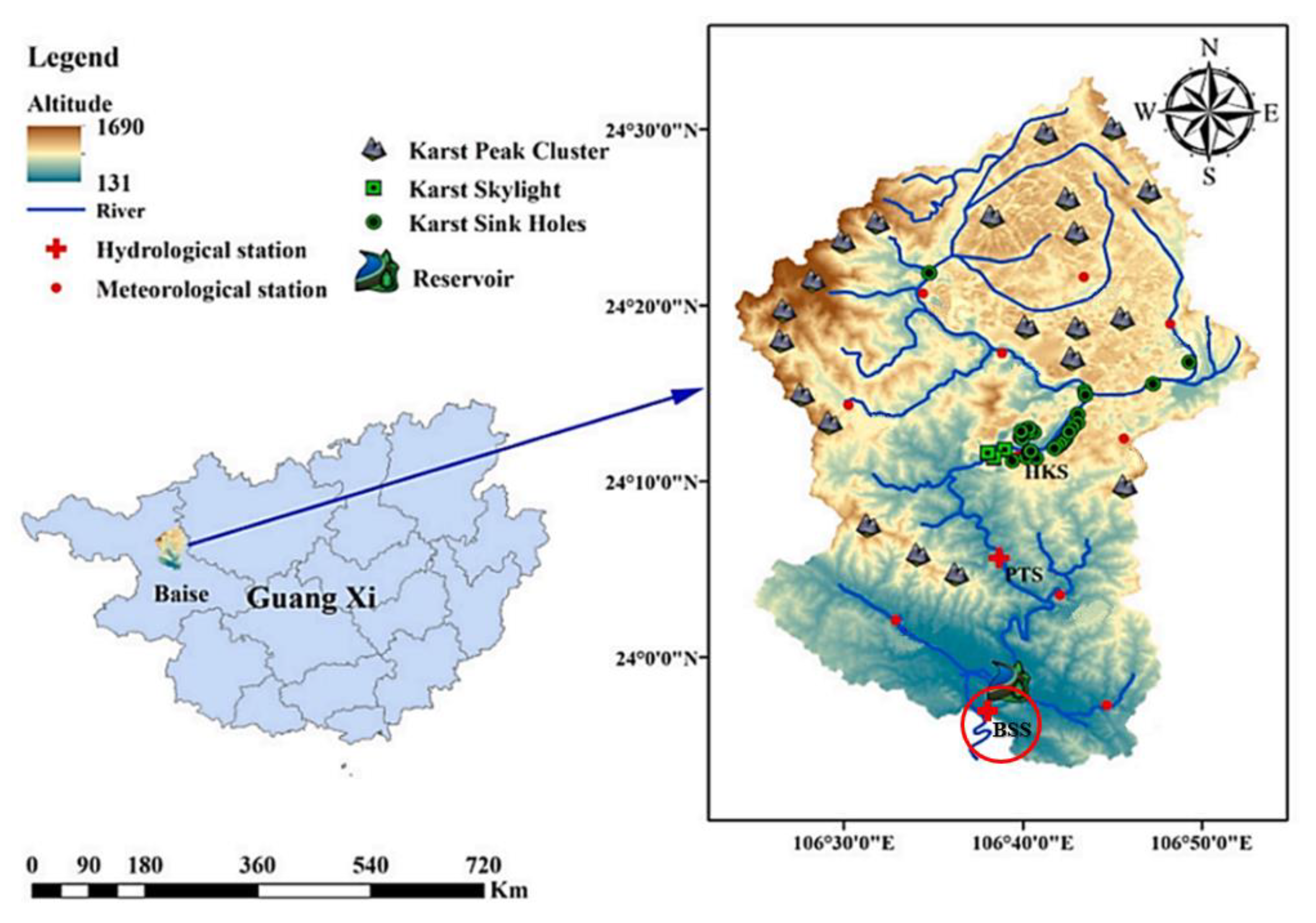
2.1. Study Area

The Chengbi River originates from the eastern foot of Qinglong Mountain within Lingyun County, located to the northeast of Baise city, Guangxi district, China. The geographical location of the Chengbi River watershed is shown in Figure 1. The drainage area of the Chengbi River basin is 2087 km², which is typical of a karst-area basin; karst geomorphic area occupies about 53.7% of the total area of the basin, while the total reservoir capacity is 1.15 billion m³, and the water surface area is 39.1 km². The unique features of this watershed are the numerous karst sinkholes, karst skylights, and karst peak clusters in the northern region, while the southern region mainly contains a karst peak clusters and a reservoir [25]. The Chengbi River basin is a typical karst basin, where the karst features on the surface are obvious, but the subsurface is not well understood, and the presence of the reservoir makes the runoff process more difficult to predict. This phenomenon is common in other karst watersheds [26]. Therefore, there is an urgent need to combine standard artificial intelligence models, pre-processing techniques, and post-processing methods to generate more accurate runoff predictions.

2.2. Data Source

There are three hydrological stations in the Chengbi River basin, namely Bashou, Pingtang, and Haokun. However, unlike the Bashou hydrological station, the other two stations were established relatively recently, so the recorded data from those stations covered a relatively short period of time. Therefore, the monthly runoff data from the Bashou station were used for analysis, providing a total of 492 months of data, from 1979 to 2019. The runoff data were provided by the Chengbi River Reservoir Authority by separating the run-off data of the designated section from the rainfall catchment area above the section. Before the runoff prediction, the amount of input data was determined in advance, and was used as the basis for prediction. Then, the following data were predicted and the optimal lag time was selected. When the amount of input data was small, the number of training times was low and the prediction effect was poor. When the amount of input data was too large, overfitting was easy and the prediction effect was also impacted. In this paper, by referring to the input lag time from the previous literature [27], 11 types of optimal sets (lag time of 1 to 11 months) were finally selected. After inputting the model for each scenario, the results under each scenario were obtained, and the final results were determined by comparing and selecting the preferences. After conducting several experiments, it was found that when the training set was divided from the validation set in a ratio of 8:2 [27], it was able to provide the training data needed to enable the machine learning algorithms to obtain lower error rates, as well as to achieve higher accuracy in the prediction of the validation dataset. In this case, the training set is divided from 1979/01 to 2011/10, and the validation set is divided from 2011/11 to 2019/12.

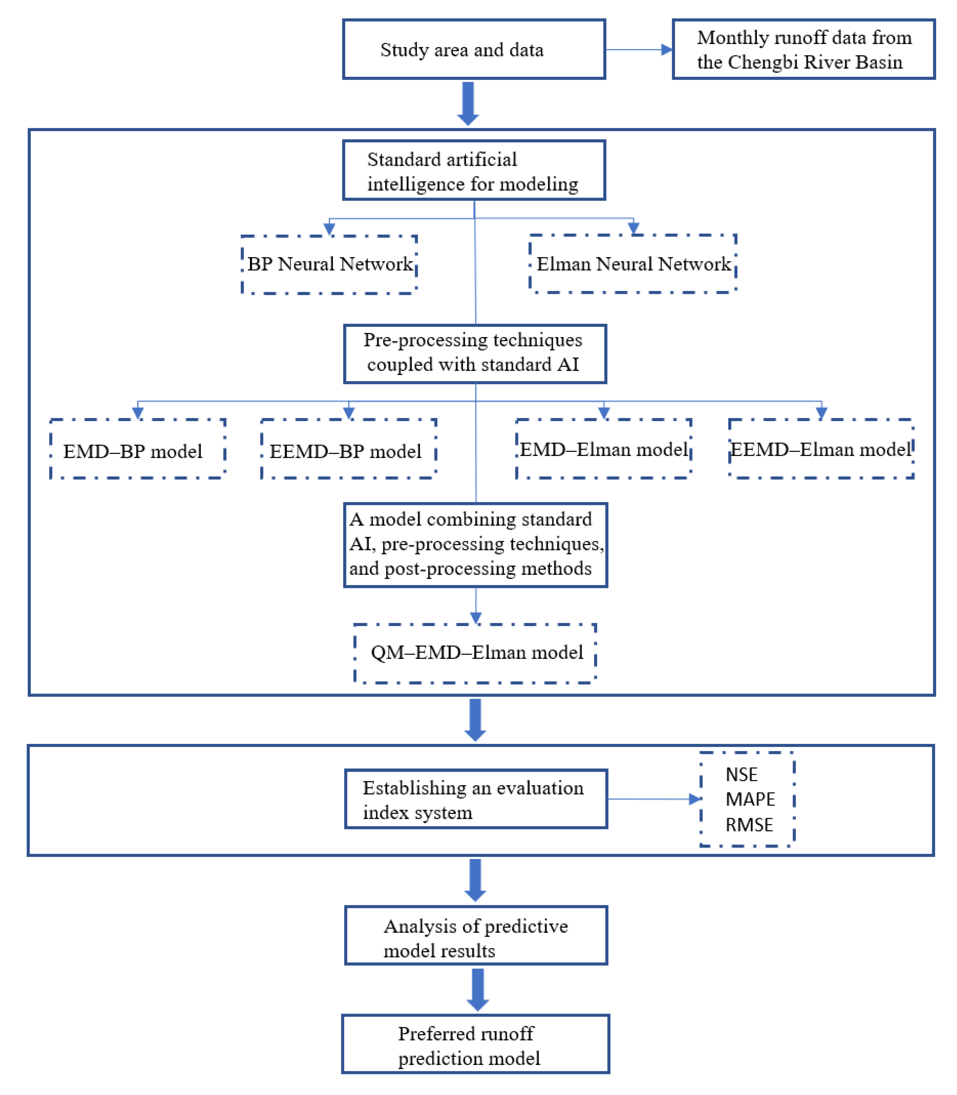
3. Methodology and Comparative Experimental Setup

The research idea and specific process of this paper are shown in Figure 2.

The methods used in this study consist mainly of the following two parts: (1) methodologies including pre-processing techniques, standard artificial intelligence models, and post-processing methods, and (2) comparative experimental setups including experimental setups and evaluation metrics. Due to space limitations, only the following methods are briefly described.

3.1. Methodology

3.1.1. Decomposition Method for Data Pre-Processing

• Empirical Mode Decomposition;

Empirical Mode Decomposition, which was proposed by Huang et al. [28], is an adaptive signal time-frequency analysis method that can extract the eigenmode function of the signal and its features. The EMD decomposition method can decompose the original signal into many components and name each component as an eigenmodal function, so it can be applied to the analysis of nonlinear and non-stationary signals [29]. The final decomposition result consists of the Intrinsic Mode Function (IMF) and the residual signal, and the decomposition result is expressed as follows [30]:

$$s\left(t\right)={\displaystyle \sum }_{i=1}^{n}im{f}_i\left(t\right)+r_n\left(t\right)$$

(1)

where $r_n\left(t\right)$ is the residual signal and $im{f}_i\left(t\right)$ is the IMF component of different frequency components from high to low.

Each IMF needs to satisfy the following conditions:

(1)

The number of zero-crossing points minus the number of extreme points ≤ 1 for all signals.

(2)

The average value of the upper and lower envelopes is 0 at every point.

• Ensemble Empirical Mode Decomposition;

Ensemble Empirical Mode Decomposition can take advantage of the good zero-mean property of white noise to better solve the modal confusion problem [31]. By adding white noise of different scales to the original signal several times and then decomposing the processed signal, different IMFs can be obtained. Then, the IMFs of the same order can be averaged and the noise canceled out by using the zero-mean noise property to obtain a new IMF as the final decomposition result [32].

The detailed process of EEMD decomposition is as follows:

(1)

Adding white noise (${\alpha }_i\left(t\right)$) to the original signal ($I\left(t\right)$):

$$I_i\left(t\right)=I\left(t\right)+{\alpha }_i\left(t\right)$$

(2)

(2)

Adding noise to I, followed by EMD decomposition:

$$I_i\left(t\right)={\displaystyle \sum }_{j=1}^{n}im{f}_{ij}\left(t\right)+r_{in}\left(t\right)$$

(3)

(3)

Repeat the above two steps by adding white noise to the original signal and performing EMD decomposition.

(4)

After m times of repeated decomposition, the results are mean-valued. The specific operation is to mean-value the same-order IMFs and trend items, respectively, to obtain the final IMF and trend item.

$$im{f}_j\left(t\right)=\frac{1}{m}{\displaystyle \sum }_{i=1}^{m}im{f}_{ij}\left(t\right)$$

(4)

$$r_n\left(t\right)=\frac{1}{m}{\displaystyle \sum }_{i=1}^m{r}_{in}\left(t\right)$$

(5)

(5)

Finally, the actual-signal EEMD decomposition results are obtained:

$$I_i\left(t\right)={\displaystyle \sum }_{j=1}^{n}im{f}_j\left(t\right)+r_n\left(t\right)$$

(6)

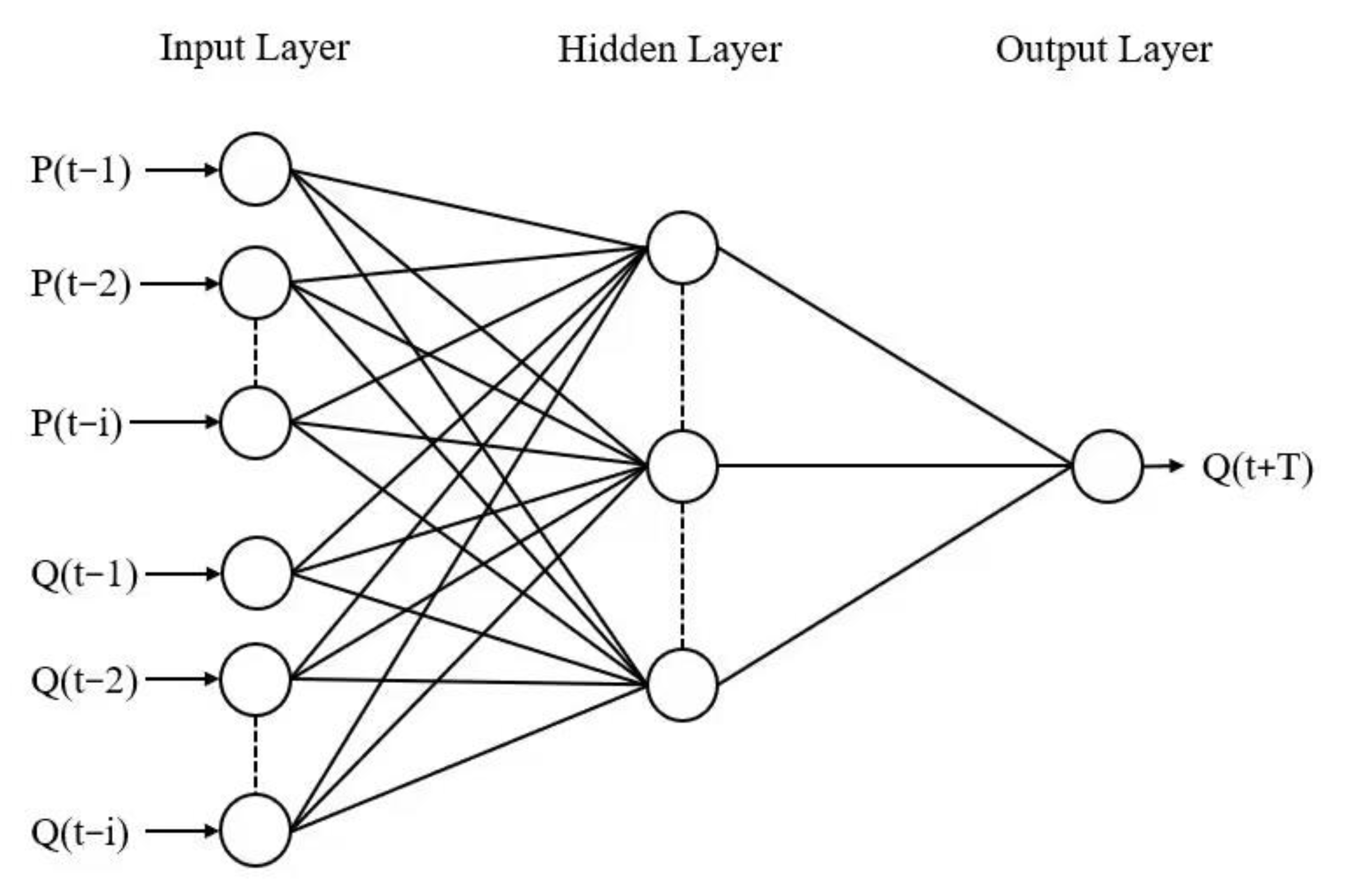
3.1.2. Standard Artificial Intelligence for Modeling

• BP Neural Network;

The BP neural network model, proposed by Rumelhart and McCelland, is capable of simultaneously learning and storing a large number of “input-output” mapping relationships, and is one of the most widely applied neural network models today [33]. Each node represents a function, and each connection between two nodes represents a weighted value of the signal they are connected to, called the weight, as shown in Figure 3. To reach the minimum, the specific form of back-propagation is as follows:

(1)

Error function definition

The error function is the layer-by-layer transfer of the function between the nodes in the hidden layer, after the training sample passes through the input layer, and the output layer passes through the output layer to obtain the sampling error after the corresponding error square function, $E_P$ [34]:

$$E_P=\frac{1}{2}{\displaystyle \sum }_{j=1}^m{(t_j^P-y_j^P)}^2$$

(7)

where $E_P$ is the sampling error, $t_j^P$ is the desired output, and $y_j^P$ is the actual output produced by the neural network on the input.

For $P_{ }$ samples, the global error is

$$E=\frac{1}{2}{\displaystyle \sum }_{P=1}^P{\displaystyle \sum }_{j=1}^m\left(t_j^P-y_j^P\right)={\displaystyle \sum }_{j=1}^m{E}_P$$

(8)

(2)

Output layer weight change

Using the cumulative error BP algorithm to adjust $w_{jk}$, lowering the global error E, i.e.,

$$\Delta w_{jk}=-\eta \frac{\partial E}{\partial w_{jk}}=-\eta \frac{\partial }{\partial w_{jk}}\left({\displaystyle \sum }_{P=1}^P{E}_p\right)={\displaystyle \sum }_{P=1}^P\left(-\eta \frac{\partial E_P}{\partial w_{jk}}\right)$$

(9)

where $\eta$ is the learning rate (%), and $w_{jk}$ is the output layer weight.

(3)

Implied weight change

$$\Delta v_{ki}=-\eta \frac{\partial E}{\partial v_{ki}}=-\eta \frac{\partial }{\partial v_{ki}}\left({\displaystyle \sum }_{P=1}^P{E}_p\right)={\displaystyle \sum }_{P=1}^P\left(-\eta \frac{\partial E_P}{\partial v_{ki}}\right)$$

(10)

where $v_{ki}$ is the implicit layer weight.

Define the error signal as

$${\delta }_{zk}=-\frac{\partial E_P}{\partial S_k}=-\frac{\partial E_P}{\partial z_k}·\frac{\partial z_k}{\partial S_k}$$

(11)

where $S_k$ is the bias from the previous layer to the current layer.

After the above formula processes, the final weight adjustment formula of the hidden layer neurons is

$$\Delta v_{ki}={\displaystyle \sum }_{P=1}^P{\displaystyle \sum }_{j=1}^m\eta \left(t_j^P-y_j^P\right)f_2^{\prime }\left(S_j\right)w_{jk}{f}_1^{\prime }\left(S_k\right)x_i$$

(12)

Figure 3. Structure of back-propagation (BP) neural networks.

Figure 3. Structure of back-propagation (BP) neural networks.

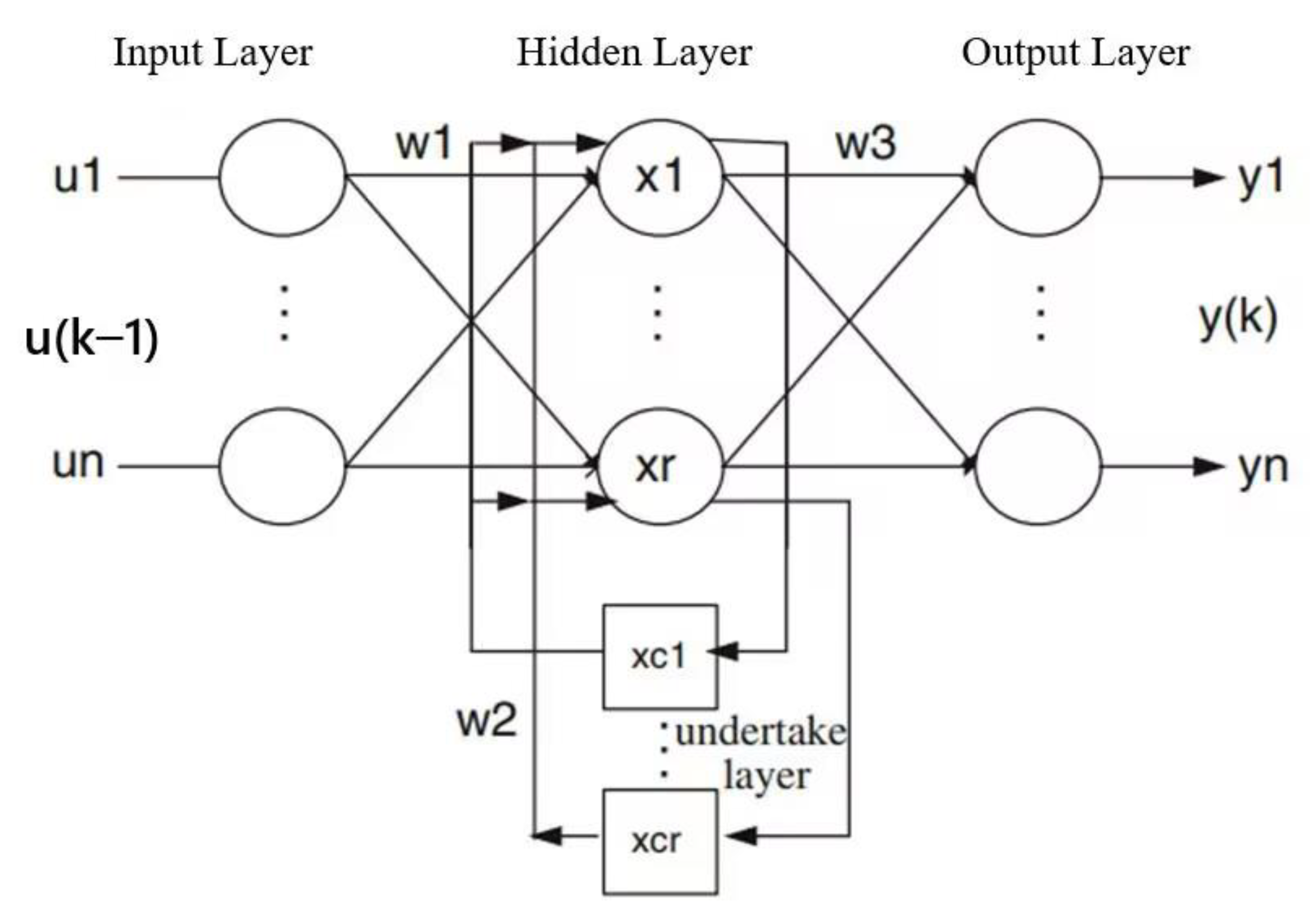
• Elman Neural Network;

The Elman neural network model is a class of local regression networks with extreme computational power, connecting local memory units with local feedback. Compared to the general static neural network, Elman has an additional association layer, which is used as the input of the implicit layer and as the input of the implicit layer at the previous moment, and has the characteristics of fast approximation and good dynamic characteristics [35]. The specific structure is shown in Figure 4 [36]. The mathematical model of the Elman neural network is

$$x_c\left(k\right)=\alpha ·x_c\left(k-1\right)+h\left(k-1\right)$$

(13)

where $x_c\left(k\right)$ is the take-up output at moment k and $\alpha$ is the feedback gain of the self-connection.

$$h\left(k\right)=f\left(w^{1}u\left(k-1\right)+w^3{x}_c\left(k\right)+b_h\right)$$

(14)

where $h\left(k\right)$ is the implied layer output value; and $w^1,$ $w^3$ are the connection weights from the input layer to the middle layer and the takeover layer to the middle layer, respectively.

$$y\left(k\right)=g\left(w^{2}h\left(k\right)+b_y\right)$$

(15)

where $g(\cdot )$ is the transfer function of the output neuron, and $w^2$ is the connection weight of the middle layer to the output layer.

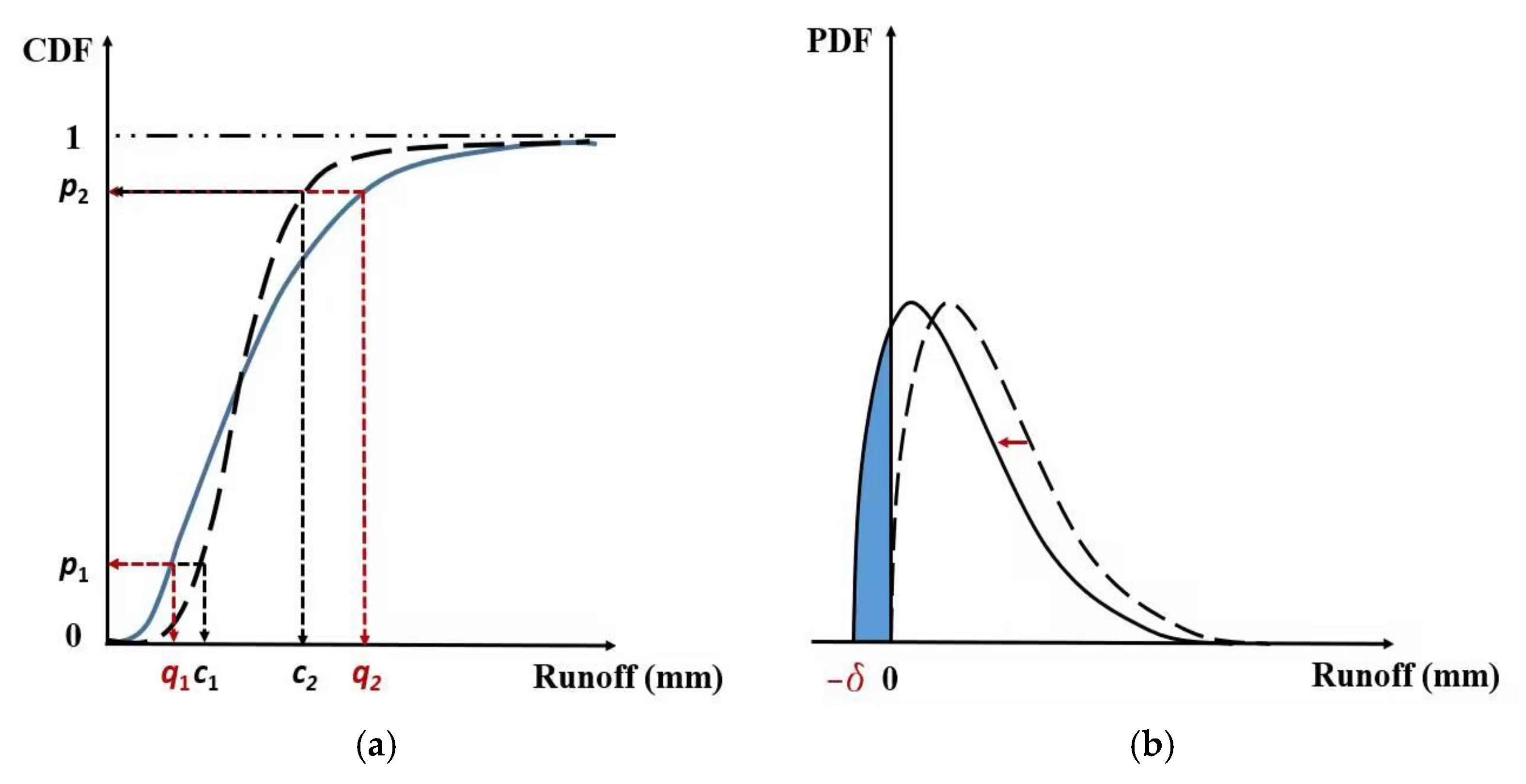
3.1.3. Quantile Mapping for Post-Processing

Quantile Mapping is a widely used bias-correction method. The statistical transformation process of the distribution-mapping method is to determine a statistical distribution in advance so that the distribution fitted by the observations is mapped to the distribution fitted by the predicted values by quantile with minimum error [37]. The method corrects the simulated runoff depth by establishing a transfer function between the simulated runoff depth and the observed runoff depth. The principle schematic of the quantum mapping method is shown in Figure 5, and the specific correction method is as follows: calculate the cumulative distribution function (CDF); construct the transfer function (TF); correct the model runoff depth for the validation period for each grid using the transfer function at the time of modeling; and obtain the correct results for the whole watershed [38].

3.2. Comparative Experimental Setup

3.2.1. Experimental Setup

First, the standard artificial intelligence models, namely, the BP neural network model and the Elman neural network model, were used for monthly runoff prediction. The prediction ability of the two AI models was initially investigated, and subsequent modeling was performed based on them. Secondly, the EMD and EEMD pre-processing techniques were combined with the two artificial intelligence models to construct the EMD–BP, the EEMD–BP, the EMD–Elman, and the EEMD–Elman models. The accuracy of these four models was evaluated, and the model with the best prediction outcomes was selected for subsequent study. Finally, the quantile mapping method was used to post-process the best prediction model from the previous step to see whether the prediction accuracy could be further improved.

3.2.2. Evaluation Metrics

The performance evaluation of a model by a single metric is usually limited [39], so we referred to the previous literature and synthetically selected four famous metrics for performance evaluation [27,40]. The Nash–Sutcliffe efficiency (NSE), the root mean square error (RMSE), the mean absolute percentage error (MAPE), and the peak percentage of threshold statistics (PPTS) were used to evaluate the prediction performance of the models. The NSE can evaluate the predictive capability of a model by measuring how close the simulated process values are to the observed values. The closer the value is to 1, the better the model performance. MAPE can assess the predictive accuracy of the smoothed component in the runoff series, with a value of 1 in the ideal case. RMSE is used to measure the variability of the data, and the smaller the value, the better the accuracy of the model [41]. To calculate the PPTS values, the original data samples are arranged in descending order and the predicted data samples are arranged in the same order. The parameter γ indicates a threshold, which can be chosen as 5% or 10%. The parameter G is the number of values above this threshold level. For example, PPTS (10) is the top 10% of flows or peak flows evaluated according to the PPTS criteria. A lower PPTS value indicates a more accurate peak flow prediction [42]. These four metrics are calculated as follows:

$$NSE=1-\frac{{{\displaystyle \sum }}_{i=1}^N{\left(y_i-y_i^{*}\right)}^2}{{{\displaystyle \sum }}_{i=1}^N{\left(y_i-\overline{y}\right)}^2}$$

(16)

$$RMSE=\sqrt{\frac{1}{n}{\displaystyle \sum }_{i=1}^N{(y_i^{-}-y_i^{*})}^2}$$

(17)

$$MAPE=\frac{1}{n}{\displaystyle \sum }_{i=1}^N\left|\frac{y_i-y_i^{*}}{y_i}\right|\times 100\%$$

(18)

$$PPTS\left(\gamma \right)=\frac{100}{\gamma }\frac{1}{n}{\displaystyle \sum }_{i=1}^G\left|\frac{y_i-y_i^{*}}{y_i}\right|\times 100\%$$

(19)

where $y_i$ is the measured value, $y_i^{*}$ is the simulated value, and $\overline{y}$ is the average of the measured values.

According to “Standard for Hydrological Information and Hydrological Forecasting” (GB/T22482-2008) [43], when NSE ≥ 0.90, the accuracy is set to Grade A; when 0.70 ≤ NSE < 0.90, the accuracy is Grade B; and when 0.50 ≤ NSE < 0.70, the accuracy is Grade C. If a forecast program’s accuracy reaches Grade A or B, it can be used to issue official forecasts; if a program’s accuracy only reaches Grade C, it can be used for reference forecasts but not official forecasts; and if a program’s accuracy is below Grade C, it can only be used for reference estimates.

4. Results and Analysis

4.1. Performance Investigation of Traditional Models

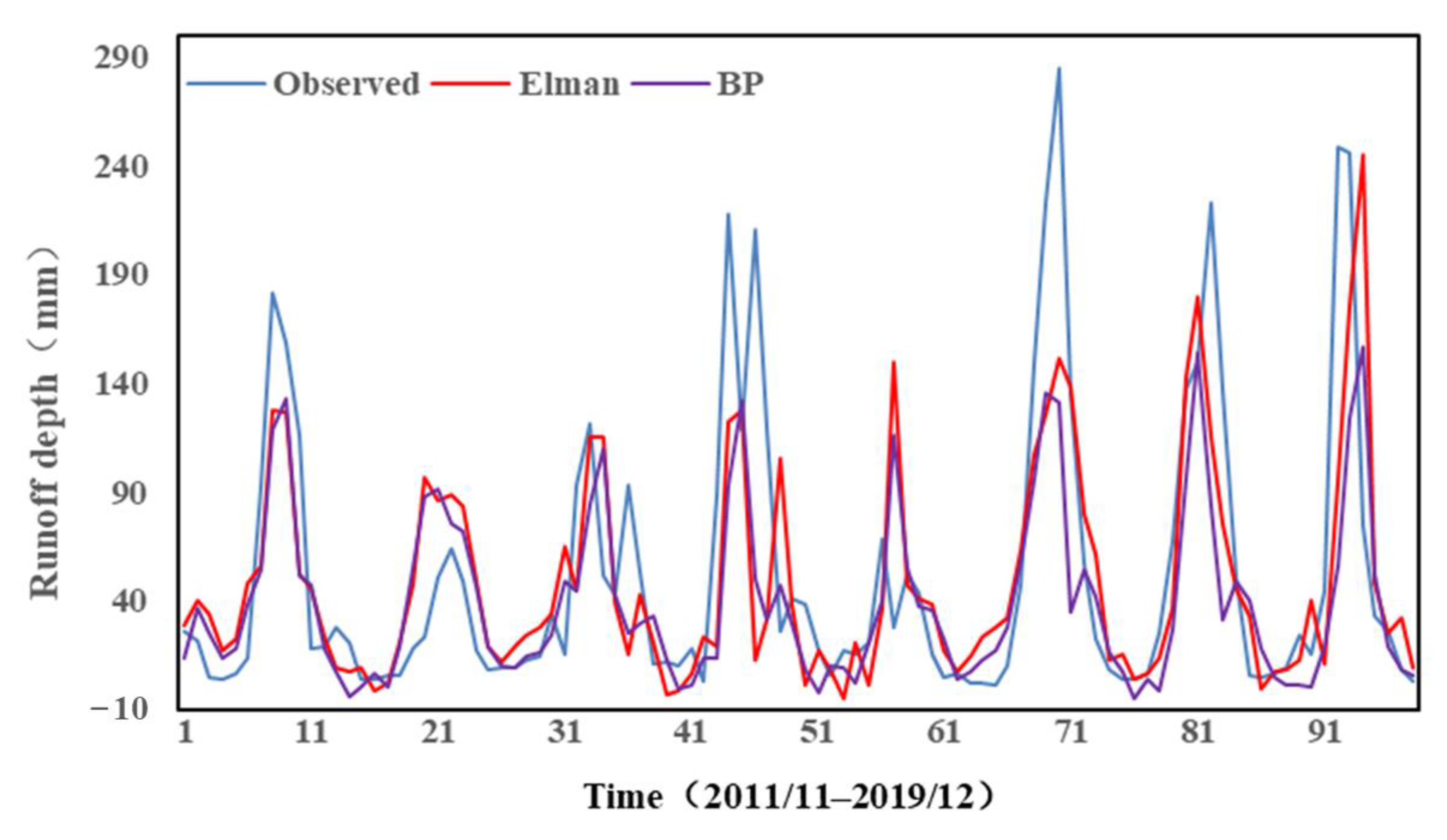
4.1.1. Results of Standard Artificial Intelligence Models

The prediction results obtained by two standard AI models are shown in Figure 6 and

Table 2. Evaluation of monthly runoff predictions by two standard AI models.

Model	NSE	MAPE (%)	RMSE (mm)	PPTS (10)
BP	0.49	83.35	45.46	4.69
Elman	0.43	108.36	50.00	4.37

.

The combined analysis shows that neither the BP nor the Elman model reached a prediction accuracy of Grade C or higher. In terms of the NSE evaluation index, the NSE value of the BP model was 0.49, while that of the Elman was 0.43. In terms of the MAPE evaluation index, the MAPE value of the BP model was 83.35%, while that of Elman model was 108.36%. In terms of the RMSE evaluation index, the RMSE value of the BP model was 45.46 mm, while that of the Elman model was 50.00 mm. In terms of the PPTS evaluation index, the PPTS value of the BP model was 4.69, while that of Elman model was 4.37. Taken together, the results indicate that the predictions of the BP model were better than those of the Elman model, but that overall neither model was satisfactory.

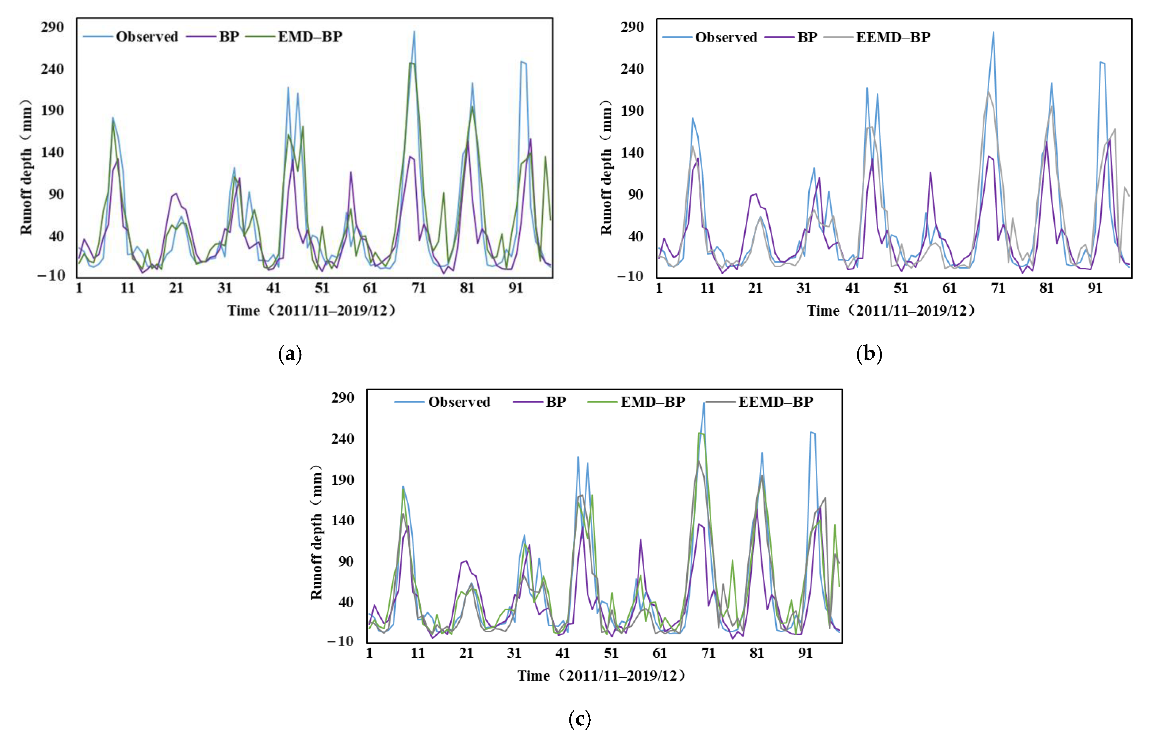
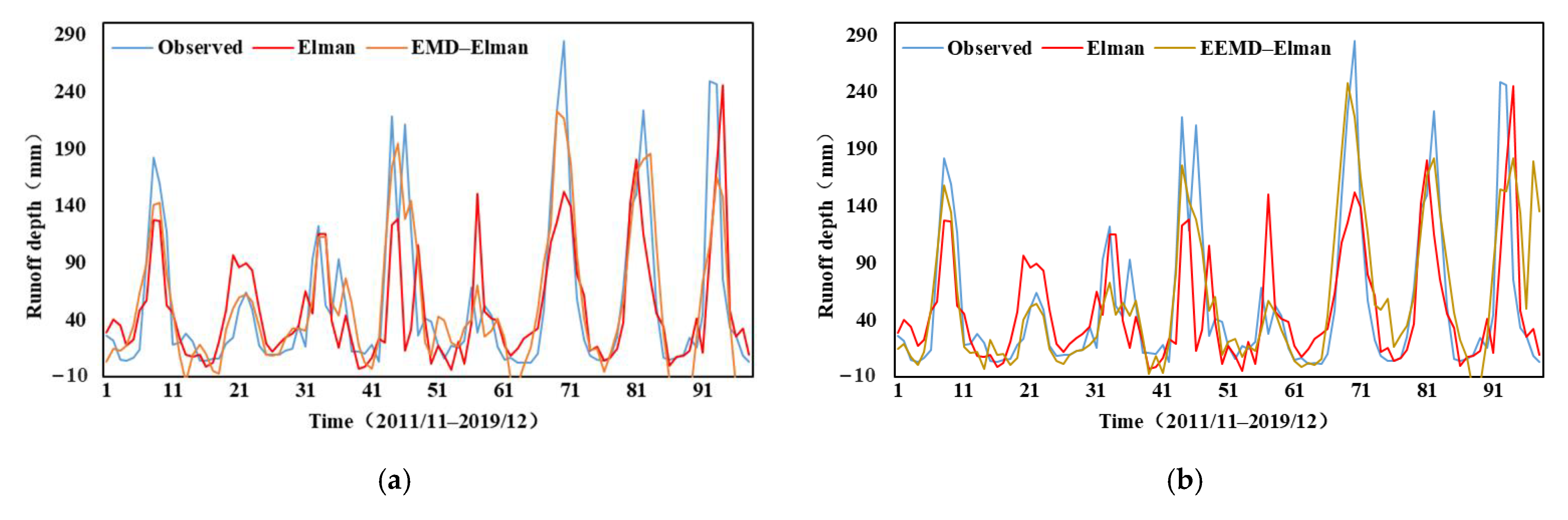
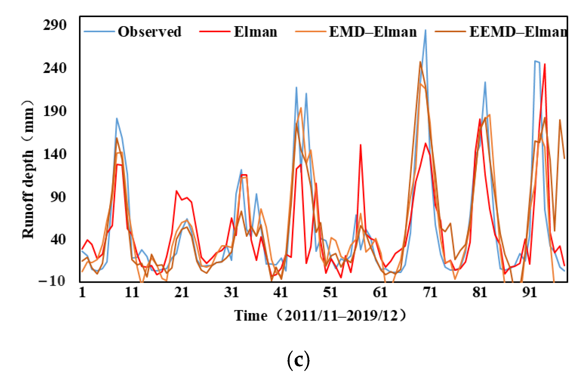
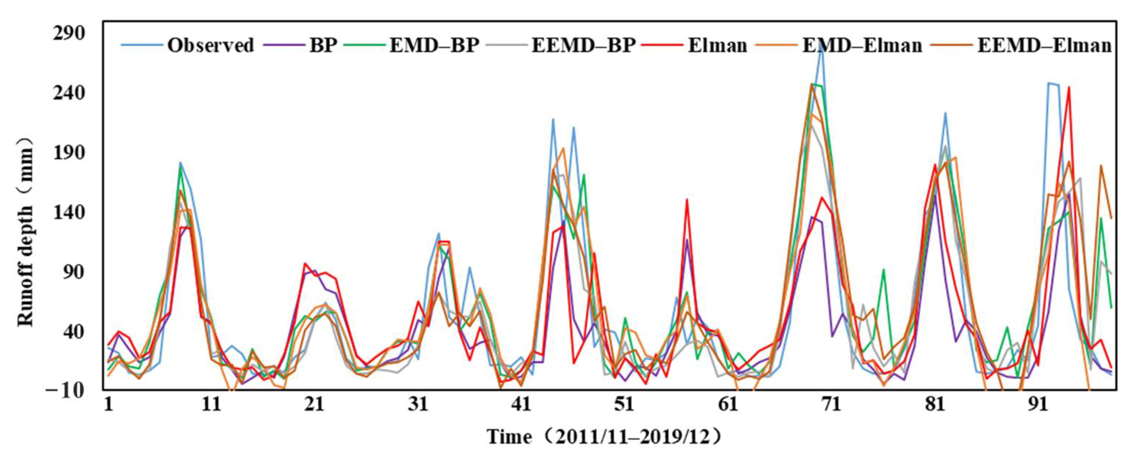
4.1.2. Results of Standard AI Models Combined with Pre-Processing Techniques

Given the limited prediction accuracy of the standard AI models, in this section, two preprocessing techniques with different characteristics and proven applications, EMD and EEMD, were combined with the standard AI models. First, each decomposition method was used to decompose the monthly runoff series of the validation set and to obtain the respective components. Second, the BP model and the Elman model were used to predict each component of each pre-processing decomposition, and the predicted components were summed to obtain the monthly runoff series. Finally, all the above prediction effects were compared and analyzed, and the best pre-processing-technique-based model was selected.

Four coupled models based on the pre-processing techniques and standard AI models were constructed: EMD–BP, EMD–Elman, EEMD–BP, and EEMD–Elman. The predictions of these four coupled models were compared with the standard BP and Elman models to evaluate the models’ performance and to determine the runoff prediction model with the best prediction results. Additionally, the original data and IMF component data were divided using the same training and validation sets. The division ratio was set to 8:2. The prediction results of the above four coupled models are shown in Figure 7, Figure 8 and Figure 9, and the index performance results of different coupled models are shown in

Table 3. Evaluation of double-coupled models’ monthly runoff predictions during the validation period.

Model	NSE	MAPE (%)	RMSE (mm)	PPTS (10)
BP	0.49	84.35	45.46	4.69
EMD–BP	0.71	160.74	34.32	2.39
EEMD–BP	0.70	117.01	36.08	2.51
Elman	0.43	108.36	50.00	4.37
EMD–Elman	0.72	138.53	42.76	2.40
EEMD–Elman	0.65	166.75	38.99	2.27

.

As seen in Figure 7 and Table 3, for the BP model, the coupling the model with pre-processing techniques showed better prediction results than the standard BP model alone. In terms of the NSE evaluation index, the NSE values of the EMD–BP and EEMD–BP models were 0.71 and 0.70, respectively. Compared with the BP model alone, the EMD–BP coupled model improved by 0.22, and the EEMD–BP coupled model improved by 0.21. The coupled prediction accuracies both reached Grade B, indicating a better model-fitting effect. In terms of the MAPE evaluation index, the two coupled models did not show a significant performance improvement compared with the BP model alone. In terms of the RMSE evaluation index, both coupled models improved compared with the unmodified model. The RMSE value of EMD–BP model was reduced by 25% compared to the BP model alone, while the RMSE value of the EEMD–BP model was reduced by about 21%. In terms of the PPTS evaluation index, the PPTS values of the EMD–BP and EEMD–BP models were 2.39 and 2.51, respectively. Compared with the unmodified BP model, the EMD–BP coupled model reduced its score by 2.30, and the EEMD–BP model reduced its score by 2.18. Therefore, both the EMD and EEMD pre-processing techniques improved the BP model’s prediction accuracy of the extreme values of runoff depth, and the EMD–BP model was better than the EEMD–BP model in terms of overall prediction.

As shown in Figure 8 and Table 3, for the Elman model, coupling the model with pre-processing techniques showed better prediction results than the standard Elman model alone. In terms of the NSE evaluation index, the NSE values of the EMD–Elman and EEMD–Elman models were 0.72 and 0.65, respectively, showing improvements of 0.29 and 0.22 compared with the unmodified Elman model. The prediction accuracy of the EMD–Elman coupled model reached Grade B, while that of the EEMD–Elman coupled model reached Grade C; thus, the EMD–Elman coupled model had better results. In terms of the MAPE evaluation index, neither the EMD–Elman model nor the EEMD–Elman model showed any obvious changes. In terms of the RMSE evaluation index, the RMSE value of the EMD–Elman model was reduced by 14% compared with the unmodified Elman model, while the RMSE value of the EEMD–Elman model was reduced by 22%; thus, the EEMD–Elman model performed better. In terms of the PPTS evaluation index, the PPTS values of the EMD–Elman and EEMD–Elman models were 2.40 and 2.27, respectively. Compared with the unmodified Elman model, the EMD–Elman coupled model reduced by 1.97, while the EEMD–Elman coupled model reduced by 2.10. In summary, it can be seen that applying pre-processing techniques improves the accuracy of the models’ predictions of extreme runoff volumes, and that EEMD outperforms EMD, indicating that the EEMD–Elman model can predict the extreme values better than other coupled models and that it is more advantageous in general.

Of the two models coupled with EMD, the EMD–Elman model had better prediction results with an NSE value of 0.72 and a prediction accuracy of Grade B. By contrast, the EMD–BP model had an NSE value of 0.71 and a prediction accuracy of Grade B. Of the two models coupled with EEMD, the EEMD–BP model had better prediction results, with an NSE value of 0.70 and a prediction accuracy of Grade B; the EEMD–Elman model had an NSE value of 0.65 and a prediction accuracy of Grade C. Overall, of the two pre-processing techniques, the models coupled with EMD had better prediction results than the corresponding models coupled with EEMD, as the EMD-coupled models both had higher NSE index scores and prediction accuracies of Grade B. Taken together, the EMD–Elman model is the best model among the four models, with an NSE value of 0.72 and a prediction accuracy of Grade B.

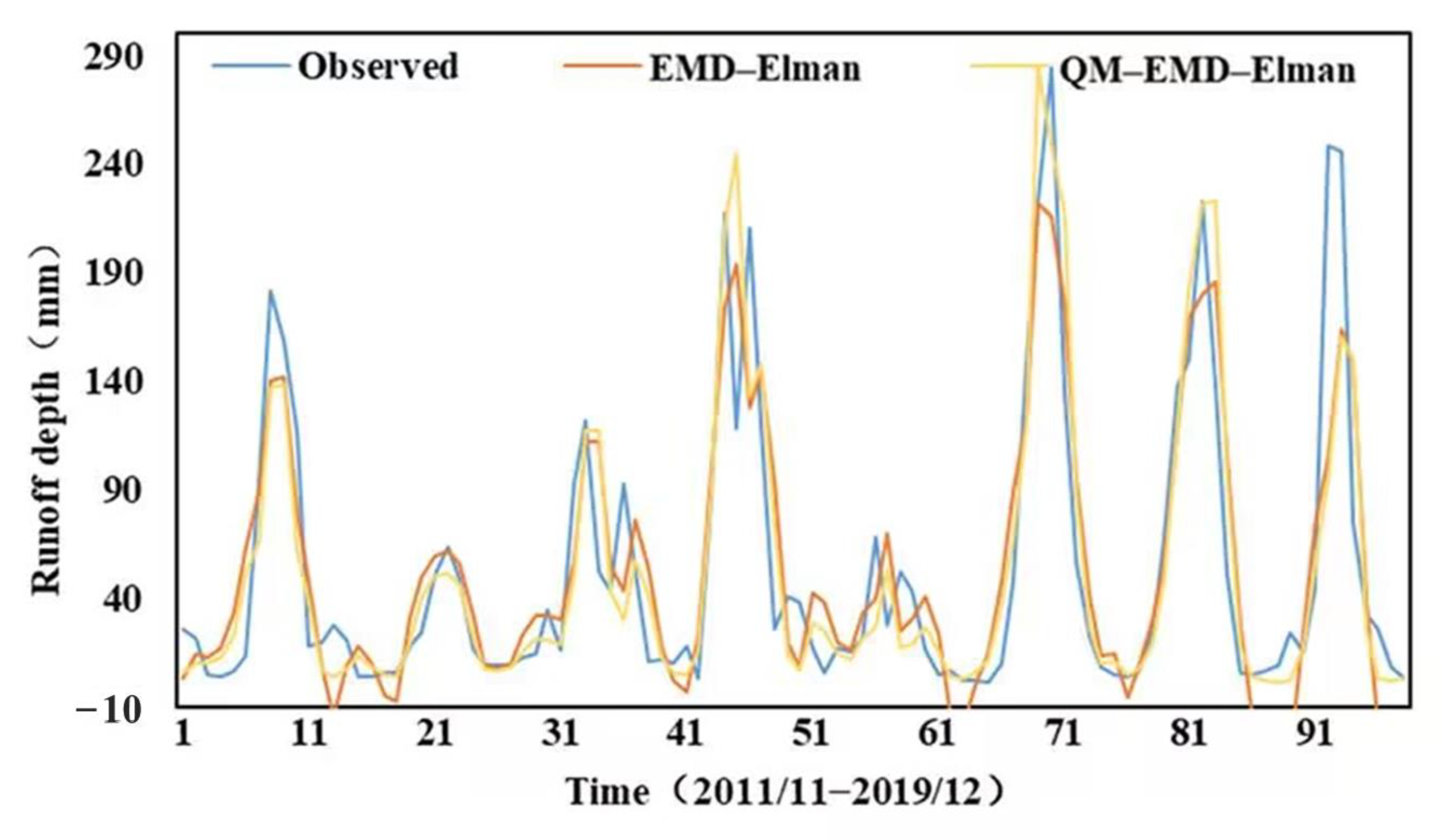
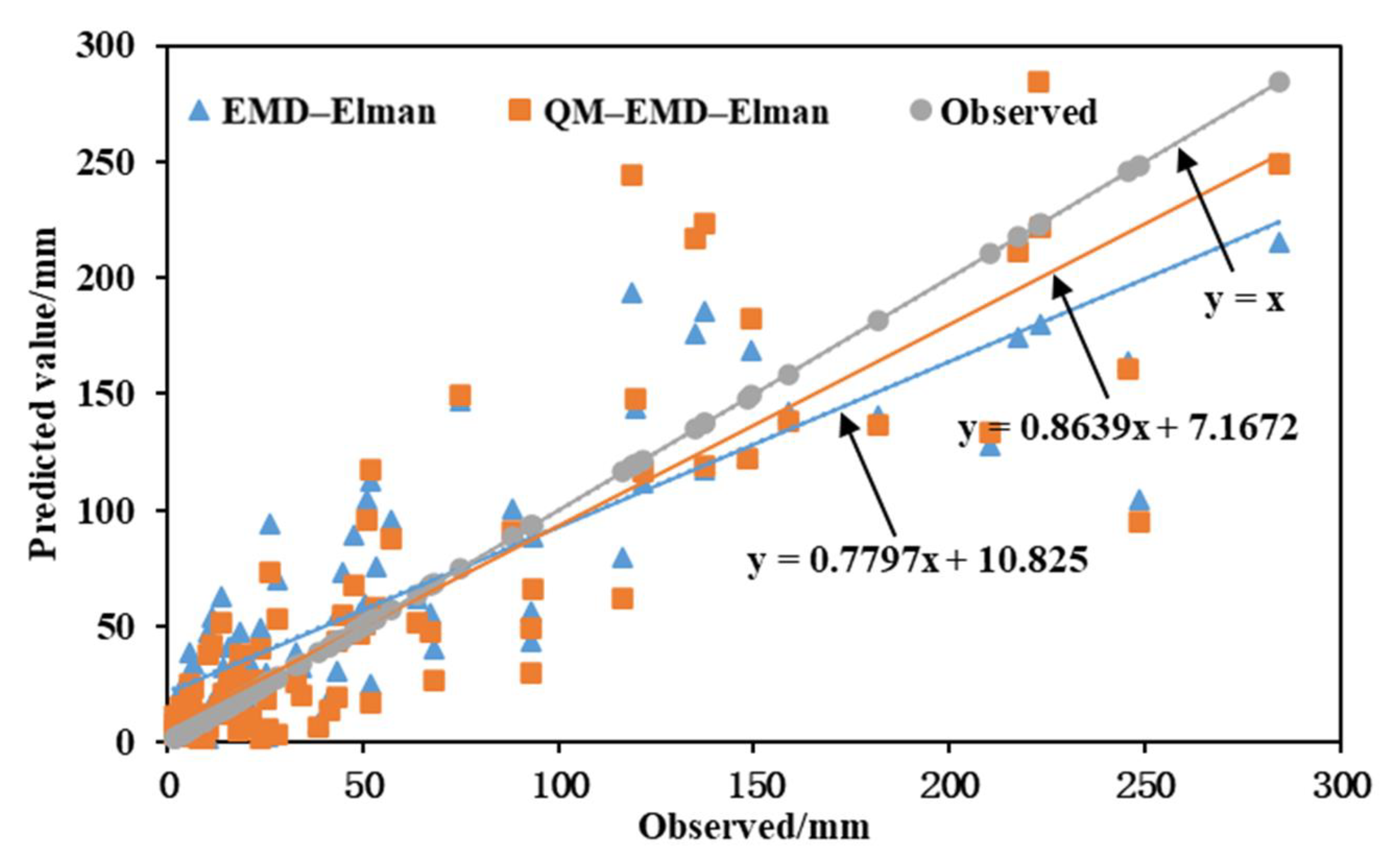
4.2. Performance Investigation of Standard AI Models Combined with Pre-Processing Techniques and Post-Processing Methods

In the previous section, based on the prediction results of the traditional models coupled with pre-processing techniques, it was determined that the EMD–Elman model had the best predictive capacity with an NSE value of 0.72 and a prediction accuracy of Grade B. In this section, the QM–EMD–Elman model is formed using the quantile mapping method coupled with the selected EMD–Elman model. The prediction results are shown in Figure 10, and the evaluation of the result indicators is shown in

Table 4. Evaluation of triple-coupled model’s monthly runoff predictions during the validation period.

Model	NSE	MAPE (%)	RMSE (mm)	PPTS (10)
EMD–Elman	0.72	138.53	42.76	2.40
QM–EMD–Elman	0.73	74.57	34.60	2.36

.

From Table 4 and Figure 10, it can be seen that the NSE value of the QM–EMD–Elman model is 0.73, which is an improvement of 0.01 compared to the EMD–Elman model, with a prediction accuracy of Grade B. Meanwhile, the MAPE value is 74.57%, which is 63.96% lower than that of the EMD–Elman model. The RMSE value is 34.60, which is 8.16 lower than that of the EMD–Elman model. The PPTS value is 2.36, which is 0.04 lower than that of the EMD–Elman model. Thus, the QM–EMD–Elman model shows a significant improvement in MAPE and RMSE metrics, with little fluctuation in NSE and PPTS metrics.

As can be seen from Figure 11, the plot is a scatter fit of the two models mentioned above. By comparing each model with the linear trend line of the line y = x, it is clear that the linear trend line of the QM–EMD–Elman model is closest to the line y = x, while the EMD–Elman model is the following closest. This shows that the QM–EMD–Elman model has better prediction accuracy than the other model.

In Figure 12, the NSE indicator is analyzed separately because it is the indicator that best reflects a model’s strengths and weaknesses [44]. As can be seen in the figure, the NSE indicators of the Elman model, EMD–Elman model, and QM–EMD–Elman model show an increasing trend, and it can also be seen that the QM–EMD–Elman model has the best prediction results among the three models.

As can be seen from Figure 13, the prediction accuracy of the Elman model, the EMD–Elman model, and the QM–EMD–Elman model was further evaluated using Taylor plots. Taylor diagrams are based on the geometrical relationships between the correlation coefficient, standard deviation, and the root mean square error [17]. Taylor plots precisely and effectively reflect the properties of a prediction model, indicating when results are closer to the observed values, and are thus better prediction [45]. The graph shows that the predicted values of the QM–EMD–Elman model are closest to the observed values.

5. Discussion

Roughly 9% of the global population partly or fully relies on karst water resources [46], making the prediction of runoff in karst areas an issue of significant engineering and scientific importance. However, the complex and unique topography of karst regions leads to difficulties for traditional hydrological models trying to accurately generalize and predict its behavior, especially when the underlying physical relationships (or underground geographical characteristics) cannot be explicitly obtained. The development of standard AI models, pre-processing techniques, and post-processing methods have provided new opportunities to improve the accuracy of runoff prediction in karst areas, but they have only been only partially explored. The present study helps to bridge this gap in knowledge by investigating the predictive performance of standard AI models, AI models coupled with pre-processing techniques, and AI models coupled with both pre-processing techniques and quantile mapping post-processing methods. We now further discuss the similarities and differences between these models, as well as policy recommendations, innovations, limitations, and further research.

5.1. Similarities and Differences

The prediction results of the standard AI models show that BP performs better than Elman, which is consistent with the results of previous studies. In a study of the hydrology field, Liu et al. [47] studied the flood prediction power of the model in the Longquan Creek watershed. The results showed that the BP model and the Elman model provided the best and the worst performance, respectively, for flood prediction in Longquan basin under the same prediction lead time. The BP model has also demonstrated more accurate predictions than the Elman model in other fields, such as power system protection and control. The outcome of the research conducted by Liu et al. shows that the starting criteria for a fault-recorder algorithm based on the BP neural network can effectively complete the recording start, with minor prediction error [48]. In each of these studies, BP showed better predictions than Elman.

After coupling the EMD and EEMD pre-processing techniques with the standard AI models to form double-coupled models, the predictions were significantly better than from the unmodified models. Similar results were also found by Zhao et al. [49]. They compared the performance of the constructed EEMD–AR model, EMD–AR model, and unmodified AR model using runoff data from four hydrological stations in the upper Fen River basin, China. The results showed that the hybrid EEMD–AR model was more accurate in predicting runoff. This phenomenon may be caused by the fact that the data pre-processing technique transforms the original series into multiple relatively stationary series, and thus can effectively reduce the impact of the nonlinear and nonstationary characteristics. Therefore, when making runoff predictions, preprocessing can be performed on the runoff series to fully exploit the limited sample data and extract meaningful information reflecting changes in the series, and then coupled with a single model, thus improving the accuracy of runoff prediction.

Ensemble empirical modal decomposition can better solve the modal confounding problem in the empirical modal decomposition method by taking advantage of the good zero-mean characteristic of white noise. Li et al. [18] proposed the EMD–ANN and the EEMD–ANN models for long-term runoff prediction and evaluated the prediction accuracy of both; they found that, compared with the EMD–ANN model, the EEMD–ANN model performed better in predicting high flow values, and best matched the observed results. In the present study, the coupled models formed by EMD with Elman and BP were more accurate than the coupled models formed by EEMD with Elman and BP, which is inconsistent with some scholars’ studies [18,50]. This phenomenon may be due to the fact that the runoff series in the present study are based on karst areas, where the subterranean topographical conditions are extremely different from other areas, and which have a continuous effect on runoff [17].

Among three of the evaluation indicators employed in the present study, better model simulation is indicated by higher values for the Nash–Sutcliffe efficiency, and lower values for the root mean square error and the mean absolute percentage error [51]. The prediction results of the QM–EMD–Elman model showed a significant improvement in the MAPE and RMSE indicators compared with the EMD–Elman model, with only a slight fluctuation in the NSE indicator. This indicates that the prediction accuracy of the triple-coupled model, formed by adding post-processing to the double-coupled model, was improved again, suggesting that the post-processing method can effectively control the prediction error. This result is consistent with the study conducted by Jin et al. [52] In this study, Jin used the Xinanjiang model driven by seven control forecast products, such as ECMWF and UKMO, for integrated runoff prediction and then investigated the effects of data processing schemes on runoff prediction accuracy and uncertainty, using the post-processing method of the BMA model. The results showed that post-processing methods are essential to improve the accuracy and rationality of meteorological and hydrological runoff predictions. This phenomenon may be because the post-processing method removes the negative values from the prediction results and ensures that all data are positive, which controls the output error very well. Since the ensemble model can combine the advantages of several single models, the ensemble model performs better for runoff forecasting. Therefore, the QM–EMD–Elman model can significantly improve the precision of monthly runoff predictions, and its runoff series prediction results are meaningful.

5.2. Policy Recommendations

Runoff prediction methods with higher accuracy are urgently needed in karst basins to provide data support and theoretical support for reservoir runoff forecasting work and efficient water resources management. The above studies show that standard AI models can be effectively applied to runoff prediction, and that adding pre-processing techniques and post-processing methods can further improve prediction accuracy. Water resource managers can choose different combinations of standard AI models, pre-processing techniques, and post-processing methods for runoff prediction to select the best runoff prediction model for more scientific and effective water resource management, given the actual situation of the basin.

5.3. Innovation, Limitations, and Further Research

In this paper, the performance of the coupled model formed by standard artificial intelligence models, pre-processing techniques, and the quantile mapping post-processing method was evaluated. The QM–EMD–Elman model for monthly runoff prediction in the karst areas was constructed. The EMD pre-processing technique can be used to generate a smooth series, which effectively reduces the effects of non-linearity and non-stationarity in the original series. Additionally, the QM post-processing method can be used to remove the negative values from the prediction results, which can effectively control the output errors. The proposed QM–EMD–Elman model was more effective in capturing the runoff influence patterns, and can be used for monthly runoff predictions in karst areas.

The restricted information limits the research process, and the study of runoff prediction can be further improved in the following aspects in future research.

Due to the data, the conclusions and results of this study have limited portability and may not be directly transferred to other watersheds.

The pre-processing technique used in the study divides the data into high-frequency components, low-frequency components, and trend terms by frequency. Then the different components were uniformly studied for prediction using the same model, and the results were summed afterward [53]. In future studies, different models can be used to predict different frequency components to find the best model for each component.

Changes in runoff have become more complex due to the effects of climate change and human activities. Nevertheless, artificial intelligence models cannot adequately consider these two factors to predict runoff. Therefore, there is a need to further study how models can fully integrate factors such as climate and human activity.

6. Conclusions

In this paper, based on the monthly runoff data for the Chengbi River basin, spanning a total period of 492 months from 1979–2019, we aimed to investigate the predictive performance of standard AI models, AI models coupled with pre-processing techniques, and AI models coupled with both pre-processing techniques and quantile mapping post-processing methods. The primary conclusions obtained from this study are as follows.

The monthly runoff of the watershed was predicted based on standard artificial intelligence models, namely, the BP Elman models. The results showed that the BP model predicted better than the Elman model, but that the overall prediction accuracy of both models was poor.

Four models based on Empirical Modal Decomposition and Ensemble Empirical Modal Decomposition, each coupled with the two standard artificial intelligence models, were constructed to predict monthly runoff in the watershed. The results showed that pre-processing techniques can improve the accuracy of runoff prediction. On the two pre-processing techniques used in this study, EMD produced better predictions and higher NSE values than EEMD, and the EMD–Elman model was the best double-coupled model of the four that were tested.

A QM–EMD–Elman triple-coupled model based on the quantile mapping (QM) method, coupled with the EMD–Elman double-coupled model, was constructed to predict monthly runoff in the watershed. The results showed that the QM–EMD–Elman model had improved prediction results, and that the post-processing method improved the accuracy of runoff prediction. The triple-coupled approach of pre-processing techniques, standard artificial intelligence models, and post-processing methods is an effective method for monthly runoff prediction in karst areas.

References

1. Sterling, S.M.; Ducharne, A.; Polcher, J. The impact of global land-cover change on the terrestrial water cycle. Nat. Clim. Chang. 2013, 3, 385–390. [Google Scholar] [CrossRef]
2. Yuan, X.; Ji, B.; Zhang, S.; Tian, H.; Chen, Z. An improved artificial physical optimization algorithm for dynamic dispatch of generators with valve-point effects and wind power. Energy Convers. Manag. 2014, 82, 92–105. [Google Scholar] [CrossRef]
3. Li, L.; Tan, X. Big-Data-Driven Intelligent Wireless Network and Use Cases. In Proceedings of the IEEE International Conference on Communications (ICC), Online, 14–23 June 2021. [Google Scholar]
4. Hunt, K.M.R.; Matthews, G.R.; Pappenberger, F.; Prudhomme, C. Using a long short-term memory (LSTM) neural network to boost river streamflow forecasts over the western United States. Hydrol. Earth Syst. Sci. 2022, 26, 5449–5472. [Google Scholar] [CrossRef]
5. Sharifi, A.; Dinpashoh, Y.; Mirabbasi, R. Daily runoff prediction using the linear and non-linear models. Water Sci. Technol. 2017, 76, 793–805. [Google Scholar] [CrossRef] [PubMed]
6. Li, C.; Zhu, L.; He, Z.; Gao, H.; Yang, Y.; Yao, D.; Qu, X. Runoff Prediction Method Based on Adaptive Elman Neural Network. Water 2019, 11, 1113. [Google Scholar] [CrossRef] [Green Version]
7. Peng, T.; Zhou, J.; Zhang, C.; Fu, W. Streamflow Forecasting Using Empirical Wavelet Transform and Artificial Neural Networks. Water 2017, 9, 406. [Google Scholar] [CrossRef] [Green Version]
8. Yuan, X.; Chen, C.; Lei, X.; Yuan, Y.; Adnan, R.M. Monthly runoff forecasting based on LSTM–ALO model. Stoch. Environ. Res. Risk Assess. 2018, 32, 2199–2212. [Google Scholar] [CrossRef]
9. Qu, B.; Zhang, X.; Pappenberger, F.; Zhang, T.; Fang, Y. Multi-Model Grand Ensemble Hydrologic Forecasting in the Fu River Basin Using Bayesian Model Averaging. Water 2017, 9, 74. [Google Scholar] [CrossRef]
10. Bogner, K.; Liechti, K.; Zappa, M. Post-Processing of Stream Flows in Switzerland with an Emphasis on Low Flows and Floods. Water 2016, 8, 115. [Google Scholar] [CrossRef] [Green Version]
11. Hartmann, A.; Goldscheider, N.; Wagener, T.; Lange, J.; Weiler, M. Karst water resources in a changing world: Review of hydrological modeling approaches. Rev. Geophys. 2014, 52, 218–242. [Google Scholar] [CrossRef]
12. Zhou, Q.; Chen, L.; Singh, V.P.; Zhou, J.; Chen, X.; Xiong, L. Rainfall-runoff simulation in karst dominated areas based on a coupled conceptual hydrological model. J. Hydrol. 2019, 573, 524–533. [Google Scholar] [CrossRef]
13. Niu, W.-J.; Feng, Z.-K. Evaluating the performances of several artificial intelligence methods in forecasting daily streamflow time series for sustainable water resources management. Sustain. Cities Soc. 2021, 64, 102562. [Google Scholar] [CrossRef]
14. Meng, X.; Yin, M.; Ning, L.; Liu, D.; Xue, X. A threshold artificial neural network model for improving runoff prediction in a karst watershed. Environ. Earth Sci. 2015, 74, 5039–5048. [Google Scholar] [CrossRef]
15. An, L.; Hao, Y.; Yeh, T.-C.J.; Liu, Y.; Liu, W.; Zhang, B. Simulation of karst spring discharge using a combination of time–frequency analysis methods and long short-term memory neural networks. J. Hydrol. 2020, 589, 125320. [Google Scholar] [CrossRef]
16. Siou, L.K.A.; Johannet, A.; Borrell, V.; Pistre, S. Complexity selection of a neural network model for karst flood forecasting: The case of the Lez Basin (southern France). J. Hydrol. 2011, 403, 367–380. [Google Scholar] [CrossRef] [Green Version]
17. Mo, C.; Liu, G.; Lei, X.; Zhang, M.; Ruan, Y.; Lai, S.; Xing, Z. Study on the Optimization and Stability of Machine Learning Runoff Prediction Models in the Karst Area. Appl. Sci. 2022, 12, 4979. [Google Scholar] [CrossRef]
18. Zhao, Y.; Liao, W.; Lei, X. Hydrological Simulation for Karst Mountain Areas: A Case Study of Central Guizhou Province. Water 2019, 11, 991. [Google Scholar] [CrossRef] [Green Version]
19. Fleury, P.; Plagnes, V.; Bakalowicz, M. Modelling of the functioning of karst aquifers with a reservoir model: Application to Fontaine de Vaucluse (South of France). J. Hydrol. 2007, 345, 38–49. [Google Scholar] [CrossRef]
20. Palanisamy, B.; Workman, S.R. Hydrologic Modeling of Flow through Sinkholes Located in Streambeds of Cane Run Stream, Kentucky. J. Hydrol. Eng. 2015, 20, 04014066. [Google Scholar] [CrossRef]
21. Nikolaidis, N.; Bouraoui, F.; Bidoglio, G. Hydrologic and geochemical modeling of a karstic Mediterranean watershed. J. Hydrol. 2013, 477, 129–138. [Google Scholar] [CrossRef]
22. Sun, S.; Deng, H.; Wang, Q. Simulation and comparative study of two types of Topographic Index model for a homogeneous mountain catchment. Sci. China Earth Sci. 2014, 57, 2089–2099. [Google Scholar] [CrossRef]
23. Campbell, C.; Sullivan, S.M. Simulating time-varying cave flow and water levels using the Storm Water Management Model. Eng. Geol. 2002, 65, 133–139. [Google Scholar] [CrossRef]
24. Dvory, N.Z.; Ronen, A.; Livshitz, Y.; Adar, E.; Kuznetsov, M.; Yakirevich, A. Quantification of Groundwater Recharge from an Ephemeral Stream into a Mountainous Karst Aquifer. Water 2018, 10, 79. [Google Scholar] [CrossRef] [Green Version]
25. Mo, C.; Ruan, Y.; Xiao, X.; Lan, H.; Jin, J. Impact of climate change and human activities on the baseflow in a typical karst basin, Southwest China. Ecol. Indic. 2021, 126, 107628. [Google Scholar] [CrossRef]
26. Feng, Z.-K.; Niu, W.-J.; Tang, Z.-Y.; Jiang, Z.-Q.; Xu, Y.; Liu, Y.; Zhang, H.-R. Monthly runoff time series prediction by variational mode decomposition and support vector machine based on quantum-behaved particle swarm optimization. J. Hydrol. 2020, 583, 124627. [Google Scholar] [CrossRef]
27. Meng, E.; Huang, S.; Huang, Q.; Fang, W.; Wu, L.; Wang, L. A robust method for non-stationary streamflow prediction based on improved EMD-SVM model. J. Hydrol. 2018, 568, 462–478. [Google Scholar] [CrossRef]
28. Huang, N.E.; Shen, Z.; Long, S.R.; Wu, M.C.; Shih, H.H.; Zheng, Q.; Yen, N.-C.; Tung, C.C.; Liu, H.H. The empirical mode decomposition and the Hilbert spectrum for nonlinear and non-stationary time series analysis. Proc. R. Soc. Lond. Ser. A Math. Phys. Eng. Sci. 1998, 454, 903–995. [Google Scholar] [CrossRef]
29. Chang, M.P.J.L.; Roura, E.A.; Font, C.O.; Gilbreath, C.; Oh, E. Applying the Hilbert-Huang decomposition to horizontal light propagation Cn2 data. In Proceedings of the Conference on Advances in Stellar Interferometry, Orlando, FL, USA, 25–30 May 2006. [Google Scholar] [CrossRef] [Green Version]
30. Feng, Z.-K.; Niu, W.-J.; Wan, X.-Y.; Xu, B.; Zhu, F.-L.; Chen, J. Hydrological time series forecasting via signal decomposition and twin support vector machine using cooperation search algorithm for parameter identification. J. Hydrol. 2022, 612, 128213. [Google Scholar] [CrossRef]
31. Zheng, J.; Cheng, J.; Yang, Y. Partly Ensemble Local Characteristic-Scale Decomposition: A New Noise Assisted Data Analysis Method. Acta Electron. Sin. 2013, 41, 1030–1035. [Google Scholar]
32. Wang, W.-C.; Chau, K.-W.; Xu, D.-M.; Chen, X.-Y. Improving Forecasting Accuracy of Annual Runoff Time Series Using ARIMA Based on EEMD Decomposition. Water Resour. Manag. 2015, 29, 2655–2675. [Google Scholar] [CrossRef]
33. McClelland, J.L.; Rumelhart, D.E. Distributed memory and the representation of general and specific information. J. Exp. Psychol. Gen. 1985, 114, 159–197. [Google Scholar] [CrossRef] [PubMed]
34. Cui, D. Application of Hidden Multilayer BP Neural Network Model in Runoff Prediction. Hydrology 2013, 33, 68–73. [Google Scholar]
35. Cheng, Y.-C.; Qi, W.-M.; Zhao, J. A New Elman Neural Network and Its Dynamic Properties. In Proceedings of the IEEE International Conference on Cybernetic Intelligent Systems (CIS 2008), Chengdu, China, 21–24 September 2008; pp. 261–265. [Google Scholar]
36. Ding, S.; Zhang, Y.; Chen, J.; Jia, W. Research on using genetic algorithms to optimize Elman neural networks. Neural Comput. Appl. 2012, 23, 293–297. [Google Scholar] [CrossRef]
37. Guo, Q.; Chen, J.; Zhang, X.; Shen, M.; Chen, H.; Guo, S. A new two-stage multivariate quantile mapping method for bias correcting climate model outputs. Clim. Dyn. 2019, 53, 3603–3623. [Google Scholar] [CrossRef]
38. Cannon, A.J.; Sobie, S.R.; Murdock, T.Q. Bias Correction of GCM Precipitation by Quantile Mapping: How Well Do Methods Preserve Changes in Quantiles and Extremes? J. Clim. 2015, 28, 6938–6959. [Google Scholar] [CrossRef]
39. Knoben, W.J.M.; Freer, J.E.; Woods, R.A. Technical note: Inherent benchmark or not? Comparing Nash–Sutcliffe and Kling–Gupta efficiency scores. Hydrol. Earth Syst. Sci. 2019, 23, 4323–4331. [Google Scholar] [CrossRef] [Green Version]
40. Zuo, G.; Luo, J.; Wang, N.; Lian, Y.; He, X. Decomposition ensemble model based on variational mode decomposition and long short-term memory for streamflow forecasting. J. Hydrol. 2020, 585, 124776. [Google Scholar] [CrossRef]
41. Yue, Z.; Ai, P.; Xiong, C.; Song, Y.; Hong, M.; Yu, J. Mid- and long-term runoff forecasting based on improved deep belief networks model. J. Hydroelectr. Eng. 2020, 39, 33–46. [Google Scholar]
42. Zuo, G.; Luo, J.; Wang, N.; Lian, Y.; He, X. Two-stage variational mode decomposition and support vector regression for streamflow forecasting. Hydrol. Earth Syst. Sci. 2020, 24, 5491–5518. [Google Scholar] [CrossRef]
43. GB/T 22482-2008; Standard for Hydrological Information and Hydrological Forecasting. Standardization Administration of China: Beijing, China, 2008; p. 16.
44. He, R.-R.; Chen, Y.; Huang, Q.; Pan, Z.-W.; Liu, Y. Predictability of Monthly Streamflow Time Series and its Relationship with Basin Characteristics: An Empirical Study Based on the MOPEX Basins. Water Resour. Manag. 2020, 34, 4991–5007. [Google Scholar] [CrossRef]
45. Sapankevych, N.I.; Sankar, R. Time Series Prediction Using Support Vector Machines: A Survey. IEEE Comput. Intell. Mag. 2009, 4, 24–38. [Google Scholar] [CrossRef]
46. Stevanović, Z. Karst waters in potable water supply: A global scale overview. Environ. Earth Sci. 2019, 78, 662. [Google Scholar] [CrossRef]
47. Liu, D.; Ge, L.; Xu, Y.; Zhang, S.; Chiang, Y. Flood prediction by multi-hydrological models with forecasting ability analysis. J. Zhejiang Univ. Eng. Sci. 2021, 55, 1010–1018. [Google Scholar]
48. Liu, J.; Li, T.; Fu, J.; Wu, N. Criteria algorithm for smart substation recorder starting based on BP & Elman neural network. Power Syst. Prot. Control 2014, 42, 110–115. [Google Scholar]
49. Zhao, X.-H.; Chen, X. Auto Regressive and Ensemble Empirical Mode Decomposition Hybrid Model for Annual Runoff Forecasting. Water Resour. Manag. 2015, 29, 2913–2926. [Google Scholar] [CrossRef]
50. Sibtain, M.; Li, X.; Bashir, H.; Azam, M.I. A Hybrid Model for Runoff Prediction Using Variational Mode Decomposition and Artificial Neural Network. Water Resour. 2021, 48, 701–712. [Google Scholar] [CrossRef]
51. Parvaze, S.; Khan, J.N.; Kumar, R.; Allaie, S.P. Temporal flood forecasting for trans-boundary Jhelum River of Greater Himalayas. Arch. Meteorol. Geophys. Bioclimatol. Ser. B 2021, 144, 493–506. [Google Scholar] [CrossRef]
52. Jin, J.; Shu, Z.; Chen, M.; Wang, G.; Sun, Z.; He, R. Meteo-hydrological coupled runoff forecasting based on numerical weather prediction products. Adv. Water Sci. 2019, 30, 316–325. [Google Scholar]
53. Chitsaz, N.; Azarnivand, A.; Araghinejad, S. Pre-processing of data-driven river flow forecasting models by singular value decomposition (SVD) technique. Hydrol. Sci. J. 2016, 61, 2164–2178. [Google Scholar] [CrossRef]
Figure 1. The approximate locations of the Chengbi River Karst Basin.
Applsci 13 00088 g001
Figure 2. Flowchart of the research in this study.
Applsci 13 00088 g002
Figure 4. Schematic diagram of Elman model structure.
Applsci 13 00088 g004
Figure 5. Principle of the quantile mapping method. (a) Cumulative distribution function. (b) Probability density function.
Applsci 13 00088 g005
Figure 6. Forecasted and observed monthly streamflow during the validation period by the BP and Elman models.
Applsci 13 00088 g006
Figure 7. Forecasted and observed monthly streamflow during the validation period by the BP model, based on EMD and EEMD pre-processing techniques. (a) Prediction results of EMD–BP model. (b) Prediction results of EEMD–BP model. (c) Prediction results of EMD–BP model, and EEMD–BP model.
Applsci 13 00088 g007
Figure 8. Forecasted and observed monthly streamflow during the validation period by Elman model, based on EMD and EEMD pre-processing techniques. (a) Prediction results of EMD–Elman model. (b) Prediction results of EEMD–Elman model. (c) Prediction results of EMD–Elman model, and EEMD–Elman model.
Applsci 13 00088 g008aApplsci 13 00088 g008b
Figure 9. Forecasted and observed monthly streamflow during validation period by all four double-coupled models.
Applsci 13 00088 g009
Figure 10. Prediction series of monthly runoff, using on the triple-coupled model under the quantile mapping method.
Applsci 13 00088 g010
Figure 11. Scatter fit plots of the predictive value of two models.
Applsci 13 00088 g011
Figure 12. Trend changes in the NSE indicator for the three models.
Applsci 13 00088 g012
Figure 13. Taylor diagram.
Applsci 13 00088 g013