Abstract
The magnetohydrodynamic angular rate sensor (MHD ARS) is a high-bandwidth, high-accuracy sensor that is increasingly used to measure spacecraft harmonic vibration. However, the amplitude of harmonic vibration is usually on the order of microradian to milliradian, and the induced electric potential signal of MHD ARS is only on the order of nanovolt to microvolt, which is easily disturbed by noise. In this paper, an improved method based on autocorrelation with Complete Ensemble Empirical Mode Decomposition with Adaptive Noise (CEEMDAN) and Wavelet Threshold Denoising (WTD) is proposed to denoise the signal of MHD ARS. Firstly, CEEMDAN is used to decompose noisy signals and obtain intrinsic mode functions (IMFs), and autocorrelation is used to determine the relevant modes where the effective signals are located. Then, the improved threshold and thresholding function are used to denoise the relevant modes. Finally, the denoised signal is obtained by combining the denoised relevant modes. In the experiment, noisy MHD ARS signals were recorded in static and dynamic conditions, and the effects of the proposed method and conventional methods were compared. The results of the Allan variance in the static condition and root-mean-square error in the dynamic condition show that the proposed method can effectively overcome the shortcomings of conventional methods and obtain a better denoising effect.
1. Introduction
Free space laser communication and gravitational wave detection are the focus of current research in space exploration. They must achieve a stable laser beam link between the spacecraft [1,2]. Due to the small divergence angle of the laser beam and the narrow receiving field of view [3], the optical system terminal must ensure the precise pointing and tracking of the laser beam. In laser communication, the requirement for laser beam stabilization accuracy is in a few microradians, and in gravitational wave detection, the requirement is in a few [4]. Spacecraft harmonic vibrations caused by solar array paddle and reaction wheel are the main source of interference in laser beam stability [5]. Measuring the harmonic vibration of a spacecraft can be used for laser beam stabilization control to achieve precise pointing and tracking [6,7]. Researchers have done a lot of work in improving laser beam pointing and tracking accuracy to improve the stability of the laser beam link in optical systems. For example, Scozzafava J. J. et al., proposed a small laser communication structure mounted in a Magnetohydrodynamic Inertial Reference Unit (MIRU). The MIRU provides fine pointing and stabilization [8], where the magnetohydrodynamic angular rate sensor (MHD ARS) provides the MIRU with the precise platform vibration information required for beam stabilization.
MHD ARS can effectively measure the harmonic vibration in the kilohertz bandwidth [9], and its accuracy can reach the nanoradian level. At present, MHD ARS has been applied to some high-precision optical system terminals, such as the Relay Mirror Experiment [10], the Advanced Land Observing Satellite [11], and the Mars Laser Communication Demonstration program [12]. MHD ARS can be combined with gyro and star tracker to form the attitude measurement system. It is the main technical development direction of spacecraft harmonic vibration measurement instruments. However, the amplitude of the harmonic vibration of a spacecraft is typically in the range of a few hundred to a few microradians; then, the induced electromotive force generated by the MHD ARS is only on the order of nanovolt. The weak signal must be amplified to be detected. Noise such as sensor noise, errors caused by analog-to-digital (AD) reference voltage fluctuations, and electromagnetic interference will also be amplified, which seriously affects the detection accuracy. Pinney C. et al. [13] presented a correlation function to measure the noise floor of MHD ARS and proposed a method to predict the drift error using the relationship between the noise floor and drift error. Iwata T. et al. [14] presented an improved Wiener filter to fuse MHD ARS and a low frequency measurement system to reduce the measurement error and noise. Ji Y. et al. [15] presented an adaptive Kalman filter to reduce the low frequency bandwidth error and noise of MHD ARS. These methods require accurate mathematical models and noise characteristics.
In recent years, an adaptive signal processing method, Empirical Mode Decomposition (EMD) [16,17], has been widely studied and has been applied in attitude measurement signal denoising [18]. Complete Ensemble Empirical Mode Decomposition with Adaptive Noise (CEEMDAN) is an improvement on EMD by adding adaptive white noise and calculating a unique residual signal to obtain the intrinsic mode functions (IMFs). CEEMDAN can decompose the signal into IMFs from low to high frequencies in sequence and reduce the reconstruction error [19], but the result contains some noisy IMFs and ineffective IMFs. Therefore, the denoising ability is affected. Researchers proposed some methods for determining the IMFs where the effective signals are located and removing noise that may be contained in some IMFs. Abdelkader R. et al., presented a method of selecting the relevant modes based on the energy content of each mode and the white noise characteristic [20]. However, logarithmic and integral operations are required in this method. Omitaomu O.A. et al., presented a method of determining the cutoff for separating the modes based on mutual information, and denoising the high-frequency group by Wavelet Threshold Denoising (WTD) [21]. Tian Z.W. and Jia Y.F. presented a method for photoplethysmography denoise using wavelet transform to process the noise dominant components obtained from CEEMADN [22]. Fang J.W. et al., presented a denoising method for surface electromyography signals using WTD for the CEEMDAN reconstructed signals [23]. However, these methods do not consider the possible ineffective modes in low-frequency. The shortcomings of conventional WTD also affect the denoising effect.
In this paper, an improved CEEMDAN-WTD method based on autocorrelation is proposed for the harmonic vibration signal measured by MHD ARS. Autocorrelation function (ACF) is used to determine relevant modes, and improve wavelet threshold. First, the modes are obtained by CEEMDAN. The autocorrelation of each mode is used to determine the relevant modes where the effective signals are located. This step can remove some noise and ineffective modes. Then, the relevant modes are denoised using the improved WTD algorithm. The autocorrelation of each wavelet coefficient sequence is used to adjust the wavelet threshold, which can improve the denoising ability of the WTD algorithm and protect the details of the signal. Meanwhile, a new wavelet thresholding function is proposed to overcome the shortcomings of conventional thresholding functions. Finally, the denoised signal is obtained by combining the denoised relevant modes. In static test, the proposed method effectively reduced the quantization noise, angular random walk, and bias instability. In dynamic test, the proposed method improved the signal-to-noise ratio (SNR), and reduced the root-mean-square error (RMSE). Results in both tests show that the proposed method outperforms the conventional methods. Therefore, the proposed method has good prospects for processing spacecraft harmonic vibration signals measured by MHD ARS.
2. Measurement Principle of MHD ARS
Figure 1a shows the structure of MHD ARS, where the bottom ring is a permanent magnet that generates a magnetic field parallel to the sensitive axis. The upper ring is the channel for the conducting fluid. Due to the small viscosity of the conducting fluid, when the vertical plane of the sensitive axis has an angular rate, the conducting fluid will generate a relative angular rate in the conducting fluid channel [11]. At this time, the conducting fluid will cut the magnetic field and generate an induced electric potential. In general, when measuring harmonic vibration on a spacecraft platform, the induced electric potential is only on the order of nanovolt. The output signal is inevitably affected by noise after amplification.
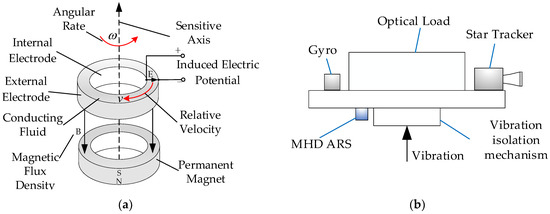
Figure 1.
(a) Schematic diagram of MHD ARS structure; (b) installation principle of MHD ARS.
The vibration of a spacecraft platform reaches the optical load through mechanical transmission. According to the working principle of MHD ARS, it should be fixed on the vertical plane of the vibration axis and ensure that the sensitive axis of MHD ARS is parallel to the vibration axis. Figure 1b shows the installation method of MHD ARS on an optical load. The MHD ARS is installed on the back side of the optical load to ensure that the vibration axis is parallel to the sensitive axis of the MHD ARS. The sensitive axis should be as close to the vibration axis as possible to ensure that the MHD ARS vibrates synchronously with the vibration axis.
3. Improved Algorithm
ACF describes the degree of correlation between the values of a random signal taken at any two different moments. The value of ACF of vibration signal decays slowly with increasing time interval, while the value of ACF of noise signal decays rapidly to zero with increasing time interval [24]. The root mean square (RMS) describes the valid value of a physical quantity, which we use to describe the degree of autocorrelation of the signal at different time intervals. A signal with high dispersion is an effective signal. ACF can be used to distinguish between vibration signal and noise.
Figure 2 shows the overall flow of the algorithm. and are parameters that can be adjusted. is the RMS of the ACF for each IMF, and is the RMS of the ACF for each wavelet coefficient sequence. and are used to determine relevant modes. and are used to improve the threshold. An improved wavelet thresholding function is proposed.
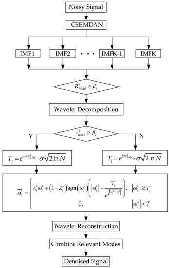
Figure 2.
Flowchart of the improved algorithm.
3.1. Determining Relevant Modes Based on Autocorrelation
CEEMDAN obtains each mode by adding white noise and calculating residual at each decomposition stage. Given a discrete signal , the steps of CEEMDAN can be summarized as follows [25]:
Step1: Add white Gaussian noise to the original signal as follows:
where is the noise factor and is the white noise obeying distribution. , is the times of adding noise.
Step2: Decompose each by EMD. In EMD, the local minimum and maximum of each are calculated by the cubic spline method. The new mode is the average of the minimum and maximum values [26]. The first mode of CEEMDAN is obtained by averaging the new modes. The first residual is obtained by subtracting this first mode calculated from the previous signal.
where IMF1 is the first mode, and is the first residual.
Step3: Repeat all the above steps for the residual and terminate the algorithm when there are no more than two local minimums or maximums in the residual. IMFs and a residual can be obtained as follows:
where is the number of the modes, and is the residual.
The ACF of a discrete series is calculated as follows [24]:
where is the ACF for at time interval , is the length of .
The effective signal is autocorrelated, and its ACF value does not decay rapidly with increasing time intervals. Therefore, its ACF value is highly discrete with respect to the mean value, which means that the RMS value is larger. The RMS of the ACF for each mode is calculated as follows:
is the set threshold. According to the principle of ACF, when choosing the value of , the amplitude range of the effective signal should be taken into account, as should the possibility of mode mixing [25], a phenomenon in which the effective signal is decomposed into multiple modes, resulting in small values for some of the relevant modes. When , the IMF is a relevant mode.
3.2. Improved Wavelet Threshold Based on Autocorrelation
Wavelet transform decomposes the original signal into detail coefficients (cD) and approximate coefficients (cA) [27]. The wavelet decomposition process is shown in Figure 3. In the process, the wavelet coefficients of the signal tend to be stable with the increase in the number of decomposition layers, and the wavelet coefficients of the noise gradually decrease [28].
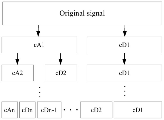
Figure 3.
Wavelet decomposition.
Wavelet transform is a linear transformation [29]. The wavelet coefficients of the signal have obvious autocorrelation, while the wavelet coefficients of the noise have weak or no autocorrelation. The autocorrelation of the wavelet coefficients is used to adjust the threshold.
is the ACF of wavelet coefficients for each frequency band. The RMS of the ACF for wavelet coefficients in different frequency bands is calculated as follows:
where is the number of wavelet coefficients, is the number of the frequency bands.
The Universal Threshold was proposed by Donoho and Johnstone [30]. The Universal Threshold is given as follows:
where is the noise standard deviation, is the data length.
The standard deviation of the noise is calculated as follows [31]:
where is the median of all detail coefficients at each scale [32].
We improved the Universal Threshold by exploiting the ACF of the wavelet coefficients. The improved threshold is given as follows:
where represents the wavelet threshold of different frequency bands. is the set threshold. According to the principle of ACF, when choosing the value of , these cases should be considered: the amplitude range of the effective signal; mode mixing causes small values of the relevant modes; and the absolute value of the wavelet coefficients of the decomposed effective signal being larger than that of the noise. and can adjust the exponent to prevent it from being too large or too small, which would increase the computational effort.
When , it indicates that there is an effective signal in this frequency band. and are monotonically decreasing, monotonically increasing exponential functions, respectively. The value of decreases rapidly as increases, and the value of increases rapidly as decreases. The above-mentioned properties can be used to change the threshold size adaptively in each frequency band. When the autocorrelation of the signal meets the requirement, is used to adjust the threshold becomes smaller, so that some weak signals can be retained. Otherwise, is used to adjust the threshold to become larger and remove more noise.
3.3. Improved Thresholding Function
Conventional wavelet thresholding functions have obvious shortcomings. The hard thresholding function is discontinuous at the threshold, and the reconstructed signal will generate additional oscillation. The soft thresholding function compresses the wavelet coefficients larger than the threshold, which can easily cause signal distortion. Both of these conventional thresholds lack adaptability [33]. The following hard and soft thresholding function formulas are given as [34].
In order to overcome the shortcomings of conventional wavelet soft and hard thresholding, we improved the thresholding function as follows:
where, represents the wavelet coefficient sequences of different frequency bands, represents the adjusted wavelet coefficients. is a scale factor, which can adjust the change trend of the thresholding function between soft and hard thresholds. is an adjustment parameter, .
3.3.1. Continuity Analysis
ensures that the improved thresholding function is continuous at . Therefore, the proposed thresholding function can overcome the disadvantages of the hard thresholding function.
3.3.2. Deviation Analysis
When , , the improved thresholding function is a hard thresholding function. When , , the deviation of the improved thresholding function from the hard thresholding function is shown as follows:
ensures that the deviation of the improved thresholding function from the hard thresholding function is zero at infinity.
By choosing the appropriate , the improved thresholding function can be made to converge quickly to the hard thresholding function. This reduces the reconstruction error caused by compressing wavelet coefficients. makes the algorithm more flexible and can be applied to different working environments.
Figure 4 shows the denoising characteristics of the proposed thresholding function and the conventional thresholding functions. It can be observed that the improved thresholding function approximates the hard thresholding function more and more rapidly as decreases. The improved thresholding function overcomes the shortcomings of the conventional thresholding functions. Since the improved thresholding function is continuous at and does not produce additional oscillation like the hard thresholding function, it can enhance the smoothness of the denoised signal and effectively protect the details of the signal. Since it does not compress the wavelet coefficient sequence larger than the threshold as the soft thresholding function, it does not cause signal distortion after reconstruction.
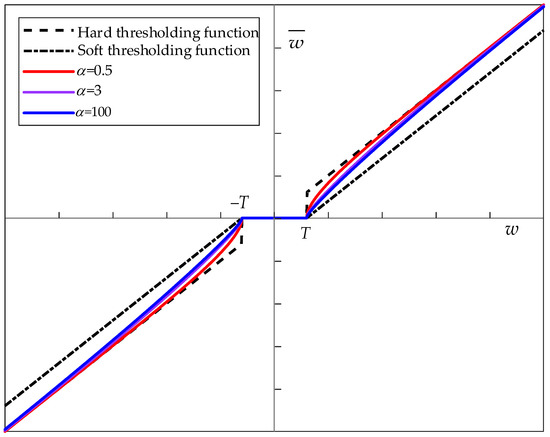
Figure 4.
Image of the proposed thresholding function.
4. Experimental Platform and Result Analysis
In this experiment, we acquired the signals of the MHD ARS measurement system in static and dynamic conditions. The experimental platform is shown in Figure 5. The two-axis turntable generates angular vibration on the azimuth axis. The pitch plane is perpendicular to the azimuth axis. Power supply for motors and MAD ARS. AD conversion module and computer for data acquisition and storage. The resolution of the AD module is 0.9 mV. The algorithms are performed using the computer. We fixed the MHD ARS on the pitch plane of the two-axis turntable and placed it as close as possible to the center point of the pitch plane.
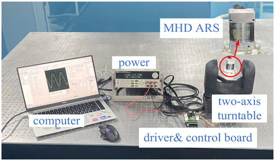
Figure 5.
MHD ARS measurement system experimental platform.
4.1. Static Test Analysis
In this test, after energizing the MHD ARS for 30 min, static data were recorded with a sampling frequency of 100 Hz for 1 h. In CEEMDAN, we set the noise factor of the added gaussian white noise to 0.1. To ensure the denoising effect and save on computational costs, we set the times of adding noise to 100 and the maximum number of iterations to 300. Considering the output of the MHD ARS in the experiment is in the millivolt range and the mode mixing, and were both chosen as 0.0005. The mother wavelet function was sym6, and the decomposition scale was 5 layers. We set to 1000 and to 0.001. To remove as much noise as possible, was 0.1. The IMFs are shown in Figure 6.
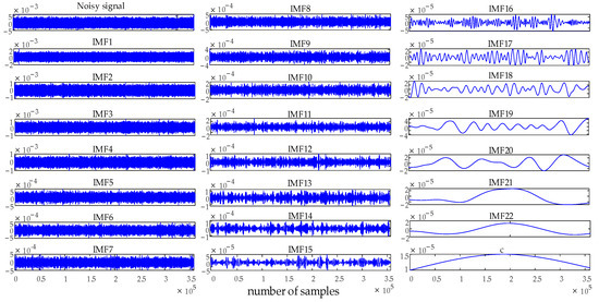
Figure 6.
IMFs of MHD ARS signal in static condition.
Considering that conventional CEEMDAN-WTD have been applied to signal denoising [20,21,22,23], we used the CEEMDAN, CEEMDAN-hard thresholding, and CEEMDAN-soft thresholding algorithms to compare the effects of the improved method. Figure 7 shows the of the IMFs. Figure 8 shows the effects of several methods for denoising, the proposed method significantly reduces the base drift.
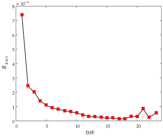
Figure 7.
of the IMFs.
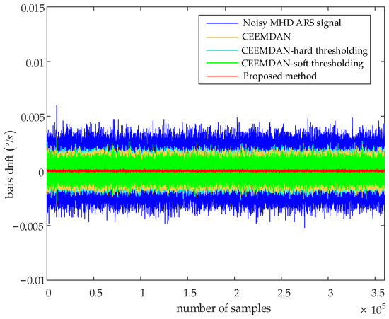
Figure 8.
Denoising results of MHD ARS signal in static condition.
The Allan variance can be quantified and analyzed as, for example, the quantization noise (Q), angle random walk (N), bias instability (B), rate random walk (K), rate ramp (R) and other noise sources [35]. We performed the Allan variance analysis on the MHD ARS denoised signal under the static condition. As shown in Figure 9, in the curve of the noise signal, the slope of the oblique part is close to −1/2, and the slope of the straight part is close to zero. Is indicates that the main noise of the measurement system is the angle random walk and bias instability. The proposed method has the lowest curve.
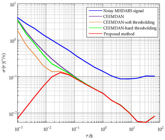
Figure 9.
Allan variance analysis of MHD ARS signal in static condition.
The Allan variance results for random noise are listed in Table 1. As can be seen, the quantization noise is reduced by 10 times as compared to the noisy signal, the angle random walk is reduced by 30 times, and the bias instability is reduced by 1.75 times. The method proposed in this paper has advantages over conventional methods in the static test.

Table 1.
Allan variance analysis results of MHD ARS signal in static condition.
4.2. Dynamic Test Analysis
The working bandwidth of the MHD ARS is 2–1000 Hz. We used the azimuth motor of the turntable to generate angular vibrations of different frequencies to simulate the harmonic vibrations of a spacecraft. In order to verify the effectiveness of the proposed method under the dynamic condition, several single-frequency signals were tested. We acquired the angular vibration signals with different frequencies of 5 Hz, 10 Hz, and 15 Hz with a sampling frequency of 2 kHz and filtered the noisy MHD ARS signals.
The angular vibration can be expressed as follows:
where is the amplitude of the angular vibration and is the frequency. The angular rate of the angular vibration can be expressed as follows:
In this test, the amplitude of the angular vibration is at the microradian level, and the output of the MHD ARS is at the millivolt level. In CEEMDAN, mode mixing results in relatively small magnitudes for the relevant modes. For the above reasons, the parameters were the same as the settings of the static experiment. We used the angular rate measured by an optical encoder system mounted on the azimuth axis as the true angular rate. We acquired single-frequency angular vibration signals at 5 Hz, 10 Hz, and 15 Hz with different angular rates.
As shown in Figure 10, the vibration signals at each frequency contain three amplitudes. At 5 Hz, the angular rates of the vibrations are 0.300°/s, 0.200°/s, and 0.100°/s. At 10 Hz, the angular rates of the vibrations are 0.150°/s, 0.100°/s, and 0.050°/s. At 15 Hz, the angular rates of the vibrations are 0.100°/s, 0.050°/s, and 0.025°/s. Figure 11 shows the IMFs and frequency spectrum of the 0.100°/s signal at 15 Hz.
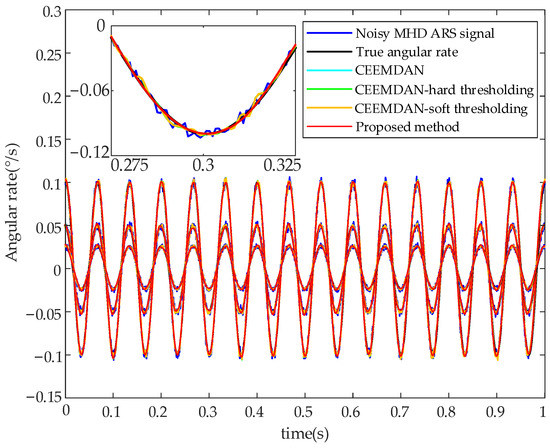
Figure 10.
Denoising results of MHD ARS signals at 15 Hz.
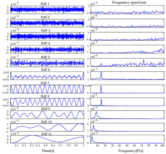
Figure 11.
IMFs and frequency spectrum of the 0.100°/s signal at 15 Hz.
It is observed that the denoised signal obtained by the proposed method is much smoother. Figure 11 shows the IMFs of the 0.100°/s signal at 15 Hz. Figure 12 shows the of the relevant modes. As shown in Figure 11, mode mixing appears in the relevant modes, which results in a larger magnitude of IM7 than the other relevant modes. It is due to the fact that noise affects the selection of the local minimum and maximum values, the average values are obtained from the combination of the noise and the real signal [24]. Noise in the relevant modes IMF5 and IMF6 can be observed.
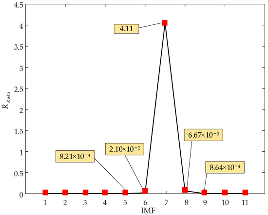
Figure 12.
of the IMFs of the 0.100°/s signal at 15 Hz.
It can be seen from the frequency spectrum in Figure 11 that IMF10 and IMF11 are ineffective modes in low-frequency without the 15 Hz signal, and IMF1-IMF4 are noise modes in high-frequency.
RMSE and SNR are commonly used indicators to evaluate the effect of signal denoising [36].
where is the true vibration signal of the turntable, is the denoised signal. is the signal power, and is the noise power.
In Table 2, Table 3 and Table 4, the RMSE and SNR of vibrations of different angular rates at three frequencies are shown. The RMSE is reduced by 46.58%, and the SNR is improved by 32.75% for the 0.025°/s signal at 15 Hz. The proposed method has the lowest RMSE and the highest percentage of SNR gain for different rates of angular vibration signals at each frequency. It is observed that as the rate decreases, the percentage of SNR gain increases in the improved algorithm. This is because as the rate decreases, the effect of noise on the relevant modes increases. The improved threshold and thresholding function can be used to better advantage.
Table 2.
RMSE and SNR results of MHD ARS signals at 5 Hz.
Table 3.
RMSE and SNR results of MHD ARS signals at 10 Hz.
Table 4.
RMSE and SNR results of MHD ARS signals at 15 Hz.
The harmonic vibration of a spacecraft has high-frequency with low amplitude and low-frequency with high amplitude characteristics [37,38]. To further verify the effectiveness of the proposed method in denoising the MHD ARS dynamic signal, we acquired mixed-frequency angular vibration signals with different amplitudes at 5 Hz, 10 Hz, and 15 Hz.
As shown in Figure 13, the mixed-frequency signal with high amplitude consists of the high amplitude of each frequency. At 5 Hz, the amplitudes of the angular vibrations are 100 , 75 , and 50 , the corresponding angular rates are 0.180°/s, 0.135°/s, and 0.090°/s. At 10 Hz, the amplitudes of the angular vibrations are 25 , 20 , and 15 , the corresponding angular rates are 0.090°/s, 0.072°/s, and 0.054°/s. At 15 Hz, the amplitudes of the angular vibrations are 10 , 8.5 , and 5 , the corresponding angular rates are 0.054°/s, 0.046°/s, and 0.027°/s.
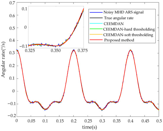
Figure 13.
Denoising results of MHD ARS mixed-frequency signal with high amplitude.
The proposed method has a smoother denoising effect on the mixed-frequency signal with a high amplitude, as shown in Figure 13. Figure 14 and Figure 15 show the IMFs of the mixed-frequency signal with a high amplitude and the of the relevant modes. The signal is decomposed into multiple modes. Mode mixing occurs in the relevant modes, as shown in Figure 14, which results in a larger magnitude of IM8 than the other relevant modes. Noise in the relevant mode IMF6 can be observed.
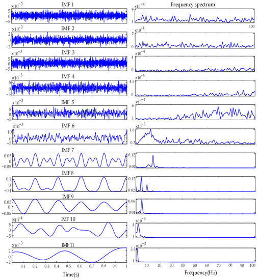
Figure 14.
IMFs and frequency spectrum of MHD ARS the mixed-frequency signal with high amplitude.
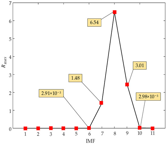
Figure 15.
of MHD ARS mixed-frequency signal with high amplitude.
It can be seen from the frequency spectrum in Figure 13 that IMF11 is an ineffective mode in low-frequency without the mixed-frequency signal, and IMF1-IMF5 are noise modes in high-frequency.
In Table 5, the RMSE and SNR of the MHD ARS mixed-frequency signals with different amplitudes are shown. The RMSE is reduced by 41.65% and the SNR is improved by 16.48% for mixed-frequency signals with a high amplitude. It is observed that the proposed method has the lowest RMSE and the highest percentage of SNR gain for different amplitudes of mixed-frequency angular vibration signals. As with single-frequency signals, the percentage of SNR gain increases as the amplitude decreases in the improved algorithm.
Table 5.
RMSE and SNR results of MHD ARS mixed-frequency signals.
From the dynamic experimental results, it can be seen that the proposed method can effectively improve the SNR and the results are smoother for both single-frequency and mixed-frequency signals.
5. Conclusions
In this paper, an autocorrelation-based CEEMDAN-WTD algorithm is proposed to denoise the static and dynamic signals of the MHD ARS. Firstly, CEEMDAN was used to decompose noisy signal and obtain IMFs, and the autocorrelation of each mode was used to determine the relevant modes. Compared with conventional CEEMDAN, this step could remove ineffective modes in low-frequency and noise IMFs in high-frequency. Then, the autocorrelation of each wavelet coefficient sequence was used to adjust the wavelet threshold. Compared with conventional WTD, this step could remove more noise and retain weak signals. Meanwhile an improved thresholding function was proposed to overcome additional oscillation and reconstruction error in the conventional WTD. Finally, the denoised signal was obtained by combining the denoised relevant modes. Compared with the conventional method, the proposed method could achieve a better denoising effect.
In the static test, the proposed method outperformed the conventional methods. The quantization noise, angle random walk, and bias instability were effectively reduced. In dynamic test, the proposed method improved the SNR and reduced the RMSE more than conventional methods. The denoised signal produced by the proposed method was smoother. As the rate decreased, the effect of noise on the relevant modes increased, the improved threshold and thresholding function achieved a better denoising effect. The tests verified the effectiveness of the proposed method for denoising the angular vibration signal measured by MHD ARS. The proposed method has good prospects in laser communication, gravitational wave detection, and others. Future work is needed to verify the denoising of the angle vibration signals in the three axes and implement it in hardware.
Author Contributions
Conceptualization, Y.S.; methodology, Y.S., C.M. and J.H.; validation, Y.S.; data curation, Y.S., X.W., Y.W. and Z.J. All authors have read and agreed to the published version of the manuscript.
Funding
This work was supported in part by National Key R&D Program of China, Gravitational Wave Detection Project No. 2022YFC2203800.
Institutional Review Board Statement
Not applicable.
Informed Consent Statement
Not applicable.
Data Availability Statement
Not applicable.
Conflicts of Interest
The authors declare no conflict of interest.
References
- Roumelas, G.D.; Nistazakis, H.E.; Leitgeb, E.; Stassinakis, A.N.; Tombras, G.S. On the performance of optical wireless communication links impaired by time jitter, M-turbulence and pointing errors. Opt. Commun. 2020, 472, 126033. [Google Scholar] [CrossRef]
- Danzmann, K.; Rüdiger, A. LISA technology—Concept, status, prospects. Class. Quantum Gravity 2003, 20, S1–S9. [Google Scholar] [CrossRef]
- Wang, X.; Su, X.Q.; Liu, G.Z.; Hang, J.F.; Wang, R. Investigation of high-precision algorithm for the spot position detection for four-quadrant detector. Optik 2020, 203, 163941. [Google Scholar]
- Jennrich, O. LISA technology and instrumentation. Class. Quantum Gravity 2009, 26, 15. [Google Scholar] [CrossRef]
- Xue, Y.Z.; Bo, Q.; Ge, R. Vibration-induced jitter control in satellite optical communication. In Proceedings of the International Symposium on Photoelectronic Detection and Imaging 2013: Laser Communication Technologies and Systems, Beijing, China, 21 August 2013. [Google Scholar]
- Skormin, V.A.; Tascillo, M.A.; Busch, T.E. Demonstration of a Jitter Rejection Technique for Free-Space Laser Communication. IEEE Trans. Aerosp. Electron. Syst. 1994, 2123, 568–576. [Google Scholar]
- Glaese, R.M.; Anderson, E.H.; Janzen, P.C. Active Suppression of Acoustically Induced Jitter for the Airborne Laser. In Proceedings of the Laser Weapons Technology, Orlando, FL, USA, 21 July 2000. [Google Scholar]
- Scozzafava, J.J.; Boroson, D.M.; Burnside, J.W.; Glynn, M.L.; DeVoe, C.E.; DeFranzo, C.M.; Doyle, K.B. Design of a very small inertially stabilized optical space terminal. In Proceedings of the Free-Space Laser Communications VII, San Diego, CA, USA, 27 September 2007. [Google Scholar]
- Ji, Y.; Li, X.F.; Wu, T.F.; Chen, C. Theoretical and experimental study of radial velocity generation for extending bandwidth of magnetohydrodynamic angular rate sensor at low frequency. Sensors 2015, 15, 31606–31619. [Google Scholar] [CrossRef]
- Anspach, J.E.; Sydney, P.F.; Hendry, G. Effects of Base Motion on Space-Based Precision Laser Tracking in the Relay Mirror Experiment. In Proceedings of the International Society for Optics and Photonics, Orlando, FL, USA, 1 August 1991. [Google Scholar]
- Iwata, T.; Hoshino, H.; Yoshizawa, T.; Kawahara, T. Precision attitude determination for the advanced land observing satellite (ALOS): Design, verification, and on-orbit calibration. In Proceedings of the AIAA Guidance, Navigation and Control Conference and Exhibit, Hilton Head, SC, USA, 20 August 2007. [Google Scholar]
- Boroson, D.M.; Biswas, A.; Edwards, B.L. MLCD: Overview of NASA’s Mars laser communications demonstration system. In Proceedings of the Free-Space Laser Communication Technologies XVI, San Jose, CA, USA, 16 June 2004. [Google Scholar]
- Pinney, C.; Hawes, M.A.; Blackburn, J. A cost-effective inertial motion sensor for short-duration autonomous navigation. In Proceedings of the 2003 IEEE International Conference on Intelligent Transportation Systems, Las Vegas, NV, USA, 11–15 April 1994. [Google Scholar]
- Iwata, T.; Kawahara, T.; Muranaka, N.; Laughlin, D.R. High-bandwidth attitude determination using jitter measurements and optimal filtering. In Proceedings of the AIAA Guidance, Navigation, and Control Conference, Chicago, IL, USA, 10–13 August 2009. [Google Scholar]
- Ji, Y.; Du, Y.; Yan, G.; Li, X.; Wu, J.; Tuo, W.; Li, J. Adaptive Kalman filter enhanced with spectrum analysis for wide-bandwidth angular velocity estimation fusion. IEEE Sens. J. 2020, 20, 11527–11536. [Google Scholar] [CrossRef]
- Huang, N.E.; Shen, Z.; Long, S.R.; Wu, M.C.; Shih, H.H.; Zheng, Q.; Yen, N.C.; Tung, C.C.; Liu, H.H. The empirical mode decomposition and the Hilbert spectrum for nonlinear and non-stationary time series analysis. Proc. R. Soc. Lond. Ser. A Math. Phys. Eng. Sci. 1998, 454, 903–995. [Google Scholar] [CrossRef]
- Huang, N.E.; Wu, M.L.; Qu, W.D.; Long, S.R.; Shen, S.S.P. Applications of Hilbert–Huang transform to non-stationary financial time series analysis. Appl. Stoch. Models Bus. Ind. 2003, 19, 245–268. [Google Scholar] [CrossRef]
- Gan, Y.; Sui, L.; Wu, J.; Wang, B.; Zhang, Q.; Xiao, G. An EMD threshold denoising method for inertial sensors. Measurement 2014, 49, 34–41. [Google Scholar] [CrossRef]
- Shen, C.; Li, J.; Zhang, X.; Shi, Y.; Tang, J.; Cao, H.; Liu, J. A noise reduction method for dual-mass micro-electro mechanical gyroscopes based on sample entropy empirical mode decomposition and time-frequency peak filtering. Sensors 2016, 16, 796. [Google Scholar] [CrossRef]
- Abdelkader, R.; Kaddour, A.; Bendiabdellah, A.; Derouiche, Z. Rolling bearing fault diagnosis based on an improved denoising method using the complete ensemble empirical mode decomposition and the optimized thresholding operation. IEEE Sens. J. 2018, 18, 7166–7172. [Google Scholar] [CrossRef]
- Omitaomu, O.A.; Protopopescu, V.A.; Ganguly, A.R. Empirical mode decomposition technique with conditional mutual information for denoising operational sensor data. IEEE Sens. J. 2011, 11, 2565–2575. [Google Scholar] [CrossRef]
- Tian, Z.W.; Jia, Y.F. A method for portable PPG signal dynamic acquisition and denoise based on CEEMDAN and wavelet transform. J. Instrum. 2023, 18, 01023. [Google Scholar] [CrossRef]
- Fang, J.W.; Ren, L.Y.; Tian, J.Y.; Li, G.S. CEEMDAN-Wavelet Threshold Denoising Method on sEMG. In Proceedings of the 2022 11th International Conference on Bioinformatics and Biomedical Science, Nanning, China, 28–30 October 2022. [Google Scholar]
- Onyejekwe, S.; Kang, X.; Ge, L. Evaluation of the scale of fluctuation of geotechnical parameters by autocorrelation function and semi-variogram function. Eng. Geol. 2016, 214, 43–49. [Google Scholar] [CrossRef]
- Torres, M.E.; Colominas, M.A.; Schlotthauer, G.; Flandrin, P. A complete ensemble empirical mode decomposition with adaptive noise. In Proceedings of the 2011 IEEE International Conference on Acoustics, Speech and Signal Processing, Prague, Czech Republic, 22–27 May 2011. [Google Scholar]
- Seyrek, P.; Şener, B.; Özbayoğlu, A.M.; Ünver, H.Ö. An evaluation study of EMD, EEMD, and VMD for chatter detection in milling. Procedia Comput. Sci. 2022, 200, 160–174. [Google Scholar] [CrossRef]
- Mallat, S.G. A theory for multiresolution signal decomposition: The wavelet representation. IEEE Trans. Pattern Anal. Mach. Intell. 1989, 11, 674–693. [Google Scholar] [CrossRef]
- Jiang, J.; Guo, J.; Fan, W.H.; Chen, Q.W. An improved adaptive wavelet denoising method based on neighboring coefficients. In Proceedings of the 2010 8th World Congress on Intelligent Control and Automation, Jinan, China, 7–9 July 2010. [Google Scholar]
- Cai, Y.; Yu, C.M.; Ren, Y.; Wang, W.J.; Yin, Z.Y.; Xia, C.F. High precision attitude-rate measurement of magnetically suspended control and sensing gyroscope using variational mode decomposition and wavelet transform. IEEE Sens. J. 2022, 22, 1188–1198. [Google Scholar] [CrossRef]
- Donoho, D. De-noising by soft-thresholding. IEEE Trans. Inf. Theory 1995, 41, 613–627. [Google Scholar] [CrossRef]
- Jang, Y.I.; Sim, J.Y.; Yang, J.R.; Kwon, N.K. The optimal selection of mother wavelet function and decomposition level for denoising of DCG signal. Sensors 2021, 21, 1851. [Google Scholar] [CrossRef]
- Shi, Y.B.; Zhang, J.J.; Jiao, J.J.; Zhao, R.; Cao, H.L. Calibration analysis of high-G MEMS accelerometer sensor based on wavelet and wavelet packet denoising. Sensors 2021, 21, 1231. [Google Scholar] [CrossRef] [PubMed]
- Xu, X.W.; Liang, Y.; He, P.; Yang, J.L. Adaptive motion artifact reduction based on empirical wavelet transform and wavelet thresholding for the non-contact ECG monitoring systems. Sensors 2019, 19, 2916. [Google Scholar] [CrossRef] [PubMed]
- Cao, H.L.; Zhang, Z.; Zheng, Y.; Guo, H.; Zhao, R.; Shi, Y.; Chou, X. A new joint denoising algorithm for high-G calibration of MEMS accelerometer based on VMD-PE-wavelet threshold. Shock Vib. 2021, 2021, 1–16. [Google Scholar] [CrossRef]
- Yang, G.L.; Liu, Y.Y.; Li, M.; Song, S.G. AMA-and RWE-based adaptive Kalman filter for denoising fiber optic gyroscope drift signal. Sensors 2015, 15, 26940–26960. [Google Scholar] [CrossRef] [PubMed]
- Narasimhappa, M.; Sabat, S.L.; Nayak, J. Adaptive sampling strong tracking scaled unscented Kalman filter for denoising the fiber optic gyroscope drift signal. IET Sci. Meas. Technol. 2015, 9, 241–249. [Google Scholar] [CrossRef]
- Wittig, M.E.; Holtz, L.V.; Tunbridge, D.E.L.; Vermeulen, H.C. In-Orbit Measurements of Microaccelerations of ESA’s Communication Satellite OLYMPUS. In Proceedings of the Free-Space Laser Communication Technologies, Los Angeles, CA, USA, 1 July 1990. [Google Scholar]
- Sudey, J.J.; Schulman, J.R. In-orbit measurements of Landsat-4 thematic mapper dynamic disturbances. Acta Astronaut. 1985, 12, 485–503. [Google Scholar] [CrossRef]


Disclaimer/Publisher’s Note: The statements, opinions and data contained in all publications are solely those of the individual author(s) and contributor(s) and not of MDPI and/or the editor(s). MDPI and/or the editor(s) disclaim responsibility for any injury to people or property resulting from any ideas, methods, instructions or products referred to in the content. |
© 2023 by the authors. Licensee MDPI, Basel, Switzerland. This article is an open access article distributed under the terms and conditions of the Creative Commons Attribution (CC BY) license (https://creativecommons.org/licenses/by/4.0/).