A Fault Section Location Method for Distribution Networks Based on Divide-and-Conquer

Abstract

In this paper, a fault location method based on divide-and-conquer (DAC) is proposed to solve the inadequacy problem that arises when using the traditional fault section location method based on the optimization model of logic operation. The problem is that it is difficult to balance speed and accuracy after the scale of the distribution network is expanded. First, the causal link between fault information and the faulty device was described using the road vector, the equivalent transformation of the logical operations in the traditional model was implemented with the properties of the road vector, and the numerical computational model of the fault location was constructed. Based on this, the optimization-seeking variable “approximation gain” was introduced to prove that the proposed model conforms to the recursive structure of DAC, and the method of applying DAC to locate faults is proposed. The method applies the “Divide-Conquer-Combine” recursive mode to locate faults, and each level of recursion contains only linear-time “approximation gain” operations and constant-time decomposition and combination operations. The efficiency analysis and simulation results show that the proposed method has linear-time complexity and can accurately locate faults in milliseconds, providing a reference for solving the fault location problem in large distribution networks.

1. Introduction

Distribution network fault location is important in improving power system supply reliability as a prerequisite for fault isolation and power supply restoration [1,2]. Modern power distribution systems mostly adopt multi-sectioned and multi-linked network structures so that faults can be limited to a smaller area to meet the increasingly demanding power supply service needs of electricity consumers [3]. However, the increase in the number of sections reduces the supply radius, resulting in insignificant differences in the magnitude of short-circuit currents in adjacent lines, which makes the fault location method based on the traditional three-stage current protection principle no longer applicable [4]. In the meantime, the problems of network scaling, distortion of fault information, and multiple faults in extreme cases also put higher requirements and challenges on the accuracy and speed of fault location [5].

Along with the construction of distribution automation and the development of communication technology, feeder terminal units (FTUs) and other intelligent monitoring devices have become popular [6]. The FTU installed at the intelligent switch can be equipped with fault current detection elements and adaptively adjust the action threshold of the fault current detection elements according to the operation mode of the system [7]. After a fault in the distribution network, the FTU compares the current flowing at the switch with the preset threshold to determine whether a short-circuit current is flowing at the switch, and it reports the fault detection results to the fault location decision host, which applies the fault location algorithm to identify the fault location [8,9]. The basic working principle of the fault location method for distribution networks based on FTU fault information is shown in Figure 1. This method has the advantages of small data communication and convenient implementation, and it has gradually become the main means of fault location in medium-voltage distribution networks [10,11].

Distribution network fault location methods based on FTU fault information mainly include four types: the first type is based on matrix algorithm fault location methods, the second type is based on intelligent optimization algorithm fault location methods, the third type is based on linear integer programming model fault location methods, and the fourth type is fault location methods based on hierarchical optimization models.

(1)

Matrix algorithm-based fault location methods for distribution networks. The basic principle of this method is to construct a fault discrimination matrix based on the topology of the distribution network and the fault information reported by FTUs and locate the faulty equipment via comprehensive analysis of the fault discrimination matrix [12,13]. The matrix algorithm has the advantages of simple principles and fast calculation speed. However, in actual engineering, FTUs are usually installed outdoors and work in harsh environments, resulting in possible misreporting or omission of the reported information. When the fault information is distorted, the matrix constructed by the algorithm cannot correctly reflect the real fault situation, thereby causing the algorithm function to fail [14]. Reference [15] proposes using the adjacency of FTUs measurement points to correct the fault information. Reference [16] proposes introducing telemetry data to check the localization results. However, these methods are only valid for partial cases of fault information distortion [17], and the fault tolerance process of the algorithm additionally increases fault location time. With the expansion of the network scale, the number of FTU measurement points increases, and the probability of fault information distortion increases; thus, the method is difficult to apply to the fault location problem of large distribution networks.

(2)

Fault location methods based on the intelligent optimization algorithm. Reference [18] proposes applying logical operations to express the causal relationship between FTU fault information and faulty equipment and proposes a mathematical model of fault location based on the state approximation principle, which transforms fault location into a combinatorial optimization problem. Since then, scholars have successively used the genetic algorithm (GA) [19], binary particle swarm optimization algorithm (BPSO) [20], ant colony algorithm (AC) [21], harmony search algorithm (HS) [22], and other intelligent algorithms to implement the solution of this model. The intelligent optimization algorithm has a strong information fault tolerance capability. However, the method requires iterative search operations in a high-dimensional solution space, which affects the speed of fault location [23]. Moreover, its search process has a certain degree of randomness, which leads to a certain probability of local convergence. Therefore, this method has the inherent defect of insufficient convergence stability [24].

(3)

Fault location methods based on the linear integer programming model. The basic principle of this method is to transform the mathematical model of fault location into a linear integer programming model (LIP) using algebraic operation substitution [25], ascending dimension [26], etc. Then, classical LIP methods (such as the branch and bound method, cut plane method, and implicit enumeration method) are applied to solve the model to locate the fault. The “optimality checking” step in the LIP solution method enables it to gradually approximate and eventually converge to the global optimal solution through iterations and thus has good convergence stability. However, the solution of the LIP model involves the computation of its continuous relaxed linear programming model (LP) several times, resulting in high time complexity for the algorithm [27]. Tests have shown that the fault location time of small and medium-sized distribution networks is in the range of seconds [26], which does not meet the requirements of rapidity.

(4)

Fault location methods based on the hierarchical optimization model. Reference [28] proposes that the branch of the network is externally equivalent to a two-port based on the equivalence principle and constructs a hierarchical optimization model of fault location. The basic idea is to solve the mathematical model of fault location in a reduced dimension: first, locate the branch where the fault is located, then determine the faulty device from the faulty branch. Since then, scholars have successively used the multiverses optimization algorithm (MVO) [29], quantum computing and immune optimization algorithm(QIOA) [30], bald eagle search algorithm (BES) [31], and other intelligent algorithms to implement the solution of hierarchical optimization models. This method converts effectively reduces the size of solution space and improves the speed and accuracy of fault location. However, the method requires high soundness of FTU fault information at the branch port, which may produce misjudgment when the port information is distorted, and it cannot completely eradicate the defect of insufficient convergence stability of the intelligent algorithm.

The characteristics of the aforementioned various distribution network fault location methods are shown in

Table 1. Characteristics of fault location methods.

Method	Characteristics
Matrix algorithm	It has fast location speed but poor information fault tolerance.
Intelligent optimization algorithm	It has high fault information tolerance, but its computational efficiency and convergence stability are poor.
Linear integer programming algorithm	It has high fault information tolerance and strong convergence stability but poor computational efficiency.
Hierarchical fault location method	Its convergence reliability and computational efficiency are better than the intelligent optimization algorithm, but it requires higher information reliability in port nodes.

.

In summary, a large number of results have been achieved in distribution network fault location methods, but the following problems still exist: on one hand, the traditional fault location model contains logical operations; thus, it is difficult to obtain a high efficient solution to the model through strict mathematical derivation; on the other hand, the current fault location methods are still difficult to use simultaneously. Furthermore, current fault location methods are not yet able to meet the requirements of accuracy and speed simultaneously.

In view of these problems, this paper proposes a fault section location method for a distribution network based on divide-and-conquer (DAC). The following three aspects are the main features of this work:

• The application of road vectors to establish causal links between fault information and faulty equipment, the equivalent transformation of logical operations in the mathematical model of traditional fault location, and the construction of a numerical computational model of fault location.
• Defines “compatible sets” and “approximation gains” and validates its properties, and then proves that the mathematical model constructed in this paper conforms to the recursive structure of DAC.
• Proposes a fault location method based on DAC, which uses the recursive model of “Divide-Conquer-Combine” in each level of recursion. The linear time “approximation gain” computations and constant time divide and combine operations are included in each layer of recursion to improve the computational efficiency while ensuring the accuracy of fault location.

The rest of this paper is organized as follows. In Section 2, the numerical calculation model of fault location is proposed. Section 3 demonstrates the recursive structure of the proposed model. In Section 4, the DAC-based fault location method is proposed, and its computational efficiency is analyzed. In Section 5, the accuracy and computational efficiency of the method in this paper are verified by simulation tests. Section 6 summarizes the paper.

2. Numerical Computational Model for Distribution Grid Fault Location

2.1. Basic Principle of Distribution Network Fault Location

When a fault occurs in the distribution network, the FTU installed at the smart switch (including circuit breakers and section switches) detects the current crossing and uploads the fault detection results to the fault location decision servers, which determines the fault device based on the fault location algorithm. In this paper, we refer to the smart switch equipped with FTU as a node and the distribution line enclosed by the nodes as a section. The task of the fault location is to accurately locate the section where the fault occurs.

With the help of the fault hypothesis theory, the fault location problem can be transformed into a combinatorial optimization problem. The basic principle is as follows: assuming that all possible fault scenarios to construct a solution space, find the optimal solution in the solution space, and this optimal solution can give the most reasonable explanation to the fault information reported by the FTU. This section describes the coding rules of fault information, proposes the corresponding relationship between fault scenarios and fault information, and describes how the combinatorial optimization model for fault location was constructed.

2.1.1. Fault Information Code

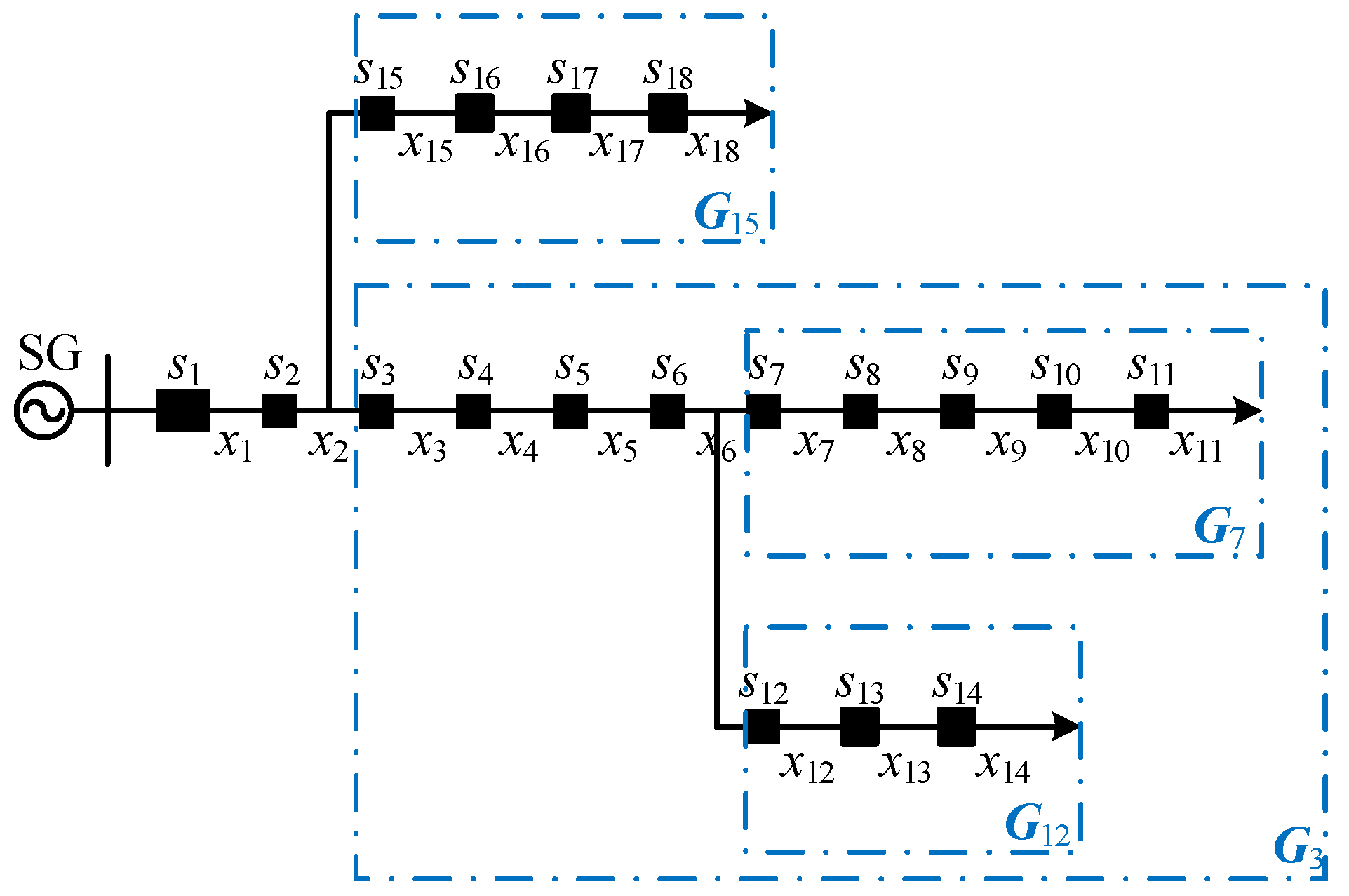
The network structure of a typical distribution network is shown in Figure 2, where SG indicates the main power provided by the substation, and the black squares indicate the nodes. This article specifies that the direction from the main power to the section is the positive direction of the section. For the convenience of the description, the nodes are numbered consecutively according to their distance from the main power, and the section number is taken as the smaller of its associated node number (i.e., the section number is taken as its originating point number). The distribution network shown in Figure 2 is numbered according to these rules, where s₁~s₆ denotes the node number, and x₁~x₆ denotes the section number. In this paper, sections associated with more than two nodes are called T-type sections, e.g., section x₂. In contrast, x₁, x₃~x₆ are called ordinary sections. In addition, in this paper, we applied sets V and E to represent the sets of nodes and sections of the distribution network, respectively, and the distribution network is represented as G = (V, E).

The distribution network has a radial network structure, and when a fault occurs, the fault current flows from the main power to the faulty equipment. For a distribution network containing m nodes, the fault information vector I = [I₁, I₂, …, I_m] indicates the fault information reported by FTUs, where the variables I_i are defined as shown in Equation (1).

$${\mathit{I}}_i=\left\{\begin{array}{l}1\hspace{1em}\mathrm{Node}{s}_i \mathrm{has} \mathrm{flowed}\mathrm{a}\mathrm{short}-\mathrm{circuit}\mathrm{current}\\ 0\hspace{1em}\hspace{1em}\hspace{1em}\hspace{1em}\mathrm{Others}\end{array}\right.$$

(1)

For a distribution network with a number of sections n, apply the variable y_k (k = 1, 2, …, n) to indicate whether section x_k fault, y_k, is defined, as shown in Equation (2).

$$y_k=\left\{\begin{array}{l}1 \mathrm{Section}{x}_k \mathrm{failure}\\ 0 \mathrm{No} \mathrm{failure} \mathrm{in} \mathrm{section} x_k\end{array}\right.$$

(2)

On this basis, our assumed fault scenarios can be described by the set of fault sections X, which is the set consisting of the sections where faults occur, defined as shown in Equation (3).

$$\mathit{X}=\left\{x_k\in \mathit{E}|y_k=1\right\}$$

(3)

2.1.2. Switching Function

To measure the rationality of the fault information interpretation of the assumed fault scenario, it is necessary to construct the corresponding relationship between the set of fault sections X and the fault information. The fault information of node s_i corresponding to X can be represented by the switch function J_i(X). J_i(X) takes X as the independent variable, which means that when the fault scenario of the distribution network is X, the value of the fault information of node s_i is taken when the information reported by node s_i is not misreported or omitted.

The switching function can be constructed based on the causal relationship between nodes and sections. We can take node s₂ in the distribution network shown in Figure 2 as an example. If a fault signal is reported at s₂, it is known that the fault signal at s₂ may be generated by sections x₂~x₆ as caused by the occurrence of a short-circuit fault. Therefore, the operation status of sections x₂~x₆ is related to the fault information of node s₂, and in this paper, sections x₂~x₆ are the causal devices of s₂. Similarly, the causal devices of other nodes in Figure 2 can be determined, as shown in

Table 2. Causal devices corresponding to nodes in the distribution network.

Node	Causal Device (Section)	Status Information of the Causal Device	Total Number
s1	x1~x6	y1~y6	6
s2	x2~x6	y2~y6	5
s3	x3, x4	y3, y4	2
s4	x4	y4	1
s5	x5, x6	y5, y6	2
s6	x6	y6	1

.

Based on this analysis, the logical “OR” operation was introduced to express the causal connection between nodes and sections, and the switching function J_i(X) of node s_i was constructed according to Equation (4):

$${\mathit{J}}_i(\mathit{X})={\displaystyle \prod y_k}$$

(4)

where y_k denotes the causal device of node s_i and “$\prod$” denotes the superposition of logical “OR” operations.

To enhance understanding, the distribution network shown in Figure 2 is taken as an example to illustrate the calculation process of the switching function. Assume the fault scenario X = {x₃, x₆}. The calculation process and results of the switching function of each node are shown in Equation (5).

$$\left\{\begin{array}{l}{\mathit{J}}_1(\mathit{X})=y_1\vee y_2\vee y_3\vee y_4\vee y_5\vee y_6= 0\vee 0\vee 1\vee 0\vee 0\vee 1=1\\ {\mathit{J}}_2(\mathit{X})=y_2\vee y_3\vee y_4\vee y_5\vee y_6=0\vee 1\vee 0\vee 0\vee 1=1\\ {\mathit{J}}_3(\mathit{X})=y_3\vee y_4=1\vee 0=1\\ {\mathit{J}}_4(\mathit{X})=y_4= 0\\ {\mathit{J}}_5(\mathit{X})=y_5\vee y_6= 0\vee 1=1\\ {\mathit{J}}_6(\mathit{X})=y_6= 1\end{array}\right.$$

(5)

where “$\vee$” means the logical “OR” operation.

2.1.3. Objective Function

According to the state approximation theory, the essence of fault location is to find the most likely fault scenario X, where the section state can provide the most reasonable explanation for the fault information reported by FTU. In other words, the smaller the difference between the switching function J_i(X) of the fault sections set X and the fault information I_i actually reported by FTU, i, the more reasonable the interpretation is, and the closer X is to the real fault situation. Therefore, the objective function of fault location is shown in Equation (6) [26]:

$$\min f(\mathit{X})={\displaystyle \sum _{i=1}^m\left[{\mathit{I}}_i\oplus {\mathit{J}}_i(\mathit{X})\right]}+\omega {\displaystyle \sum _{x_k\in \mathit{X}}{y}_k}$$

(6)

where m indicates the total number of nodes in the distribution network, and “$\oplus$“ denotes the logical “XOR” operation. When I_i = J_i(X), ${\mathit{I}}_i\oplus {\mathit{J}}_i(\mathit{X})=0$; otherwise, ${\mathit{I}}_i\oplus {\mathit{J}}_i(\mathit{X})=1$. ω is the error-proof factor, which takes values between 0 and 1.

Take the typical distribution network shown in Figure 1 as an example to illustrate the basic principle of fault location for distribution network. Suppose section x₄ fails, the fault information reported by FTU is I = [I₁~I₆] = [1 1 1 1 1 0 0], and the fault location algorithm is activated. According to Equation (2), each section has two operating states: “normal” and “fault”. As the network contains six sections, there are 2⁶ possible fault scenarios. Each fault scenario can be described by a set of fault sections X, and the 2⁶ X form the solution space, from which the task of fault location is to find the optimal solution. The switch functions and objective functions for some hypothetical fault scenarios are shown in

Table 3. Vector X and its switching function and objective function.

Number	Fault Scenario	X	[J1(X)~J6(X)]	f(X)
1	x1 failure	{x1}	[1 0 0 0 0 0]	3 + ω
2	x2 failure	{x2}	[1 1 0 0 0 0]	2 + ω
3	x3 failure	{x3}	[1 1 1 0 0 0]	1 + ω
4	x4 failure	{x4}	[1 1 1 1 0 0]	ω
5	x5 failure	{x5}	[1 1 0 0 1 0]	3 + ω
6	x6 failure	{x6}	[1 1 0 0 1 1]	4 + ω
7	x1 and x2 failure	{x1, x2}	[1 1 0 0 0 0]	2 + 2ω
8	x1 and x3 failure	{x1, x3}	[1 1 1 0 0 0]	1 + 2ω
…	…	…	…	…
26	x1~x6 failure	{x1, x2, x3, x4, x5, x6}	[1 1 1 1 1 1]	2 + 6ω

.

By comparing the objective functions of 2⁶ assumed failure scenarios, it can be seen that the objective function of number 4 is the smallest; thus, X = {x₄} is taken as the optimal solution. Therefore, section x₄ is determined to be the fault section. The fault location operation is finished, and the result of the fault location is output.

2.2. Construction of the Numerical Computation Model

In this example, we can see that the size of the solution space of the fault location problem is exponentially related to the number of sections in the distribution network. Assuming and comparing all possible fault scenarios to locate the fault section will seriously reduce computational efficiency. Meanwhile, the fault location model contains logical relation operations (such as “OR” operations in Equation (4) and “XOR” operations in Equation (6)), thereby making it impossible to apply the classical optimization algorithm with superior performance in achieving the solution. Although locating faults by means of intelligent algorithms with stochastic search characteristics can improve computational efficiency to a certain extent, they have the inherent defect of insufficient convergence stability, which makes it difficult to guarantee the accuracy of fault location.

In view of these problems, this section proposes to apply the road vector to describe the causal relationship between nodes and sections, to equivalently transform the logical operations in the model by the properties of the road vector, to construct the numerical computation model of fault location, and to lay the theoretical foundation for proposing a faster and more accurate fault location method.

2.2.1. Road Vector

The road that defines the section is the set of nodes and sections on the path from the section to the main power source. For the distribution network containing m nodes, the road vector of section x_k is ${\mathit{P}}_k= [{\mathit{P}}_k\left(1\right), {\mathit{P}}_k\left(2\right), \dots , {\mathit{P}}_k(i),\dots , {\mathit{P}}_k(m\left)\right]$, where the element ${\mathit{P}}_k\left(i\right)$ is defined as follows.

$${\mathit{P}}_k(i)=\left\{\begin{array}{l}1 \mathrm{Node}{s}_i\mathrm{is}\mathrm{on}\mathrm{the}\mathrm{road}\mathrm{of}{x}_k\\ 0\hspace{1em}\hspace{1em}\hspace{1em} \mathrm{Others}\end{array}\right.$$

(7)

Taking the distribution network shown in Figure 2 as an example, nodes s₁~s₄ are on the road of section x₄; thus, the road vector P₄ of x₄ is shown in Equation (8).

$${\mathit{P}}_4=[1 1 1 1 0 0]$$

(8)

Similarly, the road vectors of the other sections in Figure 2 can be determined: ${\mathit{P}}_1=[1 0 0 0 0 0]$, ${\mathit{P}}_2=[1 1 0 0 0 0]$, ${\mathit{P}}_3=[1 1 1 0 0 0]$, ${\mathit{P}}_5=[1 1 0 0 1 0]$, and ${\mathit{P}}_6=[1 1 0 0 1 1]$.

When section x₄ has a fault, nodes s₁~s₄ are on the main power to section x₄ path; thus, nodes s₁~s₄ will flow the fault current and report the fault information. It can be seen that the road vector can describe the causal relationship between nodes and sections. For a hypothetical fault scenario X, the switching function J_i(X) of node i can be rewritten in Equation (4) as

$${\mathit{J}}_i(\mathit{X})={\displaystyle \prod _{x_k\in \mathit{X}}{\mathit{P}}_k\left(i\right)}$$

(9)

Applying the vector J(X) represents the switching function corresponding to the assumed fault scenario X, the vector J(X) = [J₁(X), J₂(X), …, J_m(X)]. The combination of Equation (9) in matrix form and the vector J(X) is shown in Equation (10):

$$\mathit{J}(\mathit{X})={\displaystyle \prod _{x_k\in \mathit{X}}{\mathit{P}}_k}$$

(10)

where “$\prod$” means the superposition operation of “OR” is completed for multiple same-dimension vectors consecutively.

The distribution network shown in Figure 2 is used as an example to verify the effectiveness of the road vector in describing the causal relationship. Assuming the fault scenario X = {x₃, x₆}, according to Equation (10), the vector J(X) is shown in Equation (11):

$$\mathit{J}(\mathit{X})={\displaystyle \prod _{x_k\in \mathit{X}}{\mathit{P}}_k}={\mathit{P}}_3\vee {\mathit{P}}_6=[1 1 1 0 0 0]\vee [1 1 0 0 1 1]=[1 1 1 0 1 1]$$

(11)

where “$\vee$“ means that the corresponding elements of two same-dimension vectors undergo logical “OR” operations.

Equation (11) has the same result as Equation (5), which shows that the road vector can effectively describe the causal relationship between nodes and sections.

2.2.2. Properties of the Road Vector

The properties of the road vector are the basis for constructing and solving numerical computational models of fault location. These properties are stated first, and their mathematical proofs are given in Appendix A.

Theorem 1. 

If the distribution network nodes and sections are numbered using the numbering rules in this paper, the following conclusions are equivalent.

(1)

${\mathit{P}}_j\left(i\right)= 1$;

(2)

Section x_i is on the road of section x_j;

(3)

${\mathit{P}}_i={\mathit{P}}_i\ast {\mathit{P}}_j$;

where “$\ast$” means that the corresponding elements of two same-dimension vectors are multiplied (“$\ast$” satisfies the commutative law and the associative law).

Theorem 2. 

Let the set of sections in the distribution network be $\mathit{E}$. For sections $x_i,x_j,x_r\in \mathit{E}$, at least one of the following expressions holds:

$${\mathit{P}}_i\ast {\mathit{P}}_j\ast \left(\mathit{e}-{\mathit{P}}_r\right)=0$$

(12)

$${\mathit{P}}_i\ast {\mathit{P}}_r\ast \left(\mathit{e}-{\mathit{P}}_j\right)=0$$

(13)

where e denotes a vector of the same dimension as the road vector, and the element values are all 1.

Theorem 3. 

Let the set of sections in the distribution network be $\mathit{E}$, let $\mathit{X}\subseteq \mathit{E}$ be a subset of sections, and suppose section  $x_i\in \mathit{E}-\mathit{X}$. If ${\mathit{P}}_i\ast {\displaystyle \prod _{x_k\in \mathit{X}}^{\ast }\left(\mathit{e}-{\mathit{P}}_k\right)}=0$, then $\exists x_k\in \mathit{X}$ such that ${\mathit{P}}_i={\mathit{P}}_i\ast {\mathit{P}}_k$

Where “${\displaystyle \prod ^{\ast }}$” means that the superposition operation of “$\ast$“ is performed for multiple same-dimension vectors consecutively.

2.2.3. Numerical Computational Expressions for the Switching Function

This section equivalent transforms the logic “OR” operation in Formula (10) of the switching function based on the properties of the road vector and deduces the numerical calculation expression of the switching function.

We claim that the following numerical computational relationship exists between the hypothetical fault scenario X and the switching function vector J(X):

$$\mathit{e}-\mathit{J}(\mathit{X})={\displaystyle \prod _{x_k\in \mathit{X}}^{\ast }\left(\mathit{e}-{\mathit{P}}_k\right)}$$

(14)

The mathematical induction method is applied for the proof. Use the data structure “Queue” to represent X, X = {x_k1, x_k2, …, x_p, x_p+1, …}. Let X_u be the queue consisting of the first u elements of X.

$${\mathit{X}}_u=\{x_{kz}\in \mathit{X}|1\le kz\le u\}$$

(15)

(1)

When u = 1, by Equation (10), $\mathit{J}({\mathit{X}}_1)={\mathit{P}}_{k1}$. Obviously, $\mathit{e}-\mathit{J}({\mathit{X}}_1)=\mathit{e}-{\mathit{P}}_{k1}$.

(2)

Suppose that $\mathit{e}-\mathit{J}({\mathit{X}}_p)={\displaystyle \prod _{x_k\in {\mathit{X}}_p}^{\ast }\left(\mathit{e}-{\mathit{P}}_k\right)}$ when u = p. When u = p + 1, we apply Equation (10) to expand $\mathit{J}({\mathit{X}}_{p+1})$:

$$\mathit{e}-\mathit{J}({\mathit{X}}_{p+1})=\mathit{e}-({\mathit{P}}_{k1}\vee {\mathit{P}}_{k2}\vee \dots \vee {\mathit{P}}_{kp}\vee {\mathit{P}}_{kp+1})=\mathit{e}-\left[\mathit{J}({\mathit{X}}_p)\vee {\mathit{P}}_{kp+1}\right]$$

(16)

Because for any 0–1 vector a, b, we have $\mathit{a}\vee \mathit{b}=\mathit{a}+\mathit{b}-\mathit{a}\ast \mathit{b}$, $\mathit{a}-\mathit{a}\ast \mathit{b}=\mathit{a}\ast (\mathit{e}-\mathit{b})$,

$$\begin{array}{cc}\mathit{e}-\mathit{J}({\mathit{X}}_{p+1})& =\mathit{e}-\left[\mathit{J}({\mathit{X}}_p)+{\mathit{P}}_{kp+1}-\mathit{J}({\mathit{X}}_p)\ast {\mathit{P}}_{kp+1}\right]\\ & =\mathit{e}-\left\{\mathit{J}({\mathit{X}}_p)+\left[\mathit{e}-\mathit{J}({\mathit{X}}_p)\right]\ast {\mathit{P}}_{kp+1}\right\}=\left[\mathit{e}-\mathit{J}({\mathit{X}}_p)\right]\ast \left(\mathit{e}-{\mathit{P}}_{kp+1}\right) \end{array}$$

(17)

Substituting the assumptions $\mathit{e}-\mathit{J}({\mathit{X}}_p)={\displaystyle \prod _{x_k\in {\mathit{X}}_p}^{\ast }\left(\mathit{e}-{\mathit{P}}_k\right)}$ into Equation (17), we obtain

$$\mathit{e}-\mathit{J}({\mathit{X}}_{p+1})=\left(\mathit{e}-{\mathit{P}}_{kp+1}\right)\ast {\displaystyle \prod _{x_k\in {\mathit{X}}_p}^{\ast }\left(\mathit{e}-{\mathit{P}}_k\right)}={\displaystyle \prod _{x_k\in {\mathit{X}}_{p+1}}^{\ast }\left(\mathit{e}-{\mathit{P}}_k\right)}$$

(18)

This proves that Equation (14) holds. By shifting the terms of Equation (14), the numerical expression of the switching function is obtained as follows.

$$\mathit{J}(\mathit{X})=\mathit{e}-{\displaystyle \prod _{x_k\in \mathit{X}}^{\ast }\left(\mathit{e}-{\mathit{P}}_k\right)}$$

(19)

2.2.4. Numerical Computational Expression for the Minimum Fault Set Constraint

In Equation (6) of the objective function calculation for fault location, we introduced a second term to the right side of the equation. This is due to the possibility that the minimum value of the first term of Equation (6) corresponds to multiple assumed fault scenarios. Taking the distribution network shown in Figure 2 as an example, assuming section x₃ faults, the fault information reported by the FTUs is I = [I₁~I₆] = [1 1 1 0 0 0]. For the assumed fault scenarios X₁ = {x₃}, X₂ = {x₁,x₃}, X₃ = {x₂,x₃}, X₄ = {x₁,x₂,x₃}, according to Equation (19) of the switching function, we can obtain J(X₁) =J(X₂) = J(X₃) = J(X₄) = [1 1 1 0 0 0] = I (the same results can be obtained by applying the logical expression (10) of the switching function because the two are equivalent), substituting the first term of Equation (6): ${\displaystyle \sum _{i=1}^n\left[{\mathit{I}}_i\oplus {\mathit{J}}_i(\mathit{X})\right]}= 0$. That is, the assumed fault scenarios X₁~X₄ all lead to the minimum value of the first term of Equation (6).

This phenomenon has been discussed in more depth in [18], and the theory of “minimum fault set” has been proposed to solve this problem. The meaning of the “minimum fault set” theory is that the fault scenario with the lowest number of fault sections has the highest probability of occurrence. The mathematical description is as follows: for the set of fault sections X, if there exists a proper subset X′ of X such that J(X) = J(X′), then X is determined to be an infeasible solution that does not satisfy the “minimum fault set” constraint. Taking this fault case as an example, X₁ is a proper subset of X₂~X₄ with J(X₁) = J(X₂) = J(X₃) = J(X₄); thus, X₂~X₄ is an infeasible solution that does not satisfy the “minimum fault set” constraint; thus, the unique optimal solution X₁ can be determined.

For the application of the “minimum fault set” constraint, it is common to add a penalty function to modify the objective function (e.g., the second term in Equation (6)) to ensure that the result of the fault location satisfies the “minimum fault set” requirement. However, this will expand the number of feasible solutions, which is not conducive to improving computational efficiency.

In this paper, we propose applying the numerical computational expression of the road vector to express the “minimum fault set” constraint. Considering that in these fault scenarios, sections x₁ and x₂ are on the road of x₃, the following inference was made according to Theorem 1.

The set of fault sections X satisfying the minimum fault set constraint is equivalent to the following numerical computational expression.

$$\forall x_i,x_j\in \mathit{X},{\mathit{P}}_i\ne {\mathit{P}}_i\ast {\mathit{P}}_j$$

(20)

The meaning of Equation (20) is that the sections in the set of fault sections X are not on each other’s road, which is a sufficient and necessary condition for X to satisfy the “minimum fault set” constraint. The proof is given below.

(1)

Necessity. Suppose for the sake of contradiction that the set of fault sections $\mathit{X}$ satisfies the “minimum fault set” constraint but $\exists x_i,x_j\in \mathit{X}$ such that ${\mathit{P}}_i={\mathit{P}}_i\ast {\mathit{P}}_j$. Then: ${\mathit{P}}_i-{\mathit{P}}_i\ast {\mathit{P}}_j={\mathit{P}}_i\ast (\mathit{e}-{\mathit{P}}_j)=0$. Let ${\mathit{X}}_a=\mathit{X}-x_i$, ${\mathit{X}}_b={\mathit{X}}_a-x_j$, according to Equation (19):

$$\begin{array}{ll}\mathit{J}(\mathit{X})& =\mathit{e}-{\displaystyle \prod _{x_k\in \mathit{X}}^{\ast }(\mathit{e}-{\mathit{P}}_k)}=\mathit{e}-\left[(\mathit{e}-{\mathit{P}}_i)\ast (\mathit{e}-{\mathit{P}}_j)\right]\ast {\displaystyle \prod _{x_k\in {\mathit{X}}_b}^{\ast }(\mathit{e}-{\mathit{P}}_k)}\\ & =\mathit{e}-\left[\mathit{e}-{\mathit{P}}_i\ast (\mathit{e}-{\mathit{P}}_j)-{\mathit{P}}_j\right]\ast {\displaystyle \prod _{x_k\in {\mathit{X}}_b}^{\ast }(\mathit{e}-{\mathit{P}}_k)}\\ & =\mathit{e}-(\mathit{e}-{\mathit{P}}_j)\ast {\displaystyle \prod _{x_k\in {\mathit{X}}_b}^{\ast }(\mathit{e}-{\mathit{P}}_k)}=\mathit{J}({\mathit{X}}_a)\end{array}$$

(21)

${\mathit{X}}_a$ is a proper subset of $\mathit{X}$, contradicting the assumption that $\mathit{X}$ satisfies the “minimum fault set” constraint.

(2)

Sufficiency. Suppose for the sake of contradiction that $\forall x_i,x_j\in \mathit{X}$, ${\mathit{P}}_i\ne {\mathit{P}}_i\ast {\mathit{P}}_j$, but the set of fault section $\mathit{X}$ does not satisfy the “minimum fault set” constraint. Then, there exists a proper subset ${\mathit{X}}_a$ of $\mathit{X}$ such that $\mathit{J}({\mathit{X}}_a)=\mathit{J}(\mathit{X})$. Let ${\mathit{X}}_b=\mathit{X}-{\mathit{X}}_a$, and ${\mathit{X}}_b\ne \varnothing$. Then: $\mathit{X}={\mathit{X}}_a\cup {\mathit{X}}_b$. According to Equations (14) and (19):

$$\begin{array}{ll}\mathit{J}(\mathit{X})& =\mathit{e}-{\displaystyle \prod _{x_k\in \mathit{X}}^{\ast }(\mathit{e}-{\mathit{P}}_k)}=\mathit{e}-{\displaystyle \prod _{x_k\in {\mathit{X}}_a}^{\ast }(\mathit{e}-{\mathit{P}}_k)}\ast {\displaystyle \prod _{x_k\in {\mathit{X}}_b}^{\ast }(\mathit{e}-{\mathit{P}}_k)}\\ & =\mathit{e}-\left[\mathit{e}-\mathit{J}({\mathit{X}}_a)\right]\ast \left[\mathit{e}-\mathit{J}({\mathit{X}}_b)\right]\\ & =\mathit{J}({\mathit{X}}_a)+\mathit{J}({\mathit{X}}_b)-\mathit{J}({\mathit{X}}_a)\ast \mathit{J}({\mathit{X}}_b)\end{array}$$

(22)

Because $\mathit{J}({\mathit{X}}_a)=\mathit{J}(\mathit{X})$, $\mathit{J}({\mathit{X}}_b)-\mathit{J}({\mathit{X}}_a)\ast \mathit{J}({\mathit{X}}_b)=0$, i.e.,$\mathit{J}({\mathit{X}}_b)\ast \left[\mathit{e}-\mathit{J}({\mathit{X}}_a)\right]=0$. Let $x_i\in {\mathit{X}}_b$ and ${\mathit{X}}_c={\mathit{X}}_b-x_i$. According to Equation (19):

$$\begin{array}{ll}\mathit{J}({\mathit{X}}_b)\ast \left[\mathit{e}-\mathit{J}({\mathit{X}}_a)\right]& =\left[\mathit{e}-{\displaystyle \prod _{x_k\in {\mathit{X}}_b}^{\ast }(\mathit{e}-{\mathit{P}}_k)}\right]\ast \left[\mathit{e}-\mathit{J}({\mathit{X}}_a)\right]\\ & =\left[\mathit{e}-(\mathit{e}-{\mathit{P}}_i)\ast {\displaystyle \prod _{x_k\in {\mathit{X}}_c}^{\ast }(\mathit{e}-{\mathit{P}}_k)}\right]\ast \left[\mathit{e}-\mathit{J}({\mathit{X}}_a)\right]\\ & =\left[\mathit{e}-{\displaystyle \prod _{x_k\in {\mathit{X}}_c}^{\ast }(\mathit{e}-{\mathit{P}}_k)}\right]\ast \left[\mathit{e}-\mathit{J}({\mathit{X}}_a)\right]+{\mathit{P}}_i\ast \left[\mathit{e}-\mathit{J}({\mathit{X}}_a)\right]\ast {\displaystyle \prod _{x_k\in {\mathit{X}}_c}^{\ast }(\mathit{e}-{\mathit{P}}_k)}\\ & =0\end{array}$$

(23)

The two preceding and following terms on the right-hand side of Equation (23) are both 0–1 vectors; thus, they are both 0 vectors by adding them to equal the 0 vector. According to Equation (14), $\left[\mathit{e}-\mathit{J}({\mathit{X}}_a)\right]={\displaystyle \prod _{x_k\in {\mathit{X}}_a}^{\ast }\left(\mathit{e}-{\mathit{P}}_k\right)}$, substitute the latter term on the right-hand side of Equation (23):

$$\begin{array}{ll}{\mathit{P}}_i\ast \left[\mathit{e}-\mathit{J}({\mathit{X}}_a)\right]\ast {\displaystyle \prod _{x_k\in {\mathit{X}}_c}^{\ast }(\mathit{e}-{\mathit{P}}_k)}=& {\mathit{P}}_i\ast {\displaystyle \prod _{x_k\in {\mathit{X}}_a}^{\ast }\left(\mathit{e}-{\mathit{P}}_k\right)}\ast {\displaystyle \prod _{x_k\in {\mathit{X}}_c}^{\ast }(\mathit{e}-{\mathit{P}}_k)}\\ & ={\mathit{P}}_i\ast {\displaystyle \prod _{x_k\in {\mathit{X}}_a\cup {\mathit{X}}_c}^{\ast }(\mathit{e}-{\mathit{P}}_k)}=0\end{array}$$

(24)

According to Theorem 3, $\exists x_j\in {\mathit{X}}_a\cup {\mathit{X}}_c$ such that ${\mathit{P}}_i={\mathit{P}}_i\ast {\mathit{P}}_j$, where $x_i\in {\mathit{X}}_b\subseteq \mathit{X}$, $x_j\in {\mathit{X}}_a\cup {\mathit{X}}_c\subseteq \mathit{X}$, contradicting the assumption that $\forall x_i,x_j\in \mathit{X}$, ${\mathit{P}}_i\ne {\mathit{P}}_i\ast {\mathit{P}}_j$.

This proves that this inference holds.

2.2.5. Numerical Computational Expression for the Objective Function

When considering the minimum fault set constraint, the objective function shown in Equation (6) can be simplified and rewritten in matrix form, as shown in Equation (25):

$$\min f(\mathit{X})={\mathit{e}}^{\mathit{T}}\left[\mathit{I}\oplus \mathit{J}(\mathit{X})\right]$$

(25)

where “$\oplus$ “ means that the corresponding elements of two same-dimension vectors undergo logical “XOR” operations.

The vectors $\mathit{I}$ and $\mathit{J}(\mathit{X})$ are both 0–1 vectors. Because for any 0–1 vector a, b, we have ${\mathit{e}}^{\mathit{T}}\left(a\oplus b\right)={\left(a-b\right)}^{\mathit{T}}\left(a-b\right)$, we can translate Equation (25) into a numerical expression as shown in Equation (26).

$$\min f(\mathit{X})={\left[\mathit{I}-\mathit{J}(\mathit{X})\right]}^{\mathit{T}}\left[\mathit{I}-\mathit{J}(\mathit{X})\right]$$

(26)

In summary, we complete the equivalent transformation of the logical operations in the fault location model by using Equation (26) as the objective function, Equation (19) as the equality constraint, and Equation (20) as the inequality constraint to construct the numerical computational model for fault location, as shown in Equation (27).

$$\left\{\begin{array}{l}\min f(\mathit{X})={\mathit{e}}^{\mathit{T}}\left[\mathit{I}\oplus \mathit{J}(\mathit{X})\right]\\ \mathit{J}(\mathit{X})=\mathit{e}-{\displaystyle \prod _{x_k\in \mathit{X}}^{\ast }\left(\mathit{e}-{\mathit{P}}_k\right)}\\ \forall x_i,x_j\in \mathit{X},{\mathit{P}}_i\ne {\mathit{P}}_i\ast {\mathit{P}}_j\end{array}\right.$$

(27)

It can be seen in Equation (27) that the numerical computation model for fault location does not contain logical operations, which lays a theoretical foundation for a highly efficient solution for the model obtained through strict mathematical derivation.

3. Recursive Structure of Fault Location for the Distribution Network

Divide-and-conquer (DAC) is a classical algorithm design strategy whose core idea is to apply the recursive mode of “divide-conquer-combine” to solve the target problem in a reduced dimension, which is an effective means to improve the efficiency of the algorithm [32]. In this section, we introduce the concepts of “compatibility sets” and “approximation gains” to demonstrate the recursive structure of the fault location problem and provide theoretical support for applying DAC to locate faults in distribution networks quickly and accurately.

3.1. Theoretical Foundation

3.1.1. Compatible Sets

Let $\mathit{E}$ be the set of sections in the distribution network, $\mathit{X}\subseteq \mathit{E}$ be the set of fault sections, and $x_i\in \mathit{X}$. The meaning of the compatible set of section $x_i$ is the condition that the road vector ${\mathit{P}}_k$ of the other sections $x_k\in \mathit{X}-x_i$ in $\mathit{X}$ should be satisfied for $\mathit{X}$ to satisfy the inequality constraint described in Equation (20). We define the compatible set $C_i$ of section $x_i$ according to the inequality constraint expression (20).

$$C_i=\{x_k\in \mathit{E}|{\mathit{P}}_i\ne {\mathit{P}}_i\ast {\mathit{P}}_k \& {\mathit{P}}_k\ne {\mathit{P}}_i\ast {\mathit{P}}_k\}$$

(28)

The properties of compatible sets are the basis of the argument for recursive structures. These properties are stated first, and their mathematical proofs are given in Appendix B.

Theorem 4. 

Let the set of sections in the distribution network be $\mathit{E}$, sets of fault sections be ${\mathit{X}}_a,{\mathit{X}}_b\subseteq \mathit{E}$, and ${\mathit{X}}_a\cup {\mathit{X}}_b=\varnothing$. Then, ${\mathit{X}}_a\cup {\mathit{X}}_b$ satisfies the inequality constraint equivalent to the following conclusion: ${\mathit{X}}_a,{\mathit{X}}_b$ satisfies the inequality constraint and $\forall x_i\in {\mathit{X}}_a$, ${\mathit{X}}_b\subseteq C_i$.

Theorem 5. 

If section $x_i$ is on the road of section $x_k$, then $C_i\subseteq C_k$.

Theorem 6. 

If section $x_i$ is on the road of section $x_k$ and the path from $x_k$ to $x_i$ does not contain a T-type section, then $C_i=C_k$.

3.1.2. Approximation Gains

Let the set of sections in the distribution network be $\mathit{E}$, $\mathit{X}\subseteq \mathit{E}$ be the set of fault sections, and section $x_i\notin \mathit{X}$. The approximation gain of section $x_i$ to $\mathit{X}$ describes the contribution to reducing the objective function $f(\mathit{X})$ after section $x_i$ is added to $\mathit{X}$ (that is, section $x_i$ is determined to be the fault section). The approximate gain of section $x_i$ to set $\mathit{X}$ is shown in Equation (29).

$${\Delta }_i^{\mathit{X}}=f(\mathit{X})-f(\mathit{X}\cup x_i)$$

(29)

By expanding $f(\mathit{X})$ and $f(\mathit{X}\cup x_i)$ with Equation (26) and substituting Equation (19) for $\mathit{J}(\mathit{X})$, the equation for ${\Delta }_i^{\mathit{X}}$ can be deduced:

$${\Delta }_i^{\mathit{X}}={\left[\left(2\mathit{I}-\mathit{e}\right)\ast {\displaystyle \prod _{x_k\in \mathit{X}}^{\ast }\left(\mathit{e}-{\mathit{P}}_k\right)}\right]}^{\mathit{T}}{\mathit{P}}_i$$

(30)

In particular, if $\mathit{X}$ is the empty set, i.e., $\mathit{X}=\varnothing$, then the superscript of ${\Delta }_i^{\varnothing }$ can be omitted and abbreviated as ${\Delta }_i$, which is referred to as the approximation gain of section $x_i$, as shown in Equation (31).

$${\Delta }_i=f(\varnothing )-f(i)$$

(31)

Substitute ${\displaystyle \prod _{x_k\in \varnothing }^{\ast }\left(\mathit{e}-{\mathit{P}}_k\right)}=\mathit{e}$ into Equation (30) to obtain the calculation formula of ${\Delta }_i$.

$${\Delta }_i={\left(2\mathit{I}-\mathit{e}\right)}^{\mathit{T}}{\mathit{P}}_i$$

(32)

Extending the concept of section approximation gain, the approximation gain of the set of sections is defined. Let sets of sections $\mathit{X},{\mathit{X}}_a\subseteq \mathit{E}$ be such that $\mathit{X}\cap {\mathit{X}}_a=\varnothing$. The approximation gain of $\mathit{X}$ to ${\mathit{X}}_a$ describes the contribution to reducing the objective function $f({\mathit{X}}_a)$ after adding all sections in $\mathit{X}$ to ${\mathit{X}}_a$. The approximation gain of $\mathit{X}$ to set ${\mathit{X}}_a$ is shown in Equation (33).

$${\Delta }_{\mathit{X}}^{{\mathit{X}}_a}=f({\mathit{X}}_a)-f({\mathit{X}}_a\cup \mathit{X})$$

(33)

In particular, if ${\mathit{X}}_a$ is the empty set, i.e., ${\mathit{X}}_a=\varnothing$, then the superscript of ${\Delta }_{\mathit{X}}^{\varnothing }$ can be omitted and abbreviated as ${\Delta }_{\mathit{X}}$, which is referred to as the approximation gain of the set of sections $\mathit{X}$.

The property of the approximation gains is the basis of the argument for the recursive structure. These properties are stated first, and their mathematical proofs are given in Appendix C.

Theorem 7. 

Let the set of sections in the distribution network be $\mathit{E}$. For section $x_i\in \mathit{E}$, set of sections $\mathit{X}\subseteq \left\{x_k\in \mathit{E}|C_i\subseteq C_k\right\}$, $\mathit{X}\ne \varnothing$, and set $\mathit{R}\subseteq C_i$, we have ${\Delta }_{\mathit{R}}^{\mathit{X}}={\Delta }_{\mathit{R}}^i$.

3.2. Recursive Structure

The core idea of DAC is to apply the recursive structure to solve the target problem in a reduced dimension. Specifically, DAC follows a divide-conquer-combine approach in each level of recursion: it breaks the problem into several subproblems that are similar to the original problem but smaller in size, solves the subproblems recursively (if the subproblem satisfies the “bottoms out” condition, the recursion is stopped and the solution is solved directly), and then combines these solutions to create a solution to the original problem.

From this, we can deduce the prerequisites for applying DAC to solve the target problem; that is, the target problem should have the following recursive structure.

• The original problem and the subproblem should have the same descriptive form.
• When the “bottoms out” condition is satisfied, it enters the “base case” and can be solved directly.
• If the condition of “bottoms out” is not satisfied, it enters the “recursive case”, and the solution of the original problem can be created by combining the solutions of the subproblem.

This section discusses the description of the subproblem, the base case, and the recursive case of the fault section location for the distribution network, and the construction of the recursive structure of the fault location problem is described.

3.2.1. Subproblem Description

The subproblem of distribution network fault section location is the problem of solving its subnetwork fault location result. The mathematical description of the subnetwork and its fault location results are presented here, followed by the formal consistency of the original problem with the subproblem is proved.

The mathematical description of the subnetwork is as follows. Let the set of sections in the distribution network be $\mathit{E}$. Given section $x_i\in \mathit{E}$, we define the set of sections ${\mathit{E}}_i$: ${\mathit{E}}_i=\{x_k\in \mathit{E}|{\mathit{P}}_i={\mathit{P}}_i\ast {\mathit{P}}_k\}$. The distribution network subgraph ${\mathit{G}}_i=({\mathit{V}}_i,{\mathit{E}}_i)$ is called a subnetwork starting from the section $x_i$. Among them, ${\mathit{V}}_i$ is the set of nodes with the same section number as ${\mathit{E}}_i$.

According to Theorem 1, the essence of the subnetwork starting from section $x_i$ is the set of all distribution network sections (containing $x_i$) that contain section $x_i$ on all the roads. Taking the multi-branch distribution network shown in Figure 3 as an example, section $x_3$ is on the road of sections $x_4~x_{14}$. We construct the set ${\mathit{E}}_3=\{x_k\in \mathit{E}|3\le k\le 14\}$, $\forall x_k\in {\mathit{E}}_3$, according to Theorem 1, with ${\mathit{P}}_3={\mathit{P}}_3\ast {\mathit{P}}_k$. Then, we construct the set ${\mathit{V}}_3=\{s_k\in \mathit{V}|3\le k\le 14\}$, and the subgraph ${\mathit{G}}_3=({\mathit{V}}_3,{\mathit{E}}_3)$ is a subnetwork starting from section $x_3$.

The mathematical description of the subnetwork fault location result is as follows: Let ${\mathit{G}}_i=({\mathit{V}}_i,{\mathit{E}}_i)$ be a subnetwork and ${\mathit{X}}_i\subseteq {\mathit{E}}_i\ne \varnothing$ be the set of fault sections. It holds that $\forall \mathit{X}\prime \subseteq {\mathit{E}}_i\ne {\mathit{X}}_i\ne \varnothing$, $\forall \mathit{R}\subseteq \mathit{E}-{\mathit{E}}_i$, $\mathit{X}\prime \cup \mathit{R}$ is a feasible solution to the inequality constraint. If $\mathit{X}\prime \cup \mathit{R}$ satisfies the inequality constraint and there is always $f({\mathit{X}}_i\cup \mathit{R})<f(\mathit{X}\prime \cup \mathit{R})$, then ${\mathit{X}}_i$ is the fault location result of the subnetwork ${\mathit{G}}_i$, and ${\mathit{X}}_i$ is called the fault candidate set for ${\mathit{G}}_i$.

We prove the formal consistency of the original problem with the subproblem. According to the numbering rules in this paper, section $x_1$ is a feeder section surrounded by the circuit breaker on the distribution side of the main power supply and its adjacent intelligent switch; thus, $x_1$ is on the road of all sections. According to Theorem 1, $\forall x_k\in \mathit{E}$, there is ${\mathit{P}}_1={\mathit{P}}_1\ast {\mathit{P}}_k$. Thus, the whole distribution network can be considered a subnetwork starting from section x₁, i.e., $\mathit{G}={\mathit{G}}_1=({\mathit{V}}_1,{\mathit{E}}_1)$. Let ${\mathit{X}}_1$ be the fault candidate set for ${\mathit{G}}_1$. It holds that $\forall \mathit{X}\prime \subseteq \mathit{E}\ne {\mathit{X}}_1$, $\forall \mathit{R}=\mathit{E}-{\mathit{E}}_1$, $\mathit{X}\prime \cup \mathit{R}$ is a feasible solution to the inequality constraint. According to the definition of the fault candidate set, ${\mathit{X}}_1\cup \mathit{R}$ satisfies the inequality constraint, and there is always $f({\mathit{X}}_1)<f(\mathit{X}\prime )$. Considering $\mathit{E}={\mathit{E}}_1$, $\mathit{R}=\mathit{E}-{\mathit{E}}_1=\varnothing$, ${\mathit{X}}_1\cup \mathit{R}={\mathit{X}}_1$, so ${\mathit{X}}_1$ is a feasible solution satisfying the inequality constraint. Additionally, because $\forall \mathit{X}\prime \subseteq \mathit{E}\ne {\mathit{X}}_1$, we have $f({\mathit{X}}_1)<f(\mathit{X}\prime )$, ${\mathit{X}}_1$ therefore is the optimal solution of the objective function. It can be seen that the distribution network fault location problem can be solved by solving the fault candidate set ${\mathit{X}}_1$ for its subnetwork ${\mathit{G}}_1$. This proves the formal consistency of the original problem with the subproblem. The solution of the fault candidate set for the subnetwork is studied as follows.

3.2.2. Base Case

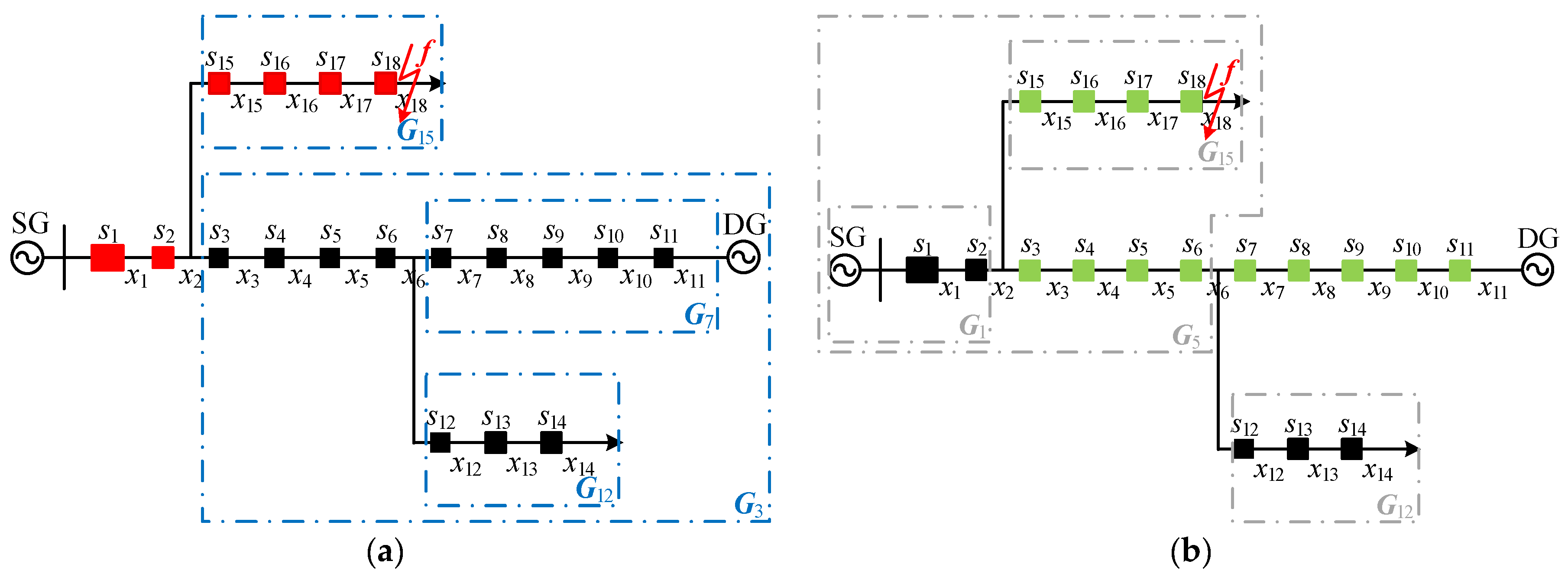
For a subnetwork that does not contain a T-type section (e.g., the subnetwork ${\mathit{G}}_7$, ${\mathit{G}}_{12}$, ${\mathit{G}}_{15}$ shown in Figure 3), no recursion is required, and its fault candidate set consists of the section with the largest value of the approximation gain in that network, as described in Theorem 8.

Theorem 8. 

Let ${\mathit{G}}_i=({\mathit{V}}_i,{\mathit{E}}_i)$ be a subnetwork that does not contain a T-type section, and suppose $x_k\in {\mathit{E}}_i$; if, $\forall x_r\ne x_k\in {\mathit{E}}_i$, there is always ${\Delta }_k>{\Delta }_r$, then the fault section set ${\mathit{X}}_i=\left\{x_k\right\}$ is the fault candidate set for ${\mathit{G}}_i$.

The proof of Theorem 8 is given in Appendix D.

3.2.3. Recursive Case

For a subnetwork containing a T-type section (e.g., subnetwork ${\mathit{G}}_3$ shown in Figure 3), a recursive solution is required. Its fault candidate set is constructed from the fault candidate set of a subnetwork smaller than its size, as described in Theorem 9.

Theorem 9. 

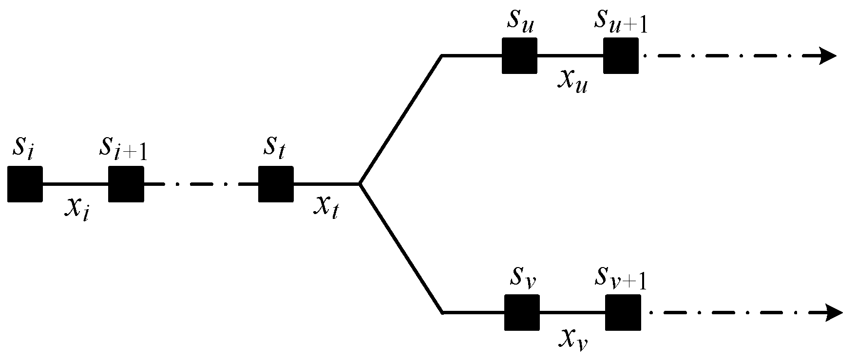
Let the subnetwork ${\mathit{G}}_i=({\mathit{V}}_i,{\mathit{E}}_i)$ contain T-type sections, and let section $x_t$ be the T-type section in ${\mathit{G}}_i$ that is closest to the main power supply, assuming that xu and xv are the downstream sections of $x_t$, as shown in Figure 4. Let ${\mathit{G}}_u=({\mathit{V}}_u,{\mathit{E}}_u)$and ${\mathit{G}}_v=({\mathit{V}}_v,{\mathit{E}}_v)$ be subnetworks and set ${\mathit{E}}_{i-t}={\mathit{E}}_i-{\mathit{E}}_u-{\mathit{E}}_v$. Suppose that for section $x_k\in {\mathit{E}}_{i-t}$, and  $\forall x_q\ne x_k\in {\mathit{E}}_{i-t}$, there is always ${\Delta }_k>{\Delta }_q$. Let ${\mathit{X}}_{i-t}=\left\{x_k\right\}$, and let its corresponding approximation gain be ${\Delta }_{{\mathit{X}}_{i-t}}={\Delta }_k$. Suppose that ${\mathit{X}}_u$ and ${\mathit{X}}_v$ are the fault candidate sets for subnetworks ${\mathit{G}}_u$ and ${\mathit{G}}_v$ respectively, and construct the set ${\mathit{X}}_{u\&v}={\mathit{X}}_u\cup {\mathit{X}}_v$. Let ${\Delta }_{{\mathit{X}}_{i-t}}$,  ${\Delta }_{{\mathit{X}}_u}$,  ${\Delta }_{{\mathit{X}}_v}$, and ${\Delta }_{{\mathit{X}}_{u\&v}}$ be the approximation gains of sets ${\mathit{X}}_{i-t}$, ${\mathit{X}}_u$,${\mathit{X}}_v$, and ${\mathit{X}}_{u\&v}$ respectively. Then, the set corresponding to the largest of ${\Delta }_{{\mathit{X}}_{i-t}}$, ${\Delta }_{{\mathit{X}}_u}$, ${\Delta }_{{\mathit{X}}_v}$, and ${\Delta }_{{\mathit{X}}_{u\&v}}$ is the fault candidate set ${\mathit{X}}_i$ of ${\mathit{G}}_i$.

The distribution network shown in Figure 3 is taken as an example to illustrate the meaning of Theorem 9. Subnetwork ${\mathit{G}}_3$ contains T-type section $x_6$. The fault location result of this network is constructed from the fault candidate sets of subnetworks ${\mathit{G}}_7$ and ${\mathit{G}}_{12}$, which are smaller than its size. Let the fault candidate sets of ${\mathit{G}}_7$ and ${\mathit{G}}_{12}$ be ${\mathit{X}}_7$ and ${\mathit{X}}_{12}$; their corresponding approximation gains are ${\Delta }_{{\mathit{X}}_7}$ and ${\Delta }_{{\mathit{X}}_{12}}$. Assume that the maximum approximation gain section found in the set of sections ${\mathit{E}}_{3-6}={\mathit{E}}_3-{\mathit{E}}_7-{\mathit{E}}_{12}=\{x_3,x_4,x_5,x_6\}$ is $x_k$; construct the set ${\mathit{X}}_{3-6}=\left\{x_k\right\}$, and its corresponding approximation gain is ${\Delta }_{{\mathit{X}}_{{}_{3-6}}}={\Delta }_k$. The set ${\mathit{X}}_{7\&12}={\mathit{X}}_7\cup {\mathit{X}}_{12}$ is constructed, and its corresponding approximation gain is ${\Delta }_{{\mathit{X}}_{7\&12}}$. Then, the set corresponding to the largest of ${\Delta }_{{\mathit{X}}_{{}_{3-6}}}$, ${\Delta }_{{\mathit{X}}_7}$, ${\Delta }_{{\mathit{X}}_{12}}$, and ${\Delta }_{{\mathit{X}}_{7\&12}}$ is the fault location result of ${\mathit{G}}_3$.

The proof of Theorem 9 is given in Appendix D.

4. Fault Section Location Method for Distribution Networks Based on Divide-and-Conquer

In the previous section, we demonstrate the recursive structure of the numerical model for fault location. In this section, we propose a fault location algorithm based on DAC and analyze the computational efficiency of the algorithm.

4.1. Algorithm Design

The fault location method closely follows the divide-and-conquer paradigm. Intuitively, it operates as follows.

• Divide. Divide the distribution network into smaller subnetworks using the T-type section closest to the main power source as the boundary (the decomposition effect is shown in Figure 4).
• Conquer. Recursively invoke the algorithm to solve the fault candidate set of the subnetwork. If the subnetwork no longer contains a T-type section, the recursion is stopped, and the fault candidate set is constructed directly according to Theorem 8.
• Combine. Combine the fault candidate set of subnetworks to create the fault candidate set of the original network according to Theorem 9.

The topological information of the network is the basis of the fault location for the distribution network, and the method of determining the topological information required by the algorithm is described below.

• Node number and section number. By applying the depth-first search algorithm, the section is traversed with the main power supply as the source node, and the sections are numbered in the order they are accessed so that the section numbers of any subnetwork in the network are consecutive and conform to the numbering rules in this paper.
• Section type vector T. Construct the section type vector T to determine the type of the section. When x_k is a T-type section, let T(k) = 1; otherwise, T(k) = 0.
• Adjacency list(Adj). Construct the adjacency list of the section to record the downstream section of each section for a fast search of the adjacency section of the T-type section, which helps implement the “divide” step in the recursive case.

When the distribution network topology changes, this operation is re-executed to make the algorithm flexible to adapt to the topology change.

The pseudocode DACFL gives the implementation of applying DAC to solve the subnetwork ${\mathit{G}}_i$ fault candidate set. Because the subnetwork section numbers are consecutive, the diagnostic range is determined by the starting section number i and the maximum section number j. DACFL accepts i, j, network topology information Graph (containing adjacency list and section type vector T), and the fault information vector I reported by FTUs as input. The fault candidate set X and its approximation gain ${\Delta }_{\mathit{X}}$ are returned. As described in Section 3.2.1, the distribution network fault location problem can be solved by solving the fault candidate set ${\mathit{X}}_1$ of its subnetwork ${\mathit{G}}_1$. Therefore, the algorithm initially set i = 1 and j to take the maximum number of the distribution network sections. The pseudocode for the algorithm is shown as Algorithm 1.

Algorithm 1 DACFL (i, j, Gragh, I, D)

1: $k=i$

2: ${\Delta }_k=D+2\mathit{I}(k)-1$

3: while $\mathit{T}(k)\ne 0$ and ${\Delta }_k=D+2\mathit{I}(k)-1$ do

4:  $k=k+1$

5:  ${\Delta }_k=D+2\mathit{I}(k)-1$

6: end while

7: if $k=j$ then                           // base case

8:  return (FIND-MAX ($\Delta [i:j]$))

9: end if

10: $ui=Adj(k)(1)$                        // divide

11: $vi=Adj(k)(1)$

12: if $ui>vi$ then

13:  $uj=j$

14:  $vj=ui-1$

15: else then

16:  $vj=j$

17:  $uj=vi-1$

18: end if

19: $({\mathit{X}}_u,{\Delta }_{{\mathit{X}}_u})=\mathrm{DACFL}(ui,uj,\mathrm{Graph},\mathit{I},{\Delta }_k)$          // conquer

20: $({\mathit{X}}_v,{\Delta }_{{\mathit{X}}_v})=\mathrm{DACFL}(vi,vj,\mathrm{Graph},\mathit{I},{\Delta }_k)$

21: $({\mathit{X}}_{i-t},{\Delta }_{{\mathit{X}}_{i-t}})=\mathrm{FIND}-\mathrm{MAX}(\Delta [i:k])$           // combine

22: ${\mathit{X}}_{u\&v}={\mathit{X}}_u\cup {\mathit{X}}_v$

23: ${\Delta }_{{\mathit{X}}_{u\&v}}={\Delta }_{{\mathit{X}}_u}+{\Delta }_{{\mathit{X}}_v}-{\Delta }_k$

24: if ${\Delta }_{{\mathit{X}}_u}=\max ({\Delta }_{{\mathit{X}}_{i-t}},{\Delta }_{{\mathit{X}}_u},{\Delta }_{{\mathit{X}}_v},{\Delta }_{{\mathit{X}}_{u\&v}})$ then

25:  return (${\mathit{X}}_u,{\Delta }_{{\mathit{X}}_u}$)

26: elseif ${\Delta }_{{\mathit{X}}_v}=\max ({\Delta }_{{\mathit{X}}_{i-t}},{\Delta }_{{\mathit{X}}_u},{\Delta }_{{\mathit{X}}_v},{\Delta }_{{\mathit{X}}_{u\&v}})$ then

27:  return (${\mathit{X}}_v,{\Delta }_{{\mathit{X}}_v}$)

28: elseif ${\Delta }_{{\mathit{X}}_{i-t}}=\max ({\Delta }_{{\mathit{X}}_{i-t}},{\Delta }_{{\mathit{X}}_u},{\Delta }_{{\mathit{X}}_v},{\Delta }_{{\mathit{X}}_{u\&v}})$ then

29:  return (${\mathit{X}}_{i-t},{\Delta }_{{\mathit{X}}_{i-t}}$)

30: else then

31:  return (${\mathit{X}}_{u\&v},{\Delta }_{{\mathit{X}}_{u\&v}}$)

32: end if

In detail, the DACFL procedure works as follows. Lines 1~2 of DACFL set the initial pointer position and calculate the approximation gain of the starting section, where the value of D is 0 when the algorithm is started, and the approximation gain of the upstream T-type section of the starting section xi is taken at each recursion thereafter (the calculation of the approximation gain of section x_k in lines 2 and 5 is described in the last paragraph of this section). Lines 3~6 traverse the section from the starting section x_i, determine whether there is a T-type section in ${\mathit{G}}_i$, and complete the calculation of the approximation gain of the T-type section and its upstream section. If ${\mathit{G}}_i$ does not contain a T-type section, the traversal process is not interrupted and ends with k = j. Otherwise, the process ends with k recording the T-type section number in ${\mathit{G}}_i$ that has the shortest distance from the main power supply.

Lines 7~9 correspond to the base case, where ${\mathit{G}}_i$ does not contain a T-type section. According to Theorem 8, the algorithm returns the section with the largest approximation gain as the location result at this time. Among them, the subroutine FIND-MAX returns the position and value of the largest element in the array.

Lines 10~32 correspond to the recursive case of ${\mathit{G}}_i$ containing T-type sections. Lines 10~17 are the “Divide” steps that determine the diagnostic range of the subnetwork ${\mathit{G}}_u$ and ${\mathit{G}}_v$. Lines 10~11 identify the starting section x_ui and x_vi of ${\mathit{G}}_u$ and ${\mathit{G}}_v$ from the adjacency list of section x_k. Because the section numbers are consecutive, lines 12~18 find the sections x_uj and x_vj with the largest number in ${\mathit{G}}_u$ and ${\mathit{G}}_v$ by comparing the sizes of ui and vi. Lines 19~20 are the “Conquer” steps, which recursively invoke the algorithm to find the fault candidate sets ${\mathit{X}}_u$, ${\mathit{X}}_v$ of ${\mathit{G}}_u$, ${\mathit{G}}_v$ and their approximation gains ${\Delta }_{{\mathit{X}}_u}$, ${\Delta }_{{\mathit{X}}_v}$. Lines 21~32 are the “Combine” steps. Line 21 finds the section with the largest approximation gain in the set of sections ${\mathit{E}}_{i-t}$ to form ${\mathit{X}}_{i-t}$ and its approximation gains ${\Delta }_{{\mathit{X}}_{i-t}}$. Lines 22~23 construct ${\mathit{X}}_{u\&v}$ and calculate ${\Delta }_{{\mathit{X}}_{u\&v}}$. Lines 24~32 find largest one from ${\Delta }_{{\mathit{X}}_{i-t}}$, ${\Delta }_{{\mathit{X}}_u}$, ${\Delta }_{{\mathit{X}}_v}$, ${\Delta }_{{\mathit{X}}_{u\&v}}$ and return its corresponding X and $\Delta$ as the result of the fault location for ${\mathit{G}}_i$.

In summary, the flow chart of the algorithm in this paper is shown in Figure 5.

It should be noted that Formulas (32) and (33) calculating the approximation gains ${\Delta }_k$ and ${\Delta }_{{\mathit{X}}_{u\&v}}$ have a linear time operation cost. To improve computational efficiency, lines 2, 5, and 23 of the algorithm use constant time operations to calculate ${\Delta }_k$ and ${\Delta }_{{\mathit{X}}_{u\&v}}$. The correctness of this calculation method is demonstrated in Appendix E and Appendix F.

4.2. Efficiency Analysis

To theoretically prove that the algorithm can satisfy the requirement of fault location speed, this section describes application of the time complexity of the aggregation analysis algorithm pseudocode to argue the computational efficiency of the algorithm.

Lines 1~2 of DACFL set the initial pointer position and calculate the approximation gain of the starting section, which will be executed once in each recursion. Lines 3~6 traverse the sections of the distribution network, each of which takes constant time. The process will be interrupted by the appearance of T-type sections but can be continued in the subnetworks G_u and G_v. According to aggregation analysis, lines 3~5 are executed once for each section of the distribution network. Line 7 determines the subnetwork type, executed once at each recursion. Line 8 and lines 10~32 correspond to the base and recursive cases, respectively, and are executed once per recursion at most. Each line takes constant time, except for lines 8 and 21. Lines 8 and 21 find the maximum value from the values of j − i + 1 and k − i + 1. Line 8 is executed for the base case. Line 21 is executed for the recursive case containing T-sections, but the same will be continued in the next recursion. Applying aggregation analysis, eventually, the approximation gain of each section will be taken out and compared once; thus, the overall number of operations in lines 8 and 21 is the number of sections in the distribution network.

Let the distribution network contain n nodes, and the number of algorithm recursions is l. “Progressive notation” is applied to represent the operation cost and total running time of each line [32], and the analysis results of this algorithm efficiency are summarized in

Table 4. Efficiency analysis.

Steps	Number of Executions	Operation Cost	f(X)
Lines 1~2	l	Θ(1)	Θ(l)
Lines 3~5	n	Θ(1)	Θ(n)
Line 6~7	l	Θ(1)	Θ(l)
Lines 8, 21	< l	Θ(j-i) or Θ(k-i)	Θ(n)
Line 9	l	Θ(1)	Θ(l)
Lines 10~20	< l	Θ(1)	O(l)
Lines 22~32	< l	Θ(1)	O(l)

.

According to the “Divide” step of the pseudocode DACFL, the number of recursions depends on the number of downstream sections of the T-type sections in the distribution network; thus, l < n. Combining the analysis results of Table 4, the time complexity of DACFL is

$$\Theta (l)+\Theta (n)+\Theta (l)+\Theta (n)+\Theta (l)+O(l)+O(l)=\Theta (n)$$

(34)

It can be seen that the pseudocode DACFL has a linear level of time complexity, thereby proving the efficient computational capability of the algorithm in this paper. It can be foreseen that the method proposed in this section has great potential for improving the computational efficiency of fault location in the context of large-scale distribution networks.

4.3. Active Distribution Network Application Note

For active distribution networks containing distributed generations (DGs), the short-circuit current after a fault will flow in both directions, and then, the encoding of fault information described in Equation (1) would no longer applicable. In this paper, we refer to the sections that reach the substation power supply through node s_i as the downstream sections of node s_i and the remaining sections in the distribution network as the upstream sections of node s_i. The fault information of node s_i is determined by Equation (35) [33].

$${\mathit{J}}_i(\mathit{X})=\left\{{\displaystyle \prod _{{\mathit{G}}_u}^{}\left[K_{{\mathit{G}}_u}\left(1-{\displaystyle \prod _{x_{\mathit{G}u}\in {\mathit{E}}_{i,{\mathit{G}}_u}}{y}_{\mathit{G}u}}\right)\right]}\right\}{\displaystyle \prod _{x_d\in {\mathit{E}}_{i,d}}^{}{y}_d}-\left\{{\displaystyle \prod _{{\mathit{G}}_d}^{}\left[K_{{\mathit{G}}_d}\left(1-{\displaystyle \prod _{x_{\mathit{G}d}\in {\mathit{E}}_{i,{\mathit{G}}_d}}{y}_{\mathit{G}d}}\right)\right]}\right\}{\displaystyle \prod _{x_u\in {\mathit{E}}_{i,u}}^{}{y}_u}$$

(35)

where G_u denotes the power source connected to the upstream section of node s_i, which is referred to as the upstream power source of node si. $K_{{\mathit{G}}_u}$ denotes the throw-off factor of G_u, when G_u is put into operation $K_{{\mathit{G}}_u}=1$; otherwise, $K_{{\mathit{G}}_u}=0$. $y_{\mathit{G}u}$ denotes the operating state of the feeder section $x_{\mathit{G}u}$ between s_i and G_u. In contrast, G_d, $K_{{\mathit{G}}_d}$, and $y_{\mathit{G}d}$ denote the variables associated with the downstream power supply of node s_i. G_d denotes the downstream power supply of s_i, $K_{{\mathit{G}}_d}$ denotes the throw-off factor of G_d, and $y_{\mathit{G}d}$ denotes the operating state of the feeder section $x_{\mathit{G}d}$ between s_i and G_d. In addition, $y_d$ and $y_u$ indicate the operation status of the downstream section of and the upstream section of s_i, respectively, and “$\prod$” indicates the logical “OR” superposition operation.

In Equation (35), it can be seen that each grid-connected power source will only provide fault current in a single direction to the node after a distribution network fault, and the fault state of the node can be regarded as the superposition of the states under the action of each power source individually. Therefore, the coding rule of node s_i to grid-connected power sources S is proposed as

$${\mathit{I}}_{i,S}=\left\{\begin{array}{ll}1& \mathrm{Short} \mathrm{circuit} \mathrm{current} \mathrm{is} \mathrm{detected} \mathrm{in} \mathrm{the} \mathrm{same} \mathrm{direction} \\ & \mathrm{as} \mathrm{the} \mathrm{short} \mathrm{circuit} \mathrm{current} \mathrm{supplied} \mathrm{by} \mathrm{power} \mathrm{supply} \mathrm{S}\\ 0& \hspace{1em}\hspace{1em}\hspace{1em}\hspace{1em}\hspace{1em}\mathrm{Others}\end{array}\right.$$

(36)

Meanwhile, because the road from the section to each power source is unique, the distribution network with each power source as the main power source has a radial structure. In view of this, the following fault section location process for an active distribution network based on DAC is proposed.

• Step 1: Store the network topology information (including node section number, adjacency list, and section type vector T) of the distribution network with each power source as the main power source.
• Step 2: After the failure of the distribution network, take the grid-connected power supply as the main power supply, and the corresponding network topology information and node fault information vector determined by Equation (36) are taken as the input. The fault candidate sets X of each power supply as the main power supply are determined by the fetching algorithm.
• Step 3: The fault candidate sets X obtained from Step 2 is combined to obtain the final fault location result.

4.4. Fault Location Case

To understand the fault location process of the method in this paper, this section selects various types of fault examples to elaborate on the operation process of the algorithm.

4.4.1. Test Case 1: Single Fault

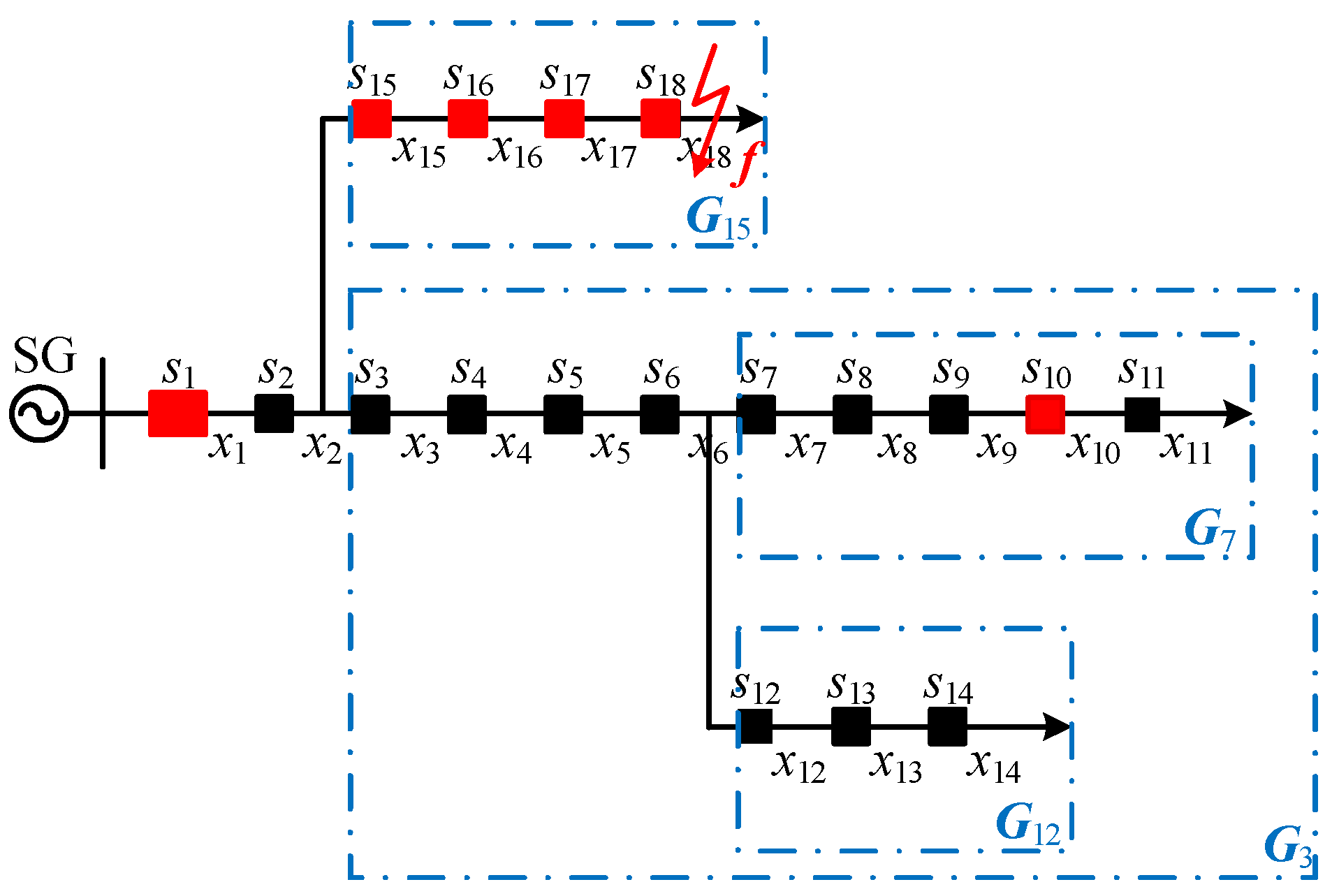
In Figure 6, assume that section x₉ in the multi-branch distribution network has a fault. The nodes that detect the fault current report the fault information, which is marked with red boxes.

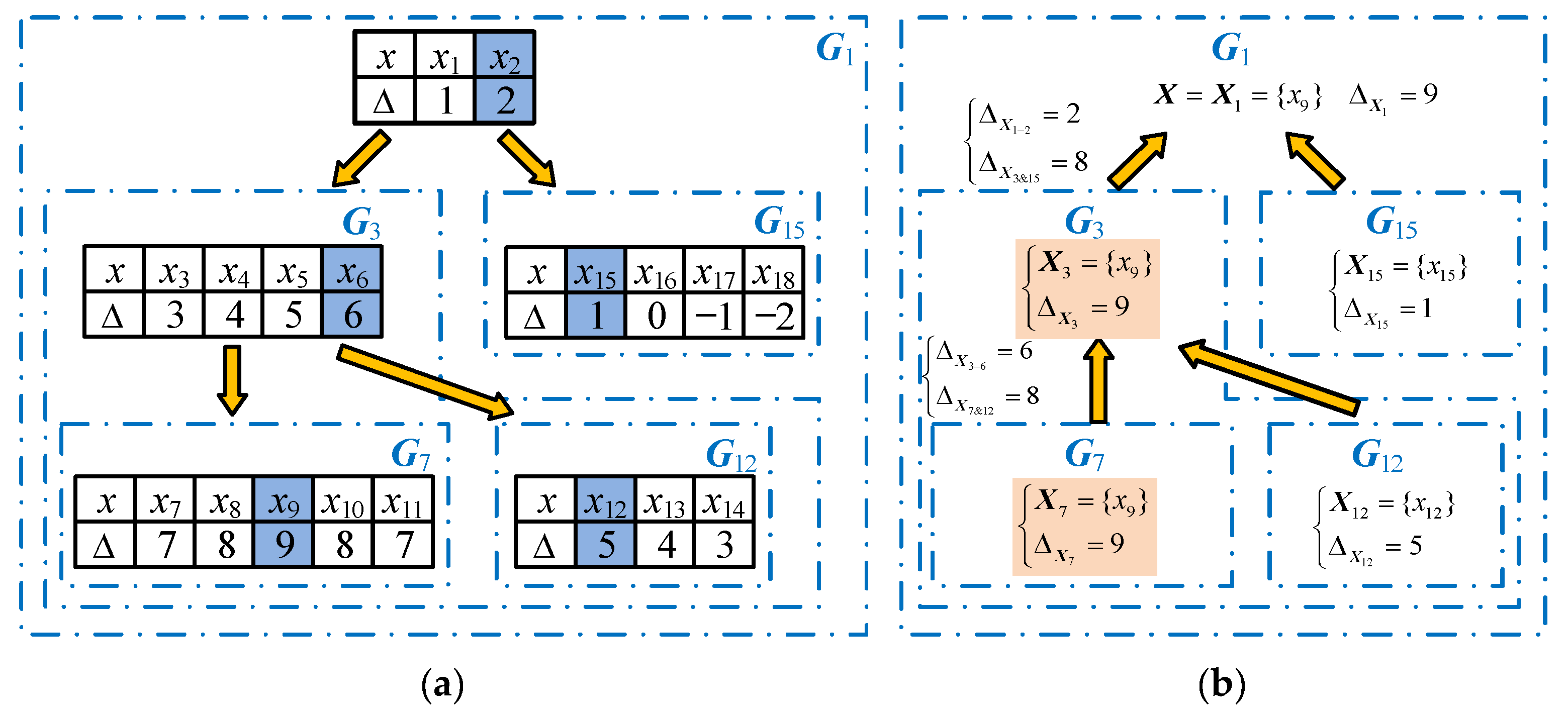
The algorithm traverses the sections in the network from the starting section x₁, calculates the approximation gain of the sections, and determines the section’s type. When accessing section x₂, x₂ is detected as a T-type section, and the network is divided into subnetwork ${\mathit{G}}_3$ and subnetwork ${\mathit{G}}_{15}$. The algorithm is called recursively for ${\mathit{G}}_{15}$, and when the traversal end k = 18 ${\mathit{G}}_{15}$ is determined to be the base case that does not contain a T-type section. The section with the maximum approximation gain in x₁₅~x₁₈ is x₁₅. According to Theorem 8, ${\mathit{X}}_{15}=\left\{x_{15}\right\}$ and ${\Delta }_{{\mathit{X}}_{15}}={\Delta }_{15}=1$ are taken as the fault location results of ${\mathit{G}}_{15}$. Call the algorithm recursively for ${\mathit{G}}_3$, traverse the sections in ${\mathit{G}}_3$ from x₃, detect that x₆ is a T-type section, and divide the network into ${\mathit{G}}_7$ and ${\mathit{G}}_{12}$. Call the algorithm recursively for ${\mathit{G}}_7$, and when the traversal end k = 11, determine ${\mathit{G}}_7$ as the base case and return the result of fault location: ${\mathit{X}}_7=\left\{x_9\right\}$, ${\Delta }_{{\mathit{X}}_7}={\Delta }_9= 9$. Similarly, ${\mathit{X}}_{12}=\left\{x_{12}\right\}$ and ${\Delta }_{{\mathit{X}}_{12}}={\Delta }_{12}= 5$ are taken as the fault location results of ${\mathit{G}}_{12}$. The divide process of the algorithm and the calculation results of each section approximation gain are shown in Figure 7a.

The combine process of the algorithm is shown in Figure 7b, and the detailed running procedure is as follows. Combine the fault candidate sets ${\mathit{G}}_3$ and ${\mathit{G}}_{12}$ to create the fault location result ${\mathit{G}}_3$. Find the section x₆ with the largest approximation gain from x₃ to x₆ and construct the set of sections ${\mathit{X}}_{3-6}=\left\{x_6\right\}$ with the approximation gain ${\Delta }_{{\mathit{X}}_{3-6}}={\Delta }_6=6$. Construct the set ${\mathit{X}}_{7\&12}={\mathit{X}}_7\cup {\mathit{X}}_{12}=\{x_9,x_{12}\}$, whose approximation gain is ${\Delta }_{{\mathit{X}}_{7\&12}}=8$. The largest approximation gain of ${\Delta }_{{\mathit{X}}_{3-6}}$, ${\Delta }_{{\mathit{X}}_7}$, ${\Delta }_{{\mathit{X}}_{12}}$, and ${\Delta }_{{\mathit{X}}_{7\&12}}$ is ${\Delta }_{{\mathit{X}}_7}$; thus, ${\mathit{X}}_7$ and ${\Delta }_{{\mathit{X}}_7}$ are taken as the fault location results of ${\mathit{G}}_3$, i.e., ${\mathit{X}}_3={\mathit{X}}_7=\left\{x_9\right\}$, ${\Delta }_{{\mathit{X}}_3}={\Delta }_{{\mathit{X}}_7}= 9$. Combine the fault candidate sets of ${\mathit{G}}_3$ and ${\mathit{G}}_{15}$ to create the fault location result ${\mathit{G}}_1$. Find the section x₂ with the largest approximation gain from x₁ to x₂ and construct the set of sections ${\mathit{X}}_{1-2}=\left\{x_2\right\}$ with the approximation gain ${\Delta }_{{\mathit{X}}_{1-2}}={\Delta }_2= 2$. Construct the set ${\mathit{X}}_{3\&15}={\mathit{X}}_3\cup {\mathit{X}}_{15}=\{x_9,x_{15}\}$, whose approximation gain is ${\Delta }_{{\mathit{X}}_{3\&15}}=8$. The largest approximation gain of ${\Delta }_{{\mathit{X}}_{1-2}}$, ${\Delta }_{{\mathit{X}}_3}$, ${\Delta }_{{\mathit{X}}_{15}}$, and ${\Delta }_{{\mathit{X}}_{3\&15}}$ is ${\Delta }_{{\mathit{X}}_3}$; thus, ${\mathit{X}}_3$ and ${\Delta }_{{\mathit{X}}_3}$ are taken as the fault location results of ${\mathit{G}}_1$, i.e., ${\mathit{X}}_1={\mathit{X}}_3=\left\{x_9\right\}$, ${\Delta }_{{\mathit{X}}_1}={\Delta }_{{\mathit{X}}_3}= 9$. The algorithm is executed, and x₉ is determined to be the fault section.

4.4.2. Test Case 2: Multiple Faults

In Figure 8, assume that both sections x₉ and x₁₈ have a fault simultaneously. The nodes that reported the fault information are marked with red boxes.

The divide process of the algorithm is similar to that of Test Case 1. The divide process of the algorithm and the calculation results of each section approximation gain are shown in Figure 9a.

The combine process of the algorithm is shown in Figure 9b, and the detailed running procedure is as follows. Combine the fault candidate sets ${\mathit{G}}_7$ and ${\mathit{G}}_{12}$ to create the fault location result ${\mathit{G}}_3$. Find the section x₆ with the largest approximation gain from x₃ to x₆ and construct the set of sections ${\mathit{X}}_{3-6}=\left\{x_6\right\}$ with the approximation gain ${\Delta }_{{\mathit{X}}_{3-6}}={\Delta }_6=6$. Construct the set ${\mathit{X}}_{7\&12}={\mathit{X}}_7\cup {\mathit{X}}_{12}=\{x_9,x_{12}\}$, whose approximation gain is ${\Delta }_{{\mathit{X}}_{7\&12}}=8$. The largest approximation gain of ${\Delta }_{{\mathit{X}}_{3-6}}$, ${\Delta }_{{\mathit{X}}_7}$, ${\Delta }_{{\mathit{X}}_{12}}$, and ${\Delta }_{{\mathit{X}}_{7\&12}}$ is ${\Delta }_{{\mathit{X}}_7}$; thus, ${\mathit{X}}_7$ and ${\Delta }_{{\mathit{X}}_7}$ are taken as the fault location results of ${\mathit{G}}_3$, i.e., ${\mathit{X}}_3={\mathit{X}}_7=\left\{x_9\right\}$, ${\Delta }_{{\mathit{X}}_3}={\Delta }_{{\mathit{X}}_7}= 9$. Combine the fault candidate sets ${\mathit{G}}_3$ and ${\mathit{G}}_{15}$ to create the fault location result ${\mathit{G}}_1$. Find section x₂ with the largest approximation gain from x₁ to x₂ and construct the set of sections ${\mathit{X}}_{1-2}=\left\{x_2\right\}$ with the approximation gain ${\Delta }_{{\mathit{X}}_{1-2}}={\Delta }_2= 2$. Construct the set ${\mathit{X}}_{3\&15}={\mathit{X}}_3\cup {\mathit{X}}_{15}=\{x_9,x_{15}\}$, whose approximation gain is ${\Delta }_{{\mathit{X}}_{3\&15}}=13$. The largest approximation gain of ${\Delta }_{{\mathit{X}}_{1-2}}$, ${\Delta }_{{\mathit{X}}_3}$, ${\Delta }_{{\mathit{X}}_{15}}$, and ${\Delta }_{{\mathit{X}}_{3\&15}}$ is ${\Delta }_{{\mathit{X}}_{3\&15}}$; thus, ${\mathit{X}}_{3\&15}$ and ${\Delta }_{{\mathit{X}}_{3\&15}}$ are taken as the fault location results of ${\mathit{G}}_1$, i.e., ${\mathit{X}}_1={\mathit{X}}_{3\&15}=\{x_9,x_{18}\}$, ${\Delta }_{{\mathit{X}}_1}={\Delta }_{{\mathit{X}}_{3\&15}}=13$. After the algorithm is executed, x₉ and x₁₈ are determined to be the fault sections.

4.4.3. Test Case 3: Fault Information Distortion

In actual projects, FTUs are mostly installed outdoors, where the working environments are harsh and the reported fault information may be misreported, missed, or experiencing other distortions. Therefore, it should be possible to output correct positioning results as much as possible in the case of small-scale distortion of information. This case sets up the small-scale distortion of information to test the information fault tolerance of the algorithm.

In Figure 10, assume that section x₁₈ has a fault. Node s₁₀ misreports the fault information (i.e., I₁₀: 0 → 1), and node s₂ misses the fault information (i.e., I₂: 1 → 0). The nodes that reported the fault information are marked with red boxes.

The divide process of the algorithm is similar to Test Case 1. The divide process of the algorithm and the calculation results of each section approximation gain are shown in Figure 11a.

The combine process of the algorithm is shown in Figure 11b, and the detailed running procedure is as follows. Combine the fault candidate sets ${\mathit{G}}_7$ and ${\mathit{G}}_{12}$ to create the fault location result ${\mathit{G}}_3$. Find the section x₃ with the largest approximation gain from x₃ to x₆ and construct the set of sections ${\mathit{X}}_{3-6}=\left\{x_3\right\}$ with the approximation gain ${\Delta }_{{\mathit{X}}_{3-6}}={\Delta }_3=-1$. Construct the set ${\mathit{X}}_{7\&12}={\mathit{X}}_7\cup {\mathit{X}}_{12}=\{x_7,x_{12}\}$, whose approximation gain is ${\Delta }_{{\mathit{X}}_{7\&12}}=-6$. The largest approximation gain of ${\Delta }_{{\mathit{X}}_{3-6}}$, ${\Delta }_{{\mathit{X}}_7}$, ${\Delta }_{{\mathit{X}}_{12}}$, and ${\Delta }_{{\mathit{X}}_{7\&12}}$ is ${\Delta }_{{\mathit{X}}_{3-6}}$; thus, ${\mathit{X}}_{3-6}$ and ${\Delta }_{{\mathit{X}}_{3-6}}$ are taken as the fault location results of ${\mathit{G}}_3$, i.e., ${\mathit{X}}_3={\mathit{X}}_{3-6}=\left\{x_3\right\}$, ${\Delta }_{{\mathit{X}}_3}={\Delta }_{{\mathit{X}}_{3-6}}=-1$. Combine the fault candidate sets ${\mathit{G}}_3$ and ${\mathit{G}}_{15}$ to create the fault location result ${\mathit{G}}_1$. Find the section x₁ with the largest approximation gain from x₁ to x₂ and construct the set of sections ${\mathit{X}}_{1-2}=\left\{x_1\right\}$ with the approximation gain ${\Delta }_{{\mathit{X}}_{1-2}}={\Delta }_1= 1$. Construct the set ${\mathit{X}}_{3\&15}={\mathit{X}}_3\cup {\mathit{X}}_{15}=\{x_9,x_{15}\}$, whose approximation gain is ${\Delta }_{{\mathit{X}}_{3\&15}}= 3$. The largest approximation gain of ${\Delta }_{{\mathit{X}}_{1-2}}$, ${\Delta }_{{\mathit{X}}_3}$, ${\Delta }_{{\mathit{X}}_{15}}$, and ${\Delta }_{{\mathit{X}}_{3\&15}}$ is ${\Delta }_{{\mathit{X}}_{15}}$; thus, ${\mathit{X}}_{15}$ and ${\Delta }_{{\mathit{X}}_{15}}$ are taken as the fault location results of ${\mathit{G}}_1$, i.e., ${\mathit{X}}_1={\mathit{X}}_{15}=\left\{x_{18}\right\}$, ${\Delta }_{{\mathit{X}}_1}={\Delta }_{{\mathit{X}}_{15}}= 4$. After the algorithm is executed, x₁₈ is determined to be the fault section.

As can be seen from Test Case 3, the algorithm proposed in this paper uses the redundancy of fault information in the whole network to tolerate the distorted information, which can accurately locate the fault with small-scale distortion of fault information.

4.4.4. Test Case 4: Active Distribution Network

In Figure 12, assume that section x₁₈ in the active distribution network has a fault. SG and DG are the main power sources, respectively, and the corresponding nodes’ fault information is marked in red and green boxes in Figure 12a and Figure 12b, respectively.

The call algorithm determines the result of fault location with each power supply as the main power supply, and the algorithm’s divide process and combine process are shown in Figure 13.

In Figure 13, it can be seen that the result of fault location with SG and DG as the main power source are ${\mathit{X}}_1= \{x_{18}\}$, ${\mathit{X}}_{11}= \{x_{18}\}$, respectively. The final location result is obtained by taking the two together: $\mathit{X}={\mathit{X}}_1\cup {\mathit{X}}_{11}= \{x_{18}\}$. After the algorithm is executed, x₁₈ is determined to be the fault section.

5. Simulation Analysis

In order to test the performance of the proposed method, this section describes, taking the IEEE 33-node power distribution system and IEEE 69-node power distribution system as examples, fault location simulation tests performed on the MATLAB simulation environment on an Intel Core i7-1260P CPU 4.70GHz platform, and the results are compared with the current typical fault location algorithms in terms of accuracy, fault tolerance, and computational efficiency. The compared algorithms include the binary particle swarm optimization algorithm (Algorithm 2) [20], bald eagle search algorithm (Algorithm 3) [31], and linear integer programming algorithm (Algorithm 4) [26]. The specific fault location methods for each algorithm are shown in

Table 5. Fault location methods for various algorithms.

Algorithm Number	Algorithm Type	Fault Location Method
Algorithm 1	Algorithm in this paper	Algorithm in this paper. Construct a numerical computational model for fault location with the help of road vector, and apply DAC to locate the fault.
Algorithm 2	Intelligent optimization algorithm	Assuming all possible fault scenarios in the distribution network, construct a solution space and apply the binary particle swarm optimization algorithm to locate the fault section in the solution space.
Algorithm 3	Hierarchical fault location algorithm	Partition the distribution network according to the branch structure, apply the bald eagle search algorithm to locate the fault branch first, and then determine the fault section by applying the exhaustive method in the fault branch.
Algorithm 4	Linear integer programming algorithm	Construct a linear integer programming model for fault location using ascending dimension and apply the branch and bound method to locate the fault.

.

5.1. IEEE 33-Node Distribution Network

The IEEE 33-node distribution system is shown in Figure 14, which has 1 substation power supply, 1 circuit breaker, 32 intelligent switches, and 33 sections. The population size of the intelligent optimization algorithm was set to 50, and the maximum number of iterations was set to 30.

5.1.1. Accuracy

To test the accuracy of the algorithm, it was run 100 times with multiple fault types, such as single faults, multiple faults, and end-of-supply faults. The accuracy of the algorithm is described by the ratio of the number of correct locations to the total number of runs. The test results are shown in

Table 6. Accuracy test results.

Equipment Number	Preset Fault Section	Accuracy (%)
		Algorithm 1	Algorithm 2	Algorithm 3	Algorithm 4
1	x8	100	94	99	100
2	x26	100	80	100	100
3	x28	100	82	100	100
4	x30	100	78	99	100
5	x4, x29	100	96	100	100
6	x11, x28	100	84	96	100
7	x25, x30	100	81	100	100
8	x6, x27	100	95	100	100

.

As can be seen in Table 6, all four algorithms have correct result outputs; the difference lies in their ability to maintain consistency in their results. Algorithm 2 and Algorithm 3 cannot guarantee 100% accuracy. The accuracy of Algorithm 2 is around 85%, which is due to the fact that the algorithm applies an intelligent algorithm with stochastic search characteristics to locate faults, and along with the depth of iterations, the population tends to homogenize, leading to possible local convergence; thus, the consistency of results cannot be guaranteed. Algorithm 3 applies a hierarchical strategy to reduce the fault search dimension, and its accuracy is improved, but it still needs to locate the fault branch with the help of an intelligent algorithm; thus, the defect of insufficient convergence stability cannot be eradicated. With the pseudocode DACFL, the algorithm in this paper does not contain random operations, which makes the algorithm have the same execution process for the same fault situation; thus, it can guarantee consistency in its results. The test results confirm that Algorithm 1 achieved 100% accuracy for the fault cases in Table 6.

5.1.2. Fault Tolerance

In actual engineering, the distortion of fault information reported by FTU is divided into two cases of misreporting or omission of the reported information. Omission of the reported information refers to the fault current exceeding the set threshold and the FTU not reporting the fault information. Misreporting means that the FTU reports fault information, but the actual situation does not match it.

In this section, different numbers and locations of false alarm and omission signals are set to simulate a variety of information distortion situations in real projects to test the information tolerance of the algorithm.

As can be seen in

Table 7. Fault tolerance test results.

Equipment Number	Preset Fault Section	Preset Information Distortion	Accuracy (%)
			Algorithm 1	Algorithm 2	Algorithm 3	Algorithm 4
1	x3	I16: 0 → 1	100	84	100	100
2	x18	I7: 1 → 0, I32: 0 → 1	100	80	Misjudgment	100
3	x23	I4: 1 → 0	100	88	100	100
4	x33	I11: 0 → 1, I20: 0 → 1	100	86	99	100
5	x7, x22	I14: 1 → 0	100	90	100	100
6	x10, x33	I6: 1 → 0, I30: 1 → 0	100	70	98	100
7	x16, x27	I7: 1 → 0, I22: 0 → 1, I32: 0 → 1	100	76	Misjudgment	100
8	x14, x26	I10: 1 → 0	100	72	100	100

, the accuracy of Algorithm 2 dropped to about 80%. Algorithm 3 requires high information reliability of the branch nodes and therefore produced misjudgment for fault cases 2 and 7, in which the branch nodes were distorted. The fault location model of the algorithm in this paper was derived using strict mathematical derivation and is fully equivalent to the classical localization model, which is fault-tolerant to distorted information with the help of redundancy of fault information in the whole network. The test results confirm that Algorithm 1 had 100% accuracy for the fault information distortion case in Table 7.

5.1.3. Computational Efficiency

The algorithms were run 100 times, and the average time consumed by the algorithms was taken as a measure of computational efficiency. The test results are shown in

Table 8. Computational efficiency test results.

Equipment Number	Preset Fault Section	Preset Information Distortion	Computational Efficiency (ms)
			Algorithm 1	Algorithm 2	Algorithm 3	Algorithm 4
1	x18		13.27	131.43	75.27	118.18
2	x24	I9: 0 → 1, I20: 1 → 0	13.86	128.29	79.34	116.76
3	x6	I12: 0 → 1	15.16	128.45	77.98	126.72
4	x33	I2: 1 → 0	16.85	129.23	76.25	142.61
5	x11, x20	I8: 1 → 0, I29: 0 → 1	14.33	133.67	103.56	121.98
6	x17, x33	I22: 0 → 1	13.46	128.92	109.54	130.47
7	x4, x29		15.32	133.96	108.48	152.42
8	x12, x23	I5: 1 → 0, I8: 1 → 0, I15: 0 → 1	15.05	149.75	106.26	112.01

.

From Table 8, it can be seen that the computational efficiency of Algorithm 2 was around 130 ms, which is due to the fact that the algorithm needs to perform iterative operations in a high-dimensional solution space. Algorithm 3 applies a hierarchical strategy to reduce the fault search dimension, and its computational efficiency was around 90 ms. Algorithm 4 had a computational efficiency of about 127 ms. The analysis in Section 4.2 confirms that the algorithm proposed in this paper has a linear level of time complexity. The test results show that the computational efficiency of Algorithm 1 was below 20 ms, which is a significant advantage compared with the other three algorithms.

5.2. IEEE 69-Node Distribution Network

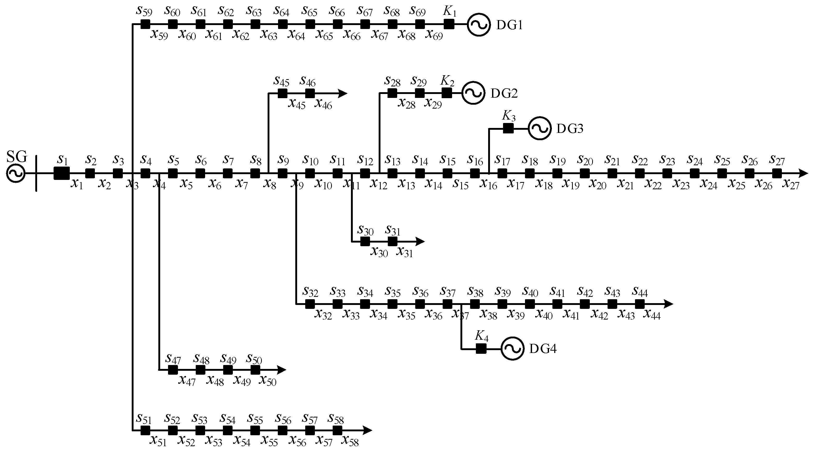
The IEEE 69-node distribution system is shown in Figure 15, which has 1 substation power supply, 4 distributed power supplies, 1 circuit breaker, 4 DG grid-connected switches, 68 intelligent switches, and 69 sections. The population size of the intelligent optimization algorithm was set to 100, and the maximum number of iterations was set to 70.

To further demonstrate the performance advantages of the proposed method, this section describes taking the IEEE69-node distribution system as an example to test the accuracy and computational efficiency of the algorithms. The test cases in this section are shown in

Table 9. Test cases for IEEE 69-node distribution network.

Equipment Number	[K1, K2, K3, K4]	Preset Fault Section	Preset Information Distortion
1	[1, 1, 1, 1]	x52	I8: −1 → 0
2	[0, 1, 1, 1]	x15	I49: 0 → 1
3	[1, 1, 1, 1]	x57	I20: 0 → −1, I51: 1 → 0
4	[1, 0, 1, 1]	x16, x32	I8: 1 → 0, I25: 0 → 1, I39: 0 → −1
5	[0, 1, 1, 1]	x64
6	[1, 1, 0, 1]	x10, x36	I15: 0 → −1
7	[1, 1, 1, 0]	x12, x35	I7: 1 → 0, I32: 1 → 0, I41: 0 → −1
8	[1, 1, 1, 1]	x56, x67	I35: −1 → 0, I63: 1 → −1
9	[1, 1, 1, 1]	x14, x23	I17: 1 → 0, I34: −1 → 1, I43: 0 → 1
10	[1, 1, 1, 1]	x9, x59	I24: 0 → 1, I63: −1 → 0
11	[1, 0, 0, 1]	x27, x34
12	[1, 0, 1, 1]	x7	I34: −1 → 1, I62: −1 → 0

, which covers various fault scenarios such as single-fault, multiple-fault, sound fault information, and distorted fault information. Among them, the application vectors K₁, K₂, K₃, and K₄ represent the dynamic throwing cases of the distributed power supply. When DGi is put into operation, K_i = 1; otherwise, K_i = 0.

5.2.1. Accuracy

As the size of the network increases, the solution space of the fault location problem increases, which causes an intelligent algorithm with randomized search operations to be more prone to local convergence. As can be seen in Figure 16a, the accuracy of Algorithm 2 dropped below 50% for some of the test cases. The accuracy of Algorithm 3 was higher than that of Algorithm 2, but it produced misjudgment for fault cases 3, 7, and 9, where the branch nodes were distorted. As mentioned previously, the algorithm in this paper does not contain random operation and makes use of the redundancy of fault information in the whole network to tolerate the distorted information; thus, its accuracy was almost not affected by the network size. The test results confirm that Algorithm 1 maintained an accuracy of 100% for the various fault cases, as seen in Table 9.

5.2.2. Computational Efficiency

From Figure 16b, it can be seen that the computational efficiency of Algorithm 1 was below 50 ms for a 69-node scale distribution network, thanks to its linear time complexity, which indicates that the advantage of the computational efficiency of the algorithm proposed in this paper is more obvious in large distribution networks. For the intelligent optimization algorithm represented by Algorithm 2, the population size of the algorithm is usually no less than the number of sections of the distribution network to ensure the correct rate. Assuming that the distribution network contains n sections, Algorithm 2 needs to operate on at least n individuals in the iterative process, and the cost of individual operation is $\Theta (n)$. Even with the convergence condition of “no update of global extremum” [20], the asymptotic lower bound of $\Omega (n^2)$ is available in the best case. The test results show that the computational efficiency of Algorithm 2 was around 400 ms, which is more than eight times different from the algorithm in this paper. The fault area determination process of Algorithm 3 still requires iterative operations, and its section location requires exhaustive fault scenarios, which affects location speed. The test results show that the computational efficiency of Algorithm 3 was about 200 ms, which is more than four times different from the algorithm in this paper. The solution of Algorithm 4 involves the computation of its continuous relaxation LP model several times, and the time complexity of the LP problem reached O(n⁴) [27]. From Figure 16b, we can see that the algorithm had the lowest computational efficiency, which reached the second level and had a large gap compared with the computational efficiency of the algorithm in this paper.

5.3. Comparative Analysis of Performance

In summary,

Table 10. Comparative results of algorithm performance.

Algorithm Number	Algorithm Type	Accuracy	Computational Efficiency
Algorithm 1	Algorithm in this paper	Highest	Highest
Algorithm 2	Intelligent optimization algorithm	Low	Low
Algorithm 3	Hierarchical fault location algorithm	Higher	Higher
Algorithm 4	Linear integer programming algorithm	Highest	Lowest

gives a comparison of the results of the algorithms’ performance.

In terms of accuracy, as described in Section 5.1.1, all of the algorithms in the comparison output correct localization results, but the difference lies in their ability to maintain the consistency of their output results during repeated testing. In other words, the accuracy of the algorithms is closely related to the convergence stability. The intelligent optimization algorithm represented by Algorithm 2 has a random population generation and update, and the population form tends to be homogeneous with the depth of iteration; thus, it sometimes converges to the “local extreme value point” in the process of repeated testing, and it cannot maintain consistency in its output results. When the scale of distribution network is expanded, the scale of solution space increases, and these problems become more prominent. The hierarchical fault location algorithm, represented by Algorithm 3, uses a hierarchical strategy to reduce the size of the solution space and improve the convergence stability. However, this algorithm only uses the FTU information of the branch port in determining the fault area, which may lead to misjudgment when the FTU information of the port is distorted. The linear integer programming algorithm, represented by Algorithm 4, applies the classical integer programming algorithm to locate faults, in which the “optimality check” step can make it gradually bound through iteration and eventually converge to the same “global optimal solution”; thus, it has higher convergence stability. From the pseudocode DASFL in Section 4.1, we can see that the algorithm proposed in this paper does not contain random operations and has the same execution process and calculation results in the same fault situation; thus, it can maintain the consistency of the results, which makes the algorithm of this paper have high convergence stability.

The computational efficiency of the algorithm was determined using the time complexity of the algorithm. Assuming that the distribution network contains n sections, as described in Section 5.2.2, Algorithm 4 had a time complexity of O(n⁴), and therefore has the lowest computational efficiency. Algorithm 2 requires iterative search operations in a high-dimensional solution space. If it adopts the convergence condition of “no update at the global extremum”, it ideally has the asymptotic lower bound of $\Omega (n^2)$, and in the extreme case, the number of iterations of Algorithm 2 is the maximum number of iterations, at which time the algorithm has the asymptotic upper bound of $O(n^3)$. Therefore, its computational efficiency is higher than that of Algorithm 4. Algorithm 3 applies a hierarchical strategy to transform the single-layer, high-dimensional search operation into a double-layer, low-dimensional search operation; thus, its computational efficiency is higher than that of Algorithm 2. As described in Section 4.2, the algorithm in this paper has a linear level of time complexity $\Theta (n)$, and it therefore has the highest computational efficiency.

6. Conclusions

The existing distribution network fault section location model contains a large number of logic operations and does not meet the requirements of rapidity and accuracy of fault diagnosis. Therefore, a fault location method based on divide-and-conquer is proposed in this paper. In addition, through a simulated test, the following conclusions can be drawn.

• DAC reduces the operational dimension of fault location to have a linear level of time complexity, which improves the computational efficiency of fault location more significantly. The test results show that for distribution networks with a scale of 33 and 69 nodes, the computational efficiency of the algorithm in this paper is below 20 ms and 50 ms, respectively, which is more than eight times faster than the traditional intelligent optimization algorithms.
• The algorithm in this paper does not contain random search operation; thus, it has strong numerical stability. The test results show that the accuracy of the algorithm in this paper is not affected by the size of the network, and it is more than 19.25% higher than the traditional intelligent optimization algorithm.
• The numerical calculation model of fault location proposed in this paper uses the redundancy of fault information in the whole network to tolerate the distorted information, which can accurately locate the fault with a small amount of distortion in the fault information.

This paper was based on the fault alarm information uploaded by FTU to locate distribution network faults, which has the advantages of clear and simple information link and convenient implementation. However, when the amount of fault information distortion exceeds the acceptable amount of redundancy, misjudgment could occur. Future research could be conducted on the fault criterion of multi-source information fusion to further improve the accuracy of distribution network fault location.

References

1. Li, G.; Chen, Q.; Zhang, J. Novel faulted section location method for distribution network based on status information of fault indicating equipment. Appl. Sci. 2020, 10, 5910. [Google Scholar] [CrossRef]
2. He, W.; Wang, S.; Xu, T.; Shen, H.; Su, Y.; Liu, Z.; Xiong, Z.; Wang, X. A construction and development path of the urban resilient distribution network. Power Syst. Technol. 2022, 46, 680–690. [Google Scholar]
3. Galvez, C.; Abur, A. Fault location in active distribution networks containing distributed energy resources (DERs). IEEE Trans. Power Deliv. 2021, 36, 3128–3139. [Google Scholar] [CrossRef]
4. Zhao, F.; Meng, Z.; Li, Y.; Liu, C. Pilot protection scheme for active distribution network based on fault components. High Volt. Eng. 2019, 45, 3092–3100. [Google Scholar]
5. Wang, S.; Liu, Q.; Zhao, Q.; Wang, H. Connotation Analysis and Prospect of Distribution Network Elasticity. Autom. Electr. Power Syst. 2021, 45, 1–9. [Google Scholar]
6. Shen, G.; Zhang, Y.; Qiu, H.; Wang, C.; Wen, F.; Salam, M.; Weng, L.; Zhang, L.; Zhang, S. Fault diagnosis with false and/or missing alarms in distribution systems with distributed generators. Energies 2018, 11, 2579. [Google Scholar] [CrossRef]
7. Wang, S.; Song, L.; Shu, X. Adaptive overcurrent protection of active distribution network with high penetration of distributed generations and multiple loads. High Volt. Eng. 2019, 45, 1783–1794. [Google Scholar]
8. Zheng, T.; Ma, L.; Zhang, B. Fault tolerant fast fault section location method for active distribution network. J. N. China Electr. Power Univ. 2022, 49, 12–20. [Google Scholar]
9. Zhao, Q. Research on Wide Area Protection of Smart Distribution Grid; North China Electric Power University: Beijing, China, 2017. [Google Scholar]
10. Xu, B.; Yin, X.; Zhang, Z.; Pang, S.; Li, X. Fault location for distribution network based on matrix algorithm and optimization algorithm. Autom. Electr. Power Syst. 2019, 43, 152–158. [Google Scholar]
11. Ji, X.; Zhang, S.; Zhang, Y.; Han, X.; Xiao, Y.; Zeng, R. Fault section location for distribution network based on improved electromagnetism-like mechanism algorithm. Autom. Electr. Power Syst. 2021, 45, 157–165. [Google Scholar]
12. Teng, J.; Huang, W.; Luan, S. Automatic and fast faulted line-section location method for distribution systems based on fault indicators. IEEE Trans. Power Syst. 2014, 4, 1653–1662. [Google Scholar] [CrossRef]
13. Ma, T.; Gao, L. Fault location algorithm for active distribution network with multi micro-grids. Power Syst. Prot. Control 2017, 45, 64–68. [Google Scholar]
14. Wang, Q.; Jin, T.; Mohamed, A. A fast and robust fault section location method for power distribution systems considering multisource information. IEEE Syst. J. 2022, 16, 1954–1964. [Google Scholar] [CrossRef]
15. Jiao, Y.; Du, S.; Wang, Q.; Chen, C. Information aberrance correction and fault-section location for distribution networks based on the information contradiction theory. Power Syst. Prot. Control 2014, 42, 43–48. [Google Scholar]
16. Zheng, T.; Ma, L.; Li, B. Fault section location of active distribution network based on feeder terminal unit information distortion correction. Power Syst. Technol. 2021, 45, 3926–3934. [Google Scholar]
17. Kong, B.; Liu, J.; Zhou, J.; Zhou, Y.; Song, Z. Fault-tolerant algorithm for fault location in distribution network based on integer linear programming. Power Syst. Prot. Control 2020, 48, 27–35. [Google Scholar]
18. Wei, Z.; He, H.; Zheng, Y. A refined genetic algorithm for the fault sections location. Proc. CSEE 2002, 22, 127–130. [Google Scholar]
19. Guo, Z.; Chen, B.; Liu, C.; Xu, K.; Li, J. Fault location of distribution network based on genetic algorithm. Power Syst. Technol. 2007, 31, 88–92. [Google Scholar]
20. Zhao, Q.; Wang, Z.; Dong, W.; Bao, W. Research on fault location in a distribution network based on an immune binary particle swarm algorithm. Power Syst. Prot. Control 2020, 48, 83–89. [Google Scholar]
21. Zhang, Y.; Zhou, R.; Zhong, K. Application of improved ant colony algorithm in fault-section location of complex distribution network. Power Syst. Technol. 2011, 35, 224–228. [Google Scholar]
22. Liu, B.; Wang, F.; Chen, C.; Huang, H.; Dong, X. Harmony search algorithm for solving fault location in distribution networks with DG. Trans. China Electrotech. Soc. 2013, 28, 280–284. [Google Scholar]
23. Wang, Q.; Jin, T.; Tan, H.; Zhu, S.; Liu, S. A complete analytic model of section location in distribution network based on multi-factor dimensionality deduction. Trans. China Electrotech. Soc. 2019, 34, 3012–3024. [Google Scholar]
24. Guo, Z.; Xu, Q.; Hong, J.; Mao, X. Integer linear programming based fault section diagnosis method with high fault-tolerance and fast performance for distribution network. Proc. CSEE 2017, 37, 786–795. [Google Scholar]
25. He, R.; Hu, Z.; Li, Y.; Wang, T. Fault section location method for DG-DNs based on integer linear programming. Power Syst. Technol. 2018, 42, 3684–3690. [Google Scholar]
26. Li, Z.; Wang, Z.; Zhang, Y.; Qiao, X. Fault section location method for active distribution network based on linear programming with ascending dimension. Autom. Electr. Power Syst. 2021, 12, 122–131. [Google Scholar]
27. Yin, Y.; Wang, D.; Yu, Y. Integer Programming, 1st ed.; Science Press: Beijing, China, 2022; pp. 56–66. [Google Scholar]
28. Wang, Q.; Jin, T.; Tan, H.; Li, Z. The technology on fault location of distribution network based on hierarchical model and intelligent checking algorithm. Trans. China Electrotech. Soc. 2018, 33, 5327–5337. [Google Scholar]
29. Zheng, C.; Zhou, H.; Zheng, D.; Lin, Z.; Zhang, X. An active distribution network fault location method based on improved multi-universe algorithm. Power Syst. Prot. Control 2023, 51, 169–179. [Google Scholar]
30. Gao, F.Y.; Li, Z.J.; Yuan, C.; Qi, X.D.; Li, X.F.; Zhuang, S.X. Fault location for active distribution network based on quantum computing and immune optimization algorithm. High Volt. Eng. 2021, 47, 396–406. [Google Scholar]
31. Yang, G.; Feng, J.; Liu, X.; Chen, R.; Pan, H.; Yang, Q. Fault location of a distribution network hierarchical model with a distribution generator based on IBES. Power Syst. Prot. Control 2022, 50, 1–9. [Google Scholar]
32. Cormen, T.H.; Leiserson, C.E.; Rivest, R.L.; Stein, C. Introduction to Algorithms, 3rd ed.; The MIT Press: London, UK, 2009; pp. 24–37. [Google Scholar]
33. Li, Y.; Wang, Z.; Zhao, Q. Distributed fault section location for ADN based on bayesian complete analytic model and multi-factor dimension reduction. Power Syst. Technol. 2021, 45, 3917–3925. [Google Scholar]
Figure 1. The basic working principle of the fault location method based on FTUs.
Applsci 13 05974 g001
Figure 2. Typical active distribution network.
Applsci 13 05974 g002
Figure 3. Multi-branch distribution network.
Applsci 13 05974 g003
Figure 4. Subnetwork with T-type section.
Applsci 13 05974 g004
Figure 5. Flowchart of the algorithm.
Applsci 13 05974 g005
Figure 6. Single fault in the multi-branch distribution network.
Applsci 13 05974 g006
Figure 7. The execution process of the algorithm under a single fault. (a) Divide process; (b) combine process.
Applsci 13 05974 g007
Figure 8. Multiple faults in the multi-branch distribution network.
Applsci 13 05974 g008
Figure 9. Execution process of the algorithm under multiple failures. (a) Divide process; (b) combine process.
Applsci 13 05974 g009
Figure 10. Fault information distortion in the multi-branch distribution network.
Applsci 13 05974 g010
Figure 11. Execution process of the algorithm under fault information distortion. (a) Divide process; (b) combine process.
Applsci 13 05974 g011
Figure 12. Multiple faults in the multi-branch active distribution network. (a) Fault information of SG as the main power source; (b) fault information of DG as the main power source.
Applsci 13 05974 g012
Figure 13. The execution process of the algorithm in an active distribution network. (a) Divide process with SG as the main power source; (b) combine process with SG as the main power source; (c) divide process with DG as the main power source; (d) combine process with DG as the main power source.
Applsci 13 05974 g013
Figure 14. IEEE 33-node distribution system.
Applsci 13 05974 g014
Figure 15. IEEE 69-node distribution system.
Applsci 13 05974 g015
Figure 16. The test results of the IEEE 69-node distribution system. (a) Accuracy comparison; (b) comparison of computational efficiency.
Applsci 13 05974 g016