Abstract
Reconstructing 3D models from a single image has numerous applications in fields such as VR/AR, medical imaging, and gaming. However, most mesh-based methods are limited by the use of 0-genus initial templates, which makes it difficult to reconstruct 3D meshes with complex topologies. Additionally, existing methods often prioritize reconstructing the overall shape and neglect to study local meshes with varying curvatures, resulting in a lack of correct and detailed local features in the generated meshes. This paper proposes a 3D reconstruction framework that transitions from global to local and incorporates MLP and GCN. The framework introduces a mesh pruning strategy under a 2D hole constraint to restore the correct mesh topology. Moreover, the framework fine-tunes local details by separately learning corresponding mapping functions on high-frequency and low-frequency local extended patches. The experiment with the proposed network on the ShapeNet dataset shows that the network has a CD value of 1.763 and an F-score of 85.40. The results from extensive experiments demonstrate that our proposed method outperforms existing methods in topology correction and local detail reconstruction.
1. Introduction
Reconstructing the 3D structure of an object from a single image is an important task in computer vision and graphics. However, due to the ill-posed nature of single-view 3D reconstruction, additional prior knowledge or appropriate constraints are required to restore the correct 3D shape of an object. In recent years, the development of deep learning and the popularization of 3D shape datasets [1,2,3] have enabled neural networks to encode the hidden structural information of images effectively, resulting in significant advancements in the field of 3D reconstruction.
Existing research on single-view reconstruction employs various 3D shape representations, including implicit functions [4,5,6,7], voxels [8,9,10,11], point clouds [12,13,14], meshes [15,16,17,18,19,20,21,22,23], and others. Voxel-based methods are challenging to reconstruct high-precision shapes due to the large amount of memory and computational time required to apply 3D CNN. The point cloud representation lacks connection information between points, making it difficult to represent the surface details of 3D objects. Methods based on implicit functions often require the execution of expensive post-processing steps, such as the Marching cube algorithm [24], to generate functional 3D structures. Compared with other representations, the mesh adopted in this paper is a compact, seamless, and coherent surface representation capable of representing finer surface details with smaller data sizes.
However, methods using mesh representation face significant challenges:
The first challenge is dealing with objects with complex topological structures. Most mesh-based single-view reconstruction methods mainly rely on the free deformation of the initial mesh, which limits the reconstruction to meshes with 0-genus topology. According to topology theory [25], the topological properties of meshes remain unchanged under homeomorphic morphism. As shown in Figure 1, the reconstruction results of the mesh-based method [16] are topologically equivalent to the 0-genus initial template, and the lack of correct holes in the reconstruction results has become a shortcoming that affects the visual effect. Recent studies [18] have begun to explore mesh pruning to generate corresponding holes by estimating the sampling point error; however, smaller holes cannot be handled due to the sparseness of the sampling point cloud. Moreover, data-driven methods have difficulty recovering uncommon holes in the dataset. Thus, achieving the correct topology of the reconstruction result remains a significant problem in the field.
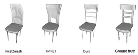
Figure 1.
The first challenge for single-view reconstruction.
The second challenge of mesh reconstruction is the difficulty of generating smooth surfaces with precise details. As shown in Figure 2, the plane lacks sufficient detail in the high-curvature wing parts to reconstruct the engine, and the lower-curvature parts, such as the fuselage, are not smooth enough when compared to the ground truth. This issue can be explained in terms of frequency: the high-curvature part of the mesh contains a large number of high-frequency features, while the high-frequency information in the low-curvature part is mainly noise. Thus, the neural network should retain the high-frequency signal as much as possible in the high-curvature part while suppressing the high-frequency information in the low-curvature part. However, existing methods do not differentiate between high- and low-curvature meshes, which may lead to the worst-case scenario of lacking detail in high-curvature and too much noise in low-curvature.
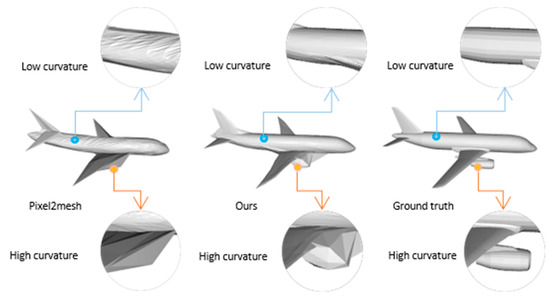
Figure 2.
The second challenge for single-view reconstruction.
In order to address these challenges, we propose a framework for global-to-local single-view mesh reconstruction that can independently fine-tune high-frequency and low-frequency local meshes and introduce 2D hole constraints to restore the correct mesh topology. First, a structure that incorporates multilayer perceptron (MLP) and graph convolutional neural networks (GCN) can reduce the number of graph neural network (GNN) layers by restoring the global shape of the mesh using cascaded MLP deformation blocks, thereby reducing memory consumption and over-smoothing issues [26]. At the same time, we believe that the 2D image contains the whole information in the corresponding view. On the basis of this assumption, we employ a novel mesh pruning strategy constrained by 2D holes to restore the correct mesh topology during the global shape recovery stage. Another key idea of this paper is to use an extended patch extract module to make the framework transition naturally from global to local, and then design a dual-branch refinement block composed of FAGCN [27] to fine-tune the high-frequency and low-frequency parts. The dual-branch local refinement structure can adaptively utilize features of different frequencies so that the high-curvature branch can utilize maximally high-frequency information while the low-curvature branch suppresses high-frequency features. To ensure the visual effect of the local mesh, we simultaneously design a local loss suitable for optimization on the local patch. Finally, quantitative and qualitative experiments demonstrate that the proposed method outperforms existing methods.
The contributions of this paper can be summarized as follows:
- We propose a framework for single-view mesh reconstruction that transitions from global to local, combining the advantages of MLP and GNN and mitigating the over-smoothing caused by deep GNN.
- We propose a new strategy for mesh pruning under the constraint of 2D holes that overcomes the limitation of the 0-genus template by combining hole contour information from 2D images to perform adaptive mesh topology correction.
- We facilitate fine-tuning of parts with different curvatures by separating the high- and low-frequency parts of the mesh and learning the corresponding mapping functions on the local extension patches of the high and low frequencies.
- We designed a series of experiments to demonstrate the superiority of the proposed method in topology correction and detail reconstruction over the existing methods.
2. Related Work
Contrary to methods that employ multi-view stereo geometry [28,29,30,31], single-view 3D reconstruction is an ill-posed problem and still faces many challenges. With the success of deep learning, a large body of literature began to study the use of deep learning to reconstruct 3D objects from a single colorful image. Existing deep learning-based single-view 3D reconstruction methods can be categorized into four types based on their decoder output representation: implicit function representation [4,5,6,7], voxel representation [8,9,10,11], point cloud representation [12,13,14], and mesh representation [15,16,17,18,19,20,21,22]. In this section, we will conduct a literature review of these different methods.
2.1. Implicit Function Representation
The implicit function-based method [4,5,6,7] represents the object surface as a continuous field, enabling the generation of high-quality 3D forms. In order to make the object shape present excellent visual effects, Chen et al. [4] designed a binary classifier as the decoder to predict if a point is within the mesh. Different from Chen, Mescheder et al. [5] proposed an occupancy network to learn the continuous decision boundary, capable of generating high-resolution 3D meshes. Xu et al. [6] combined local and global features to predict the signed distance function, while the visual effect is better in regions that are thin or holey. Different from other methods, Chen et al. [7] subdivided the spatial hierarchy into multiple convex sets through binary space partitioning, which can well reconstruct structures such as sharp corners. Although methods using implicit function representation can produce precise shapes, these methods must perform expensive post-processing algorithms such as the marching cube algorithm [24] to extract meshes before they can be used in practical applications.
2.2. Voxel Representation
The voxel-based method [8,9,10,11] directly generates the voxel occupancy of 3D space. 3D-R2N2 [8] used a 3D recurrent neural network to unify the correspondence between single and multiple images into 3D voxels. In [10], a differentiable ray consistency term was proposed to improve single-view reconstruction tasks. Wu et al. [11] introduced shape priors to overcome 2d-to-3d ambiguity. However, the expensive memory requirements and computation time of 3D CNN limit the resolution of reconstruction results. A recent study [9] proposed using the octree structure to reduce the memory occupation of 3D convolution to a certain extent; however, it still could not achieve a satisfactory resolution.
2.3. Point Cloud Representation
As a simple and popular explicit representation method, point clouds have been widely used in many fields. Fan et al. [12] were the first to demonstrate the potential and expressiveness of point clouds. Jiang et al. [13] further introduced a geometric adversarial loss to improve the expressiveness of point clouds. Contrary to other methods, Zhao et al. [14] proposed a coarse-to-fine framework to generate high-fidelity point clouds. However, despite the advantages of simplicity, flexibility, and small memory, point clouds lack the ability to capture the connectivity between points and therefore cannot generate smooth and continuous surfaces.
2.4. Mesh Representation
The mesh representation has been widely used due to its ability to represent fine surface details at smaller data scales. Most existing mesh-based methods rely on mesh deformation techniques. Jack et al. [15] proposed a method that recovers 3D objects from a single image by deforming a template mesh. Pixel2mesh [16] reconstructed meshes from a single RGB image by using the graph unpooling layer from coarse to fine. Different from previous methods, Geometrics [19] improved the fine-grained details of meshes by using adaptive subdivision and zero-neighbor GCN. In [32], an effective adversarial domain confusion method was proposed to solve the pose-disentangled problem. Yi et al. [22] proposed a novel visual attention-guided network called Vanet, which handles the 3D reconstruction problem of single-view and multi-view simultaneously under a unified framework. However, these methods are limited by the topology of the initial template mesh, making it difficult to handle objects with complex topologies. To address this issue, Pan et al. [18] proposed an adaptive topology correction strategy to achieve correct topology. However, this method may be less effective for uncommon and small holes. Shi et al. [21] introduced mesh editing and a geometry structure extractor to facilitate mesh topology correction and improve fine-grained details. Tang et al. [20] improved the reconstruction of objects with complex topologies by adopting shape skeletons; however, their method cannot be trained end-to-end.
3. Method
In this chapter, we describe the complete pipeline for mesh reconstruction from a single image. Meanwhile, we detail the important components of the proposed method as well as its motivation.
3.1. Overview
Our goal is to recover smooth meshes with complex topology and fine details from a single RGBA image. In this paper, the mesh is represented as a graph , where is the set of N vertices of the mesh. is the set of directed edges connecting adjacent vertices, and is the set of faces of the mesh. We gradually fit the target surface S by deforming a 0-genus sphere mesh G0 by using a progressive structure, where the template G0 has 2562 vertices. Our pipeline is depicted in Figure 3, and we adopt an encode-decode architecture that transitions from global to local. The whole framework consists of the following five parts: image feature extractor, deformation block, pruning module, extend patch extract module and local refinement module. The image feature extractor maps the RGBA image I to the latent layer vector h, and the MLP-based global deformation block performs topological deformation on G0 to generate a coarse mesh. Notably, we use a mesh pruning module under 2D hole constraints during the global deformation stage to generate meshes with complex topologies. Next, we use an extended patch extract module to separate the coarse mesh into sets of high-curvature local patches and sets of low-curvature local patches . and represent the i-th high-curvature and i-th low-curvature patches, respectively. Meanwhile, the frame transitions from global shape recovery to local refinement. Finally, we utilize the dual-branch local refinement module to perform fine-tuning.
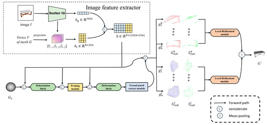
Figure 3.
The overall framework of the proposed method.
3.2. Image Feature Extractor
As shown in Figure 3, we employ ResNet-18 [33] to create an image feature extractor that accepts RGBA images as input and extracts 1024-dim global feature vectors . As a high-level semantic feature, contains the global shape information of the object to be reconstructed. In addition, we believe that shallow features contain more information, such as textures, which play an important role in recovering detail. Therefore, different from other methods [16,34], we use the camera parameters to project the mesh vertex coordinates to the shallow feature maps (f1_1, f2_2, f3_2) of ResNet-18 and calculate the bilinear interpolation on the feature map projection points to extract a 256-dim local feature vector . Finally, we concatenate and form a 1280-dim feature vector h.
3.3. Global Deformation Block
In some methods [16,29] of forming deformed blocks by graph convolution, we found that these methods often adopt a deep structure to obtain a relatively large receptive field, which causes the problem of over-smoothing [26,35,36] and hinders the generation of fine-grained mesh. Therefore, we choose to use the MLP deformation block similar to that used in Atlasnet [37] to generate a coarse mesh, which can reduce the number of layers in GCN. The global deformation block consists of five shared MLPs of sizes 1024, 512, 256, 128, and 3, with BN layers and ReLU on the first four layers and then activation on the output layer. We concatenate the vertex position V of the mesh G0 as a position encoding with the feature h to freely deform G0 using the global deformation block. In particular, we regress vertex coordinates in the first deformation block and vertex offsets in the second deformation block.
3.4. Pruning Module
In order to generate meshes with the correct topology, we prune the mesh under 2D hole constraints between the two deformation blocks. As shown in Figure 4a, the proposed estimator under the contour constraint takes G and the α channel of image I as input and returns the index of the pruning surface. Specifically, the estimator performs a boundary tracking algorithm [38] on the α channel of the input image I to detect the location of holes. Further, we use 0 to represent the non-hole area on the 2D plane and assign different values to the pixels at different hole positions to make the hole feature map. The estimator collects 2D hole features corresponding to V through a camera matrix and bilinear interpolation. Since the 2D hole constraint only works in the visible case, an error estimate module of TMNET [18] is introduced as a complement in the case where the holes are not visible. In order to save training time, we use the whole feature map of the corresponding view prepared in advance in actual training.
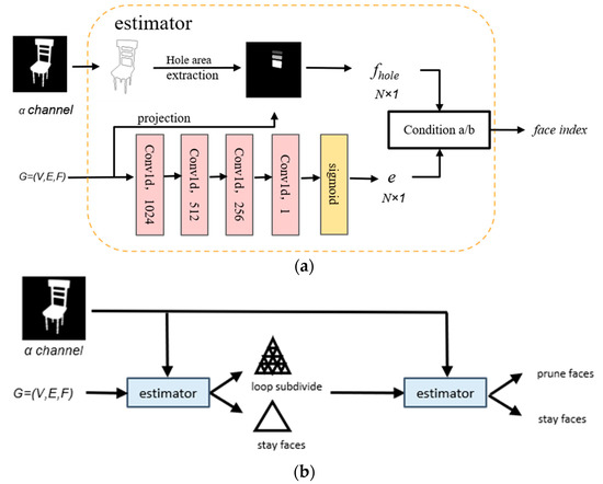
Figure 4.
Pruning module. (a) The framework of estimator. (b) The whole process of mesh pruning. The structure of the estimator under 2D hole constraints, where condition a is that e > τ or fhole > 0 of any point, and condition b is that the fhole of the three vertices of the face are equal and not 0 or e > τ.
The entire pruning procedure is depicted in Figure 4b. We noticed that the coarse meshes generated by the deformed blocks tended to be sparse in the hole region. Therefore, two loop subdivisions [39] are performed on the pruned surface to distinguish between pruned and unpruned regions. In order to locate the subdivision area, the first estimator uses the sampling point Vs as the input point and determines the subdivision face according to condition a (see Figure 4). To prevent erroneous pruning, the second estimator input point is the mesh vertex V, and the face to be pruned is determined according to condition b (see Figure 4). Our method improves robustness by introducing the hole contour constraint, which effectively handles holes with uncommon locations and small areas and requires only one pruning operation to achieve the desired effect.
3.5. Extend Patch Extract Module
Dividing the overall mesh into small local patches is beneficial for graph convolution to get rid of the influence of the features of distant irrelevant points, and the feature frequencies of high-curvature and low-curvature parts are different. Based on the above factors, we employ the extended patch extract module to generate local patch sets and to learn the local details of different curvatures.
Inputting the coarse mesh G generated in the previous stage, the extend patch extract module divides the mesh vertices into two seed point sets and according to the curvature Q and the farthest point sampling (Q > t1 is a high-curvature point, Q < t2 is a low-curvature point). As shown in Figure 5a, the extend patch extract module extracts the 5-hop neighborhood of the seed point as the basic patch , and further retains the one-way edge from the 6-hop point to the 5-hop point to form an extended patch , which can preserve the information of the connection and promote mesh smoothing. Finally, according to the patch of the nearest point from any point of the ground truth S to the Vs, we divided the corresponding and as the supervision of patches.
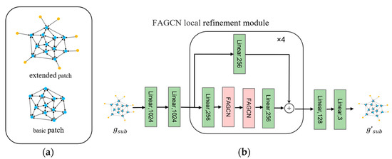
Figure 5.
Local refinement module. (a) the base patch and the extended patch; (b) the structure of the local refinement module.
3.6. Local Refinement Module
In this section, we employ a dual-branch structure consisting of the local refinement module to learn the corresponding fine-tuning mapping functions for high and low frequencies, respectively. Each local refinement module consists primarily of FAGCN [27] in order to allow the neural network to learn to adaptively filter parameters of different frequencies. The FAGCN operators are as follows:
In Equation (1), is the initial feature of node i, ldim is the dimension of the hidden layer, is the neighborhood of node i, di is the degree of node i, and ε is a scaling hyper-parameter limited to [0, 1]. Equation (2) shows the calculation method of the attention coefficient , where || represents the concatenation operation, and is a trainable parameter.
The structure of the local refinement module is shown in Figure 5b. Initially, we map 1283-dim features to 1024-dim features using two linear layers with ReLU. To avoid the negative effect caused by the entanglement of filters and weight matrices, we use a linear layer with ReLU before the FAGCN operator to convert the initial features to 256 dimensions. Multiple cascading filters may result in a narrow passband. Therefore, we add skip connections to ensure that the network can take advantage of features at various frequencies. Since we learn on small-scale local graphs, we use 4 residual blocks instead of a deeper GNN structure, which is sufficient to meet the requirements, thereby improving the over-smoothing issue caused by a too deep GNN. Finally, we use a linear layer of Tanh layers to output the offsets of vertex positions. The high and low curvature parts are treated differently by the two branches, resulting in different parameters learned by the two branches. The low-curvature branch learns a low-pass filter to filter noise and maintain smoothness, while the high-curvature branch learns a high-pass filter to restore details. Notably, the loss at the two branch ports is calculated during training, but during inference, the two types of patches are stitched to the original mesh using mean pooling, resulting in a smoother mesh seam.
3.7. Loss Function
The loss function used consists of two parts: a global loss and a local loss . In , we use chamfer distance as the primary loss function (see in [12]).
where and represent the set of points sampled from the generated mesh G and ground truth S, respectively.
In this paper, similar to TMNET, we utilize the L2 loss as to train the error estimation network [18]. In order to avoid severe self-intersection during the process of global deformation and to improve the mesh’s smoothness, we employ the commonly used geometric regularization term [16,40]. The normal loss is used to maintain the normal consistency between the generated mesh and the ground truth, and the smooth loss is used to maintain a smooth target surface. The edge loss is used to penalize overly long edges and prevent outliers.
The final global shape recovery loss is as follows:
We use local loss to fine-tune local patches. Different from , each item of is calculated on the subgraph and the corresponding ground truth. Note that the one-way edge of the extended patch is involved in the calculation of the regularization term to maintain the smoothness of the seam. In addition, we introduce a move loss to penalize the points with excessive offset.
where vi and vi′ are the vertices of subgraph g before and after fine-tuning, respectively.
The final local patch fine-tuning loss is as follows:
4. Result and Discussion
In this chapter, we evaluate the performance of the proposed method on the ShapeNet [1] dataset. In addition to comparing with the SOTA (state-of-the-art, SOTA) model, we evaluate the impact of individual components on the overall performance through ablation experiments. Finally, we extended the proposed method to real-world datasets.
4.1. Experiment Settings
Dataset. We evaluated the proposed method on 13 core classes of the ShapeNet [1] dataset. In this paper, we uniformly sampled 10,000 points on the surface of each CAD (computer-aided design, CAD) [1] model as the ground truth. For a fair comparison, we adopt the rendered images and corresponding camera parameters provided by Choy et al. [8]. The data of each class is divided into a training set, a validation set, and a test set according to the ratio of 70:10:20.
Train details. To improve training stability, we adopt the staged training approach of Pan et al. [18] to train each subnet separately and then fine-tune the entire network in an end-to-end manner. In this paper, all experiments are performed on a workstation with an Intel Xeon Gold 5218R CPU and an NVIDIA GTX 3090 GPU. We train the network using the Pytorch framework and the Adam optimizer [41] (β1 = 0.9, β2 = 0.999). The framework takes as input a 224 × 224 image I with a batch size of 32 and a spherical mesh G0 with 2562 vertices, and the number of local patches n = 8. We train for 300 epochs with a learning rate of 1 × 10⁻³ and decay to 1 × 10⁻⁴ after 100 epochs. The hyperparameter values are as follows: λ1 = 1 × 10⁻³, λ2 = 5 × 10⁻⁷, λ3 = 0.1, λ4 = 1 × 10⁻⁴. The pruning threshold τ is set to 0.02, the curvature hyperparameters of the extend patch extract module are set to t1 = 0.6, t2 = 0.2, and the scale ε of the FAGCN is set to 0.1. During training, the local patch refinement module directly uses the output patches to calculate the loss, while in the inference stage, the output patches are stitched to the overall mesh through mean pooling.
Evaluation Metric. In the paper, we evaluate the performance of the reconstruction results by the chamfer distance [12] and the F-score [42] with a threshold of 0.001, which is calculated between 10,000 sampling points in the generated mesh and the ground truth. The smaller the Chamfer Distance (CD) value, the better, and the larger the F-score, the better.
4.2. Comparisons with the State-of-the-Arts
In this section, we compare the proposed method with SOTA models, including Pixel2Mesh [16], Atlasnet [37], TMNET [18], and Vanet [22]. We measure the performance of the proposed method by calculating the chamfer distance and F-score. However, the existing quantitative indicators cannot fully reflect the reconstructed shape quality, so we demonstrate the advantages of the proposed method in detail recovery and topology correction by visualizing the reconstruction results.
Figure 6 demonstrates the visualization results. In this experiment, we aligned the output results uniformly. As can be seen from Figure 6, Pixel2Mesh and Vanet are incapable of reconstructing non-zero-genus objects and lack correct details in high-curvature parts, while low-curvature parts are not sufficiently smooth. The reconstruction results of Atlasnet suffer from severe self-intersection and cannot recover the correct topology (such as the hole in the chair back). Benefiting from the application of the mesh adaptive pruning strategy, TMNET can generate more complex topological structures; however, it is incapable of handling holes with a small surface area or infrequent locations. Our method can reconstruct more intricate topologies than TMNET and Atlasnet (such as holes in chairs, benches, and tables). Moreover, the large results of our method are smoother than those of other methods in areas with low curvatures, such as the chair’s seat surface and the monitor’s screen, and have more detail in the lamp’s areas with high curvature.
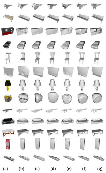
Figure 6.
Qualitative comparisons. (a) image, (b) Pixel2Mesh [16], (c) Atlasnet [37], (d) TMNET [18], (e) Vanet [22], (f) Ours, (g) Ground truth.
We compare the performance of the proposed method and SOTA models quantitatively. The results are shown in Table 1, and we use ∆ to denote the difference between the quantitative results of our method and TMNET. It should be noted that methods such as Pixel2Mesh reduce the shape by a factor of 0.57, which causes inconsistency between our quantitative results and those obtained by these methods. In terms of CD and F-score values, our method outperforms other methods in the majority of categories and averages, with average CD and F-scores that are 0.418 and 3.20 better than the state-of-the-art methods, respectively.

Table 1.
Quantitative comparisons (CD × 0.001, F-score × 0.01) of our method against state-of-the-arts. For CD, the smaller the better. For F-score, the higher the better. ∆ represents the difference between our method and TMNET.
Quantitative and qualitative experiments demonstrate that the proposed method outperforms other approaches. Benefiting from the mesh pruning strategy under the 2D hole constraints, our method is able to reconstruct a more correct topology. Due to the sparseness of point clouds, existing mesh pruning methods by learning point errors cannot reconstruct holes with small areas, and it is difficult for neural network-based methods to migrate to uncommon hole locations. Based on the experimental findings, our method overcomes the above shortcomings. This is due to the fact that the 2D contour contains the hole position information in this view, bypassing the limitation of point cloud sparsity, and it is better for holes with smaller areas. In addition, the introduction of 2D hole contour as an absolute constraint can complement the shortcomings of the neural network, and holes with uncommon locations can be determined through manual experience. Moreover, it is evident from the results that our method is superior to others in its ability to handle the mesh’s high and low curvature regions. By utilizing a dual-branch local patch refinement structure, we address high- and low-curvature portions independently. Due to the differences in data between the two branches, the parameters they learn are also distinct. The high-curvature branch tends to learn a high-pass filter to preserve appropriate high-frequency details, while the low-curvature branch learns a low-pass filter to filter out high-frequency noise and make the part smoother. In addition, we also introduce skip connections and FAGCN to adaptively achieve the balance of different frequencies. At the same time, points that are too far away can easily affect the recovery of local details; hence, learning on local patches can cut off message passing and avoid the interference of irrelevant points and the problem of neighbor explosion [43].
4.3. Ablation Study
We divide the 13 classes of objects into those with holes (chairs, benches, and tables), those with rich details (lamps, firearms, and watercraft), and the other classes. Table 2 displays the results of the ablation experiment. Removing the pruning component had the greatest effect on the target with holes, increasing the CD value by 0.45 and decreasing the F-score by 6.22. This shows that pruning components can improve complex structures. When the local refinement part is deleted, it has the greatest impact on objects with rich details; the CD value increases by 0.459, and the F-score decreases by 4.3. This shows that the part improves more on objects with rich detail.
Table 2.
Quantitative analysis of components. Without prune in the table means the model with the pruned component removed, without refine in the table means the model with the local patch refinement component removed.
Figure 7 is the corresponding visualization result. The result of the full model can have the correct holes, and the visual effect is best on the high and low curvature parts. The reason for the above experimental results is that the prune component can improve the network performance by pruning the holes of the object, so the improvement of the network is mainly concentrated on the objects with holes, and the local refinement component adaptively handles the features of different frequencies. The improvement is evident for both high and low curvature parts (especially high curvature parts).
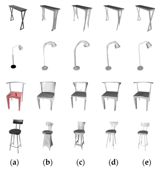
Figure 7.
Quantitative Analysis of Components. (a) Input image; (b) without prune; (c) without refinement; (d) full model; (e) ground truth.
We further analyzed the time consumption of the designed components. Table 3 shows that the time required for pruning is 32.1 ms, and the time required for refining is 34.0 ms. The time required for the full model to perform an inference is 51.9 ms, and the inference speed of the model is acceptable.
Table 3.
Time complexity analysis.
4.4. Comparison of Different Network Layers
We compare the performance of the local refinement module under different network layers. Table 4 shows the CD value and F-score value of local patch refinement under MLP, GCN, and FAGCN. As can be seen from the table, the structure using FAGCN performs the best, followed by GCN, and the worst using MLP.
Table 4.
Comparison of different network layers.
The worst performance of the network using the MLP layer is due to the fact that the MLP does not use the structural information of the mesh, ignores the connection between mesh points, and is not good at recovering mesh details. The effect of GCN is slightly better, but since GCN is only equivalent to a low-pass filter, although it can effectively filter out high-frequency noise, it cannot effectively utilize the high-frequency detail features of the mesh. On the other hand, FAGCN can learn the filters of different frequency bands from the data to adaptively utilize different frequency features, so it performs best.
4.5. Comparison between Basic Patch and Extended Patch
In this section, we explore the distinctions between a basic patch and an extended patch. Figure 8 compares the visualization outcomes of utilizing two distinct network patches. It can be seen that the visual effect of using the extended patch is better, while the reconstruction result using the basic patch is very unnatural at the connection between the patch and the mesh. This shows that the extended patch retains the one-way edge from the mesh to the patch so that the network can learn useful information at the connection. At the same time, a regularization term can also be applied to the connection to prevent abnormal points and self-intersections in the stitched mesh, making the connection smoother and more natural.
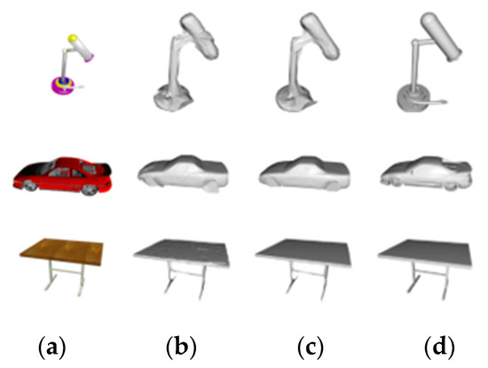
Figure 8.
Comparison between basic patch and extended patch. (a) Input image; (b) with the basic patch, (c) with the extended patch, (d) Ground truth.
4.6. Comparison of Different Patches Size
In this section, we explore the effect of subgraph size on the performance of the proposed method. Figure 9 shows the CD values of the network for various subgraph sizes. When K = 5, the CD value is the smallest, at 1.763. When K is less than 5, the patch gradually shrinks as K decreases. As a result of the neural network’s inability to obtain sufficient local data, the CD value exhibits a sharp upward trend, and the network’s performance begins to deteriorate. However, when K is greater than 5, the CD value begins to exhibit a slight upward trend as the patch size increases. This is because the patch is too large and the network is affected by distant, irrelevant points, which degrades network performance.
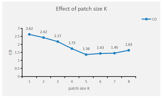
Figure 9.
Effect of patch size K on network performance.
4.7. Comparative Experiments on the Pix3D Dataset
In this section, we evaluate the generalization performance of the proposed model on real-world datasets. Specifically, we use the model trained on ShapeNet [1] to test the Pix3D [2] dataset. Since the background of the real dataset will interfere with the effect of reconstruction, we adopt the same method as TMNET [18], which uses a mask to manually separate the reconstructed objects and uses padding and resize operations to resize the image to a size of 224 × 224. Figure 10 shows the reconstruction results of our method, AtlasNet reconstruction, and TMNET on the Pix3D dataset. Compared to AtlasNet and TMNET, our method still handles objects with complex topologies well and is balanced in high and low curvature regions. This shows that our method can be well extended to real images.
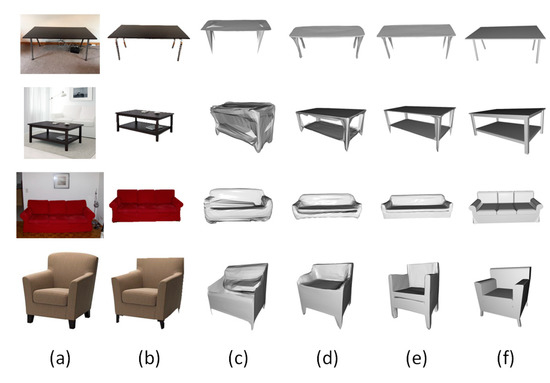
Figure 10.
Qualitative results on Pix3D dataset. (a) RGB image, (b) image without background, (c) Atlasnet, (d) TMNET, (e) Ours, (f) Ground truth.
Our method can recover correct holes in real-world datasets because the pruning strategy after introducing hole constraints can to some extent eliminate the limitations of data-driven error estimation networks. This makes our method perform better than TMNET on the untrained dataset.
5. Conclusions
In this paper, we propose a network framework for mesh reconstruction from a single image. The framework utilizes a global-to-local structure that combines MLP and GNN. Simultaneously, we propose a new grid pruning strategy under the 2D hole constraint, which overcomes the limitation of the 0-genus template. Then, the network is transitioned from global to local by an extended patch extraction module, and the high and low frequency local meshes are fine-tuned using a two-branch frequency adaptive local refinement structure to obtain a smooth mesh with rich mesh details. The method achieves the best quantitative results with a CD of 1.763 and an F-score of 85.40 on the ShapeNet dataset. Compared with other methods, our method can deal with holes with small areas and infrequent locations. Additionally, our method accurately restores details in high-curvature parts while maintaining the smoothness of low-curvature parts. However, it is difficult for our model to reconstruct objects with occlusions. Occluded images have semantic ambiguity, making it difficult for existing methods to reconstruct the occluded parts. In the future, we will explore the introduction of symmetry priors to improve the performance of 3D reconstruction networks.
Author Contributions
Conceptualization, methodology, writing—original draft, F.W.; supervision, funding acquisition, writing—review and editing, Q.L. All authors have read and agreed to the published version of the manuscript.
Funding
This study is jointly supported by the National Natural Science Foundation of China (61871138) and the Natural Science Foundation of Guangxi Province (2017GXNSFAA198371).
Institutional Review Board Statement
Not applicable.
Informed Consent Statement
Informed consent was obtained from all subjects involved in the study.
Data Availability Statement
Not applicable.
Acknowledgments
The authors are grateful to the ShapeNet team for providing the dataset. We also wish to thank the anonymous referees who reviewed this paper for their comments and recommendations.
Conflicts of Interest
The authors declare no conflict of interest.
References
- Chang, A.X.; Funkhouser, T.; Guibas, L.; Hanrahan, P.; Huang, Q.; Li, Z.; Savarese, S.; Savva, M.; Song, S.; Su, H.; et al. An information-rich 3d model repository. arXiv 2015, arXiv:1512.03012. [Google Scholar] [CrossRef]
- Sun, X.; Wu, J.; Zhang, X.; Zhang, Z.; Zhang, C.; Xue, T.; Tenenbaum, J.B.; Freeman, W.T. Pix3d: Dataset and methods for single-image 3d shape modeling. In Proceedings of the IEEE Conference on Computer Vision and Pattern Recognition, Salt Lake City, UT, USA, 18–22 June 2018; pp. 2974–2983. [Google Scholar] [CrossRef]
- Xiang, Y.; Mottaghi, R.; Savarese, S. Beyond pascal: A benchmark for 3d object detection in the wild. In Proceedings of the IEEE Winter Conference on Applications of Computer Vision, Steamboat Springs, CO, USA, 24–26 March 2014; pp. 75–82. [Google Scholar] [CrossRef]
- Chen, Z.; Zhang, H. Learning implicit fields for generative shape modeling. In Proceedings of the IEEE/CVF Conference on Computer Vision and Pattern Recognition, Long Beach, CA, USA, 16–17 June 2019; pp. 5939–5948. [Google Scholar] [CrossRef]
- Mescheder, L.; Oechsle, M.; Niemeyer, M.; Nowozin, S.; Geiger, A. Occupancy networks: Learning 3d reconstruction in function space. In Proceedings of the IEEE/CVF Conference on Computer Vision and Pattern Recognition, Long Beach, CA, USA, 16–17 June 2019; pp. 4460–4470. [Google Scholar] [CrossRef]
- Xu, Q.; Wang, W.; Ceylan, D.; Mech, R.; Neumann, U. Disn: Deep implicit surface network for high-quality single-view 3d reconstruction. In Proceedings of the 33rd International Conference on Neural Information Processing Systems, Vancouver, BC, Canada, 8–12 December 2019; pp. 492–502. [Google Scholar]
- Chen, Z.; Tagliasacchi, A.; Zhang, H. Bsp-net: Generating compact meshes via binary space partitioning. In Proceedings of the IEEE/CVF Conference on Computer Vision and Pattern Recognition, Seattle, WA, USA, 13–19 June 2020; pp. 45–54. [Google Scholar] [CrossRef]
- Choy, C.B.; Xu, D.; Gwak, J.; Chen, K.; Savarese, S. 3d-r2n2: A unified approach for single and multi-view 3d object reconstruction. In Proceedings of the European Conference on Computer Vision, Amsterdam, The Netherlands, 11–14 October 2016; pp. 628–644. [Google Scholar] [CrossRef]
- Tatarchenko, M.; Dosovitskiy, A.; Brox, T. Octree generating networks: Efficient convolutional architectures for high-resolution 3d outputs. In Proceedings of the IEEE International Conference on Computer Vision, Venice, Italy, 22–29 October 2017; pp. 2088–2096. [Google Scholar] [CrossRef]
- Tulsiani, S.; Zhou, T.; Efros, A.A.; Malik, J. Multi-view supervision for single-view reconstruction via differentiable ray consistency. In Proceedings of the IEEE Conference on Computer Vision and Pattern Recognition, Honolulu, HI, USA, 21–26 July 2017; pp. 2626–2634. [Google Scholar] [CrossRef]
- Wu, J.; Zhang, C.; Zhang, X.; Zhang, Z.; Freeman, W.T.; Tenenbaum, J.B. Learning shape priors for single-view 3d completion and reconstruction. In Proceedings of the European Conference on Computer Vision (ECCV), Munich, Germany, 8–14 September 2018; pp. 646–662. [Google Scholar] [CrossRef]
- Fan, H.; Su, H.; Guibas, L. A point set generation network for 3d object reconstruction from a single image. In Proceedings of the IEEE Conference on Computer Vision and Pattern Recognition, Honolulu, HI, USA, 21–26 July 2017; pp. 605–613. [Google Scholar] [CrossRef]
- Jiang, L.; Shi, S.; Qi, X.; Jia, J. Gal: Geometric adversarial loss for single-view 3d-object reconstruction. In Proceedings of the European Conference on Computer Vision (ECCV), Munich, Germany, 8–14 September 2018; pp. 802–816. [Google Scholar] [CrossRef]
- Zhao, M.; Xiong, G.; Zhou, M.; Shen, Z.; Wang, F.-Y. 3D-RVP: A method for 3D object reconstruction from a single depth view using voxel and point. Neurocomputing 2020, 430, 94–103. [Google Scholar] [CrossRef]
- Jack, D.; Pontes, J.K.; Sridharan, S.; Fookes, C.; Shirazi, S.; Maire, F.; Eriksson, A. Learning free-form deformations for 3d object reconstruction. In Proceedings of the Asian Conference on Computer Vision, Perth, Australia, 2–6 December 2018; pp. 317–333. [Google Scholar] [CrossRef]
- Wang, N.; Zhang, Y.; Li, Z.; Fu, Y.; Liu, W.; Jiang, Y.-G. Pixel2mesh: Generating 3d mesh models from single rgb images. In Proceedings of the European Conference on Computer Vision (ECCV), Munich, Germany, 8–14 September 2018; pp. 52–67. [Google Scholar] [CrossRef]
- Kanazawa, A.; Tulsiani, S.; Efros, A.A.; Malik, J. Learning category-specific mesh reconstruction from image collections. In Proceedings of the European Conference on Computer Vision (ECCV), Munich, Germany, 8–14 September 2018; pp. 371–386. [Google Scholar] [CrossRef]
- Pan, J.; Han, X.; Chen, W.; Tang, J.; Jia, K. Deep mesh reconstruction from single rgb images via topology modification networks. In Proceedings of the IEEE/CVF International Conference on Computer Vision, Seoul, Republic of Korea, 27 October–2 November 2019; pp. 9964–9973. [Google Scholar] [CrossRef]
- Smith, E.J.; Fujimoto, S.; Romero, A.; Meger, D. Geometrics: Exploiting geometric structure for graph-encoded objects. arXiv 2019, arXiv:1901.11461. [Google Scholar] [CrossRef]
- Tang, J.; Han, X.; Pan, J.; Jia, K.; Tong, X. A skeleton-bridged deep learning approach for generating meshes of complex topologies from single rgb images. In Proceedings of the IEEE/CVF Conference on Computer Vision and Pattern Recognition, Long Beach, CA, USA, 16–17 June 2019; pp. 4541–4550. [Google Scholar] [CrossRef]
- Shi, Y.; Ni, B.; Liu, J.; Rong, D.; Qian, Y.; Zhang, W. Geometric Granularity Aware Pixel-To-Mesh. In Proceedings of the IEEE/CVF International Conference on Computer Vision, Montreal, BC, Canada, 11–17 October 2021; pp. 13097–13106. [Google Scholar] [CrossRef]
- Yuan, Y.; Tang, J.; Zou, Z. Vanet: A view attention guided network for 3d reconstruction from single and multi-view images. In Proceedings of the 2021 IEEE International Conference on Multimedia and Expo (ICME), Shenzhen, China, 5–9 July 2021; pp. 1–6. [Google Scholar] [CrossRef]
- Zheng, X.; Jiang, B.; Zhang, J. Deformation representation based convolutional mesh autoencoder for 3D hand generation. Neurocomputing 2021, 444, 356–365. [Google Scholar] [CrossRef]
- Lorensen, W.E.; Cline, H.E. Marching cubes: A high resolution 3D surface construction algorithm. ACM SIGGRAPH Comput. Graph. 1987, 21, 163–169. [Google Scholar] [CrossRef]
- Armstrong, M.A. Basic Topology; Springer Science & Business Media: New York, NY, USA, 2013. [Google Scholar]
- Li, Q.; Han, Z.; Wu, X. Deeper insights into graph convolutional networks for semi-supervised learning. In Proceedings of the Thirty-Second AAAI Conference on Artificial Intelligence, New Orleans, LA, USA, 2–7 February 2018; pp. 3538–3545. [Google Scholar]
- Bo, D.; Wang, X.; Shi, C.; Shen, H. Beyond low-frequency information in graph convolutional networks. In Proceedings of the AAAI Conference on Artificial Intelligence, Hong Kong, China, 2–9 February 2021; pp. 3950–3957. [Google Scholar]
- Xie, H.; Yao, H.; Zhou, S.; Zhang, S.; Tong, X.; Sun, W. Toward 3d object reconstruction from stereo images. Neurocomputing 2021, 463, 444–453. [Google Scholar] [CrossRef]
- Wen, C.; Zhang, Y.; Li, Z.; Fu, Y. Pixel2mesh++: Multi-view 3d mesh generation via deformation. In Proceedings of the IEEE/CVF International Conference on Computer Vision, Seoul, Republic of Korea, 27 October–2 November 2019; pp. 1042–1051. [Google Scholar] [CrossRef]
- Hartley, R.; Zisserman, A. Multiple View Geometry in Computer Vision; Cambridge University Press: Cambridge, UK, 2003. [Google Scholar]
- Furukawa, Y.; Ponce, J. Accurate, Dense, and Robust Multiview Stereopsis. IEEE Trans. Pattern Anal. Mach. Intell. 2009, 32, 1362–1376. [Google Scholar] [CrossRef] [PubMed]
- Peng, B.; Wang, W.; Dong, J.; Tan, T. Learning pose-invariant 3D object reconstruction from single-view images. Neurocomputing 2020, 423, 407–418. [Google Scholar] [CrossRef]
- He, K.; Zhang, X.; Ren, S.; Sun, J. Deep residual learning for image recognition. In Proceedings of the IEEE Conference on Computer Vision and Pattern Recognition, Las Vegas, NV, USA, 27–30 June 2016; pp. 770–778. [Google Scholar] [CrossRef]
- Gkioxari, G.; Johnson, J.; Malik, J. Mesh r-cnn. In Proceedings of the IEEE/CVF International Conference on Computer Vision, Seoul, Republic of Korea, 27 October–2 November 2019; pp. 9785–9795. [Google Scholar] [CrossRef]
- Kipf, T.N.; Welling, M. Semi-supervised classification with graph convolutional networks. arXiv 2016, arXiv:1609.02907. [Google Scholar] [CrossRef]
- Veličković, P.; Cucurull, G.; Casanova, A.; Romero, A.; Lio, P.; Bengio, Y. Graph attention networks. arXiv 2017, arXiv:1710.10903. [Google Scholar] [CrossRef]
- Groueix, T.; Fisher, M.; Kim, V.G.; Russell, B.C.; Aubry, M. A papier-mâché approach to learning 3d surface generation. In Proceedings of the IEEE Conference on Computer Vision and Pattern Recognition, Salt Lake City, UT, USA, 18–22 June 2018; pp. 216–224. [Google Scholar] [CrossRef]
- Suzuki, S. Topological structural analysis of digitized binary images by border following. Comput. Vis. Graph. Image Process. 1985, 30, 32–46. [Google Scholar] [CrossRef]
- Loop, C. Smooth Subdivision Surfaces Based on Triangles. Master’s Thesis, University of Utah, Salt Lake City, UT, USA, 1987. [Google Scholar]
- Kato, H.; Ushiku, Y.; Harada, T. Neural 3d mesh renderer. In Proceedings of the IEEE Conference on Computer Vision and Pattern Recognition, Salt Lake City, UT, USA, 18–22 June 2018; pp. 3907–3916. [Google Scholar] [CrossRef]
- Kingma, D.P.; Ba, J. Adam: A method for stochastic optimization. arXiv 2014, arXiv:1412.6980. [Google Scholar] [CrossRef]
- Knapitsch, A.; Park, J.; Zhou, Q.; Koltun, V. Tanks and Temples: Benchmarking Large-Scale Scene Reconstruction. ACM Trans. Graph. 2017, 36, 78. [Google Scholar] [CrossRef]
- Chiang, W.-L.; Liu, X.; Si, S.; Li, Y.; Bengio, S.; Hsieh, C.-J. Cluster-gcn: An efficient algorithm for training deep and large graph convolutional networks. In Proceedings of the 25th ACM SIGKDD International Conference on Knowledge Discovery & Data Mining, Anchorage, AK, USA, 4–8 August 2019; pp. 257–266. [Google Scholar] [CrossRef]


Disclaimer/Publisher’s Note: The statements, opinions and data contained in all publications are solely those of the individual author(s) and contributor(s) and not of MDPI and/or the editor(s). MDPI and/or the editor(s) disclaim responsibility for any injury to people or property resulting from any ideas, methods, instructions or products referred to in the content. |
© 2023 by the authors. Licensee MDPI, Basel, Switzerland. This article is an open access article distributed under the terms and conditions of the Creative Commons Attribution (CC BY) license (https://creativecommons.org/licenses/by/4.0/).