A System for the Automatic Detection and Evaluation of the Runway Surface Cracks Obtained by Unmanned Aerial Vehicle Imagery Using Deep Convolutional Neural Networks

Abstract

The timely detection and recognizing of distress on an airport pavement is crucial for safe air traffic. For this purpose, a physical inspection of the airport maneuvering areas is regularly carried out, which might be time-consuming due to its size. One of the modern approaches to speeding up this process is unmanned aerial vehicle imagery followed by an automatic evaluation. This study explores the automatic detection of the transverse crack, its dimension measurement, and position determination within the slab on the concrete runway. The aerial image data were obtained from flights at the given altitude above the runway and processed using commercial multi-view reconstruction software to create a dataset for the training, verification, and testing of a YOLOv2 object detector. Once the crack was detected, the main features were obtained by image segmentation and morphological operations. The YOLOv2 detector was tuned with 3279 images until the detection metrics (average precision AP = 0.89) reached sufficient value for real deployment. The detected cracks were further processed to determine their position within the concrete slab, and their dimensions, i.e., length and width, were measured. The automated crack detection and evaluation system developed in this study was successfully verified on the experimental section of the runway as an example of practical application. It was proven that unmanned aerial vehicle imagery is efficient over broad areas and produces impressive results with the combination of artificial intelligence.

1. Introduction

The surface of airport pavements must be kept in high-grade condition to ensure the movements of the aircraft are safe during take-off, landing, and taxiing. Aviation regulations require that the surface of the paved airport must be regularly monitored and evaluated for the occurrence of distress. This process, often called pavement stocktaking, is usually manually performed by visual inspection to identify and assess the signs of individual types of distress every year. Due to the size of the airport and the air traffic volume, this procedure often requires the airport authority to restrict air traffic, which makes the process time-consuming. The data collected during the inspection helps the airport authority to plan necessary maintenance and repairs. One efficient way to reduce the time and effort involved in the human inspection process is Unmanned Aerial Vehicle (UAV) imagery followed by a deep learning algorithm for object detection. Through aerial photography, an overview of a large area is obtained, and another point of view is obtained. The image quality and visible details then depend on the camera and flight altitude [1]. As a part of artificial intelligence, the deep learning framework creates a detector to recognize, locate, and label the desired distress, and computer vision methods such as image segmentation and morphological operations are often used for further distress analysis.

The approach based on deep learning using convolutional neural networks has become practical for object detection due to its speed and accuracy. Object detection aims to replicate the ability of humans to recognize and identify objects in video or images by using a computer. Regions with Convolutional Neural Network (R-CNN) [2] is a two-stage detection algorithm that combines rectangular region proposals with convolutional neural network features. The first stage looks for a subset of regions that may contain an image object, while the second classifies the objects in each region. A Fast Region-based Convolutional Neural Network (Fast R-CNN) [3] improves training and testing speed while increasing detection accuracy, since the computations for overlapping regions are shared. The Fast R-CNN detector processes the entire image, unlike the R-CNN method, which only crops and resizes region proposals. A Faster Region-based Convolutional Neural Network (Faster R-CNN) [4] adds a Region Proposal Network (RPN) that shares full-image convolutional features with the detection network, thus enabling nearly cost-free region proposals. The RPN takes advantage of anchor boxes and generates region proposals faster and more accurately. A Single Shot Multibox Detector (SSD) [5] is a single-stage object detection method that applies a discretization algorithm to create a set of default boxes for detecting objects. The network then generates scores and adjusts the boxes based on the predicted object categories. The network also combines predictions from multiple feature maps to efficiently handle different sizes of objects. The SSD is considered faster than two-stage detectors, such as the Faster R-CNN detector. You Only Look Once (YOLO) is a single-stage object detector that excels in high speed and accuracy. YOLO was first published by Redmon et al. [6] in 2015 and has become one of the most popular detectors, even for pavement distress detection. The basic principle included a single neural network directly predicting bounding boxes and class probabilities from full images in one evaluation. Since then, the YOLO family has grown to include more variants as its performance has gradually increased. Redmond and Farhadi introduced YOLO9000 and YOLOv2 in 2016, and subsequently, they announced an enhancement called YOLOv3 in 2018. Bochkovskiy et al. launched YOLOv4 in 2020. Jocher refined YOLOv4 and released YOLOv5 in the middle of 2020. Li et al. created the YOLOv6 series for industry-level applications in 2022. In the same year, Wang et al. (the same research team that introduced YOLOv4) developed YOLOv7 [7,8,9,10,11,12].

Many studies dealing with automatic distress detection and evaluation have recently been published. These studies primarily focus on road distress with asphalt or concrete cover, defects on bridge structures or dams, disruption in building walls, and to a minor extent, distress on airport pavements. In most cases, they target cracks as the basic type of distress. Similarly, the methods of image acquisition vary, from using a smartphone, a digital camera, a digital camera mounted on a moving vehicle, aerial (UAV) imagery, multi- or hyperspectral imaging to laser scanning, or the application of the light detection and ranging (LiDAR) method.

Absolon et al. [13] proposed inspecting the runway and other movement areas using the UAV during airport operations instead of a controller driving a car and looking for dangerous objects. The advantages of the UAV over the conventional method are its flexibility and reduced time. The control processes are faster and can be executed more often. In addition, the data backup and evaluation of small surface cracks are also beneficial.

Mogawer et al. [14] conducted a study evaluating the applicability of UAVs for roadway pavement condition analysis. The core image dataset was collected during the flights of UAVs at Fitchburg Municipal Airport, USA, and was analyzed using two deep learning methods (SSD Mobilenet_V1 network, U-Net) and CrackIT toolbox. The deep learning methods outperformed CrackIT and generated satisfactory crack detection results. While the SSD Mobilenet_V1 network highlighted the detected cracks with rectangular boxes, U-Net could spot cracks at the pixel level, which is necessary for pavement condition index (PCI) values calculation. CrackIT is a toolbox created in the Matlab environment, which detects road pavement surface cracks distresses and characterizes them into types based on image processing and pattern recognition. Although the CrackIT tool can provide good characterization and detection results, dealing with fragile cracks, which are less than 2 mm wide, can be challenging. This is due to the difficulty in distinguishing them from raveling distresses. However, CrackIT aims to detect cracks at least 2 mm in width, in line with the guidelines provided by road experts [15].

Mandal et al. [16] gathered 9053 road images taken from a vehicle-mounted smartphone, which were split into 7240 for training and 1813 as testing samples. The types of cracks found in the road images were categorized into linear cracks (longitudinal, lateral), alligator cracks, and other corruptions. The YOLOv2 detector was used for automatic crack detection and transfer learning with ResNet-101 to speed up the training process. It was investigated that other deep learning frameworks, such as YOLOv3, SSD, or Faster R-CNN, failed to achieve the same score rate as YOLOv2 in the same samples.

Majidifard et al. [17] compiled a dataset consisting of road images captured from two camera views of an identical pavement segment, i.e., wide-view and top-down-view angles, each of 7237 images. The wide-view angles were used to classify distresses, while top-down-view images were used for calculating their density. The images consisted of distress types critical for pavement condition assessment, such as reflective, transverse, block, longitudinal, alligator, sealed transverse, sealed longitudinal, and longitudinal lane cracking, along with potholes. The dataset was evaluated using the YOLOv2 and Faster R-CNN boosted by transfer learning, where YOLOv2 resulted in more accurate distress characterization than the Faster R-CNN model.

Hu et al. [18] compared the YOLOv5 model of versions YOLOv5s, YOLOv5m, YOLOv5l, and YOLOv5x for road crack detection based on 3001 images taken by a digital camera depending on the detection rate and detection efficiency. The individual variants of YOLOv5 were evaluated on 640 × 640 images, where YOLOv5s had the best trade-off between speed and accuracy.

Furthermore, other applications for crack detection and description have been developed. For instance, a unique algorithm called MorphLink-C was developed to analyze images of concrete structures captured by UAVs. It visually analyzes the high-resolution data and finds the pixels of the separated and grouped cracks. The number of pixels was used to calculate the crack width, which was then converted into millimeters. The difference between the computed width and the actual survey was from 3% to 50%, which met the limit survey error range, which was set to 0.1 mm [19]. I-Crack is a tool that detects and measures the length and width of reinforced concrete cracks in high-resolution panoramic images. It was built on algorithms that are commonly used in Matlab. The program consists of four main building blocks: (1) an algorithm for detecting edges, (2) morphological operations for filling cracks, (3) the separation of cracks from surface defects, and (4) the measurement of the crack width. I-Crack was evaluated using crack patterns and widths manually collected from the tests of nine walls to ensure that the algorithm correctly detected cracks, followed by comparing the predicted width. The maximal difference between the I-Crack and the manual measurements was 0.48 mm, which was considered insignificant [20].

The movement area of an airport is defined as a part of an aerodrome to be used for the take-off, landing, and taxiing of aircraft, consisting of a maneuvering area and apron(s). The maneuvering area is part of an aerodrome for take-off, landing, and taxiing aircraft, excluding aprons. A runway is a defined rectangular area on a land aerodrome prepared for landing and aircraft take-off [21]. The runway is considered a critical element of maneuvering areas, the surface of which is usually built of concrete or asphalt at civil and military airports. One of the most common types of airport pavement distress is a crack, from which other types of distress can be further derived according to their orientation, location, and length within a slab in the concrete surface. The width of a crack is considered the most crucial factor that affects air traffic safety. Depending on the severity, the crack can be categorized into three levels: small (the average crack width is less than or equal to 0.2 cm), medium (the average crack width is greater than 0.2 cm and less than 1.0 cm), or large (the average crack width is greater than or equal to 1.0 cm). According to North Atlantic Treaty Organization (NATO) terminology in determining airfield pavement conditions through visual surveys, longitudinal, transverse, and diagonal cracks correspond to distress code 63 [22].

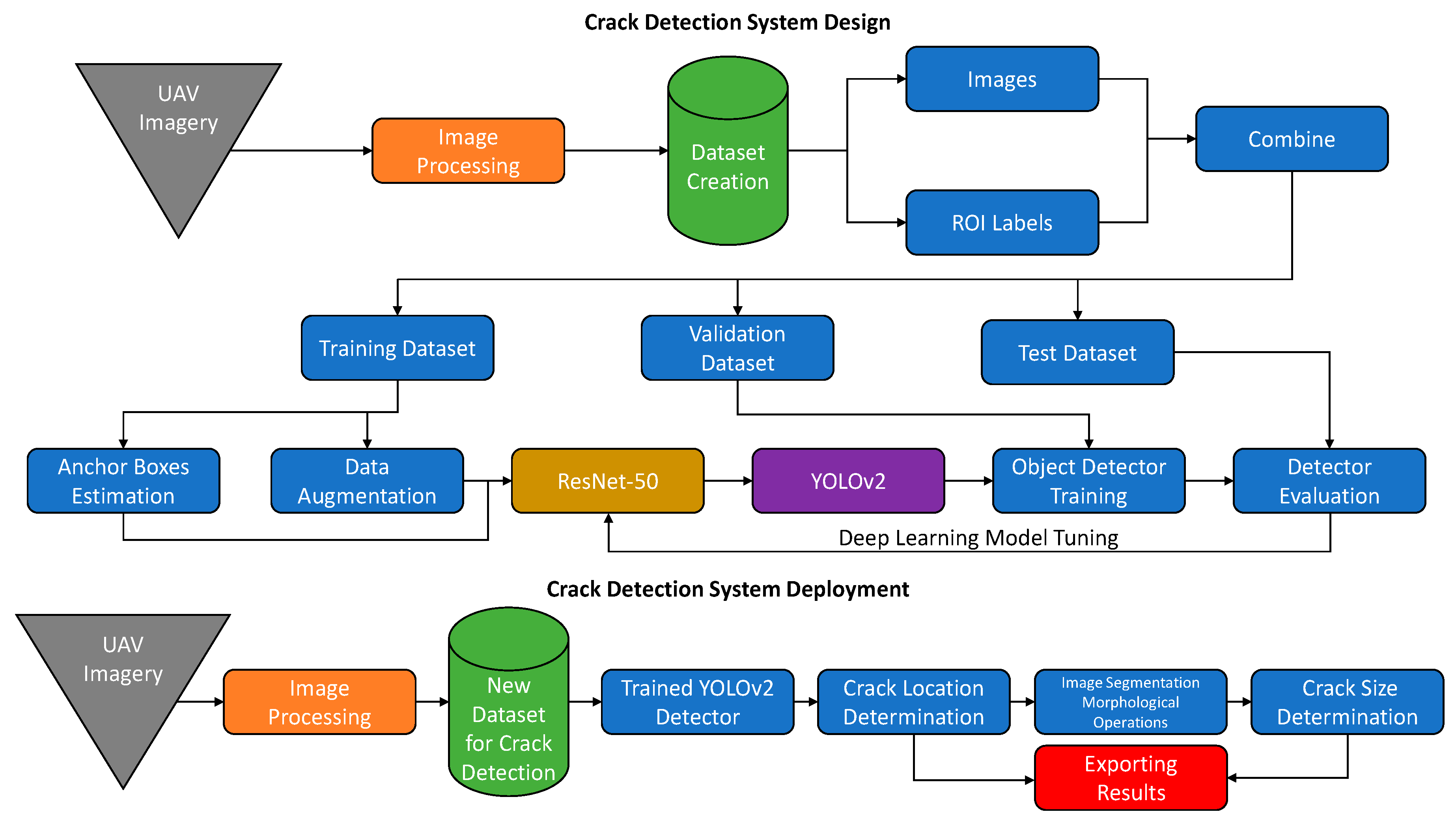
The main goal of this article is to present an automated system for the automatic detection and evaluation of distress on a concrete runway through artificial intelligence using aerial imagery. The system includes runway image acquisition through UAV, captured image data processing for dataset creation, crack labeling, deep learning model design based on the YOLOv2 object detector, its training, and performance evaluation. The system was tuned until the required accuracy was reached and was sequentially deployed into live operation. Once the crack was detected, its position and size were computed by counting individual pixels in a binary image (Figure 1). The transverse crack was selected as the main component to verify the functionality of the system.

Although newer versions of the YOLO detector have introduced many improvements in accuracy and functionality, the popular YOLOv2 was chosen for this project. YOLOv2 is generally faster than later versions due to its simpler architecture and fewer layers, which allows it to process images more quickly. The simple architecture is also beneficial for easier network customization for a specific use case. While later versions of YOLO have improved the accuracy, the differences are not significant enough to justify the additional computational cost. YOLOv2 has a smaller model size than the newer versions, which is beneficial for limited computational resources or low-power devices and requires less memory to run in a smooth way. Compared with YOLOv5, it can perform better on small objects by using the anchor boxes, which improves the detection of small-scale entities, while YOLOv5 uses anchor-free object detection, which may lead to worse detection of small targets. On the other hand, YOLOv5 anchor-free detection provides more accurate object detection results and reduces the need for hyperparameter tuning, which makes the algorithm easier to use. YOLOv5 has advanced architecture and adds other features to improve accuracy, but it has not yet been fully implemented in the Matlab environment.

2. Materials and Methods

2.1. Study Site Subject

The former military airport Bechyne located in southern Bohemia in the Czech Republic was selected as a source for collecting the image data for the distress database. The runway has a concrete surface with dimensions 2400 m in length and 60 m in width. The facility was officially closed for air traffic, including air traffic service, in 1993, and the regular maintenance of movement areas was halted. Due to the terminated maintenance, there has been a gradual development of distresses, and the airport could serve as a feed for the generation of the image database, unlike operational airports where a continuous maintenance system is established and the occurrence of distresses is minimal. For the UAV flights, airspace was requested through the military branch of the Airspace Management Cell (AMC) of the Czech Republic and published via Notice to Airman (NOTAM). The temporarily reserved part of the airspace comprised a block with a rectangular base of 2400 m in length and 450 m in width, including a runway with a taxiway system and unpaved areas vertically extending to 91 m (300 ft) Above Ground Level (AGL).

2.2. Equipement and Procedure

A consumer quadcopter used in this project, a DJI Mavic 2 Enterprise Dual, was approved for military use by the Military Aviation Authority (MAA) of the Czech Republic. It features a fully stabilized 3-axis gimbal camera with a Forward Looking Infrared (FLIR) longwave thermal camera and a visual camera that simultaneously provides both infrared and visible light imaging. The visual camera has a 1/2.3″3″ CMOS sensor and provides the maximum image size of 4056 × 3040 (4:3) or 4056 × 2280 (16:9) pixels, a field of view of 85°, with an aperture of f/2.8 at infinity. The thermal camera has an uncooled Vox microbolometer sensor, which provides the maximal image size of 640 × 480 (4:3) or 640 × 360 pixels (16:9), a field of view of 57°, with an aperture of f/1.1 at infinity [23]. The model was supplied with four intelligent flight batteries covering a flight time of approximately 20 min.

The DJI Pilot application (Shenzhen, China), version v2.5.1.10, installed in the flight controller, was used for flight planning. After visual inspection, the runway was divided into four sections; thus, the region of interest had a rectangular shape. Three were intended as a source for creating the crack database, and the fourth was for testing and experimental purposes. The following flight parameters were set for mapping in the application. The width of the section corresponded to the width of the runway and the length of the expected flight time with one battery. The flight altitude was set to 25 m (82 ft) AGL, with the forward overlap at 80% and the side overlap at 70%. The flight trajectory was chosen to be parallel to the runway axis. This solution reduces the number of pivot points where the UAV changes the flight direction resulting in reduced speed and increased imaging time. The length of the mapped section could be extended this way, and the battery capacity could be better utilized.

The captured overlapping images were stitched together using the commercial photogrammetric software Agisoft Metashpe Professional Edition (St. Petersburg, Russia) [24], Node-Locked Educational License, version v1.5.2.7838, to generate an orthomosaic map of each section of the runway. The first section of the runway consisted of 383 images, the second consisted of 391 images, the third consisted of 393 images, and the fourth (test and experimental) section consisted of 394 images. The images were processed with the following workflow steps. The image alignment to build a sparse point cloud: accuracy was set to low, generic preselection was enabled, the key point limit was set to 40,000, the tie point limit was set to 4000, and the adaptive camera model fitting was enabled. The dense point cloud building: quality was set to low, depth filtering was set to mild, and calculate point color was enabled. The source data for mesh building was a dense cloud, the surface type height field with low depth maps quality. The digital elevation model was built using a dense point cloud with enabled interpolation. The low processing parameters were set due to faster image processing. The orthomosaic was built using mosaic blending mode; as a surface was used, a digital elevation model and hole filling were enabled [1]. The Ground Sample Distance (GSD) of the first section of the runway was calculated to be 8.52 mm/pix, the second section to be 8.58 mm/pix, the third to be 7.02 mm/pix, and the last, the test section, to be 6.41 mm/pix. The different altitudes of the individual runway sections caused the difference in GSD values.

Data plotting, calculations, and YOLOv2 detector training were computed in the programming language and numeric computing environment Matlab, using a computer with the operating system Windows 11, an Intel Core i9-9980HK CPU @ 2.40 GHz, 32 GB RAM, and an NVIDIA^® GeForce^® RTX 2060 graphic card.

2.3. Image Data Preparation and Labeling

The runway orthomosaic, the first to the third section, obtained by Agisoft Metashape was split into 224 × 224 image blocks. Each block was evaluated as positive, containing a crack, or negative, with no crack. The positive blocks containing longitudinal cracks were rotated by 90 degrees and horizontally and vertically flipped to expand the image database. The resulting dataset consisted of 3279 images, each containing one or more transverse cracks. The images were loaded into the Matlab Image Labeler App, where the transverse cracks, such as the Region of Interest (ROI), were manually labeled with a rectangular shape.

The labeled data were exported as a ground truth object for the YOLOv2 object detector training.

2.4. Deep Learning Model Design

A deep convolutional neural network based on the YOLOv2 framework was created in the Matlab Deep Learning Toolbox for automatic transverse crack detection. The network comprises a pair of subnetworks, a feature extraction network followed by a detection network. A pretrained convolutional neural network, ResNet-50, was used as a feature extractor, and transfer learning was applied to speed up the training process. The main advantage of transfer learning is skipping the time-consuming training steps where the learnable parameters (weights and biases) obtained from training the model over a large dataset are only fine-tuned to accommodate the network to classify a different target dataset.

ResNet-50 is a variation of the residual network trained on more than one million images from the ImageNet database consisting of building (residual) blocks of convolutional layers with residual connections known as skip or shortcut connections. Through these connections, the input can skip the main branch of convolutional layers, providing a more straightforward path within the network, which helps to minimize the issue of vanishing gradients during the early stages of training. The residual blocks are then grouped into a stack and can be formally described:

$$y_l\left(x, W\right)=f(h\left(x\right)+F\left(x, W\right))$$

(1)

where x is the input of the block, h is the shortcut function, F is the mapping carried out by a block of one or more consecutive convolutional layers, W is the weights of these convolutional layers, f is a Rectified Linear Unit (ReLU), and y is the mapping describing the residual block l as a function of the input x and the weights W [25].

The ResNet-50 architecture consists of an initial residual block followed by the basic residual blocks, also called bottleneck blocks, applied along the network. The initial block starts with the input layer of the image size of 224 × 224 × 3, followed by the convolutional layer. Convolution is a mathematical operation usually implemented as the cross-correlation function [26] and can be described as function S with filter (also called kernel) K over the two-dimensional image I:

$$S\left(i, j\right)=\left(I \times K\right)\left(i, j\right)={\displaystyle \sum }_m{\displaystyle \sum }_{n}I\left(i+m, j+n\right) K(m, n)$$

(2)

In machine learning terminology, the function S is referred to as a feature map. The first convolutional layer uses 64 filters of 7 × 7 pixels with a stride of 2, and thus produces 64 feature maps with half the lateral size of the input image.

The features are then regularized through a batch normalization layer that performs the standardization of the input corresponding to the subtraction of the mean of the batch and the division by the standard deviation. A batch normalization layer independently normalizes a mini-batch of data for each channel across all observations, and the convolutional neural network is trained faster.

The convolutional and batch normalization layers continue with a non-linearity by applying an activation function. The activation function is designed to resemble the behavior of real neurons and performs a non-linear transformation of the feature map, providing the input for the next convolutional layer. The widespread ReLU was used as an activation function. The ReLU function f returns the same value if the input x is positive and zero if the value is negative or null:

$$f\left(x\right)=\{\begin{array}{cc}x,& x > 0\\ 0,& x \le 0\end{array}=\mathit{max}(0, x)$$

(3)

The ReLU function rectifies the vanishing gradient problem and guarantees a high computation efficiency thanks to simple mathematical operations [27]. The initial residual block ends with a pooling layer, which reduces the spatial size of the convolved features and decreases the computational power to process the data. The ResNet-50 uses a max pooling layer returning the maximum value from the portion of an image covered by the 3 × 3 filter with a stride of 2.

The bottleneck blocks in the ResNet-50 architecture are composed of three convolutional layers with filters of size 1 × 1, 3 × 3, and 1 × 1, respectively. The convolutional layers with a stride of 2 perform the downsampling (conv3_1 and conv4_1), and batch normalization is carried out after each convolution before ReLU activation. The ResNet-50 has two variants of bottleneck blocks: the identity shortcut and the projection shortcut. The convolutional layers in the identity shortcut are connected to skip connection input; this block can be directly used when the input and output feature maps have the same dimension. The projection shortcut has an extra convolutional layer with a filter of size 1 × 1 present on the skip connection. When the dimensions change, there are two options: first, the shortcut still performs identity mapping, with extra zero entries padded for increasing the depth, or second, an extra 1 × 1 convolutional layer is used to match the dimensions. The deeper layers of the ResNet-50 feature extraction network (fifth stack, average pooling layer, fully connected layer, and softmax layer) were replaced with the YOLOv2 detection subnetwork. Thus, in this case, the ResNet-50 outputs feature maps that downsample the input image by a factor of 16 (224/16 = 14 × 14).

YOLOv2 is a state-of-the-art real-time object detection system providing a smooth trade-off between speed and accuracy in different scenarios [7]. It is a small convolutional network consisting of serially connected convolutions, ReLU, and batch normalization layers, followed by a transform layer and an output layer. The first two convolutional layers have filters of size 3 × 3 with a number of filters matching the number of channels in the ResNet-50 feature extraction layer output. The last convolution layer has a filter of size 1 × 1 with a number of filters depending on the number of anchor boxes, classes, and predictions per anchor box. The transform layer extracts activations of the last convolutional layer and transforms the bounding box predictions to fall within the bounds of the ground truth. The output layer provides the refined bounding box locations of the target objects. Figure 2 outlines the layers and operations of the ResNet-50 feature extraction network with the YOLOv2 detector. The upper part of the scheme depicts the feature maps obtained by different layers of the ResNet-50 and the final output of the YOLOv2 detector. The middle part schematically illustrates the representative layers of the network. The effect of the convolution, batch normalization, activation, and maximal pooling produced by the first layer of ResNet-50 from the input image is shown in the lower part of the scheme.

2.5. Estimating Anchor Boxes from Training Data

The YOLOv2 detector uses an idea called an anchor box to detect multiple objects with different shapes within the same image. Anchor boxes are a set of predefined bounding boxes of a certain height and width to capture the scale and aspect ratio of specific object classes to be detected and are typically chosen based on object sizes in the training dataset. For the efficient and precise performance of the detector, estimating the appropriate number of anchor boxes, including their shape and scale, is necessary. The k-means clustering algorithm, with a mean Intersection over Union (IoU) distance metric, was used to estimate the number of anchor boxes. The k-means clustering algorithm groups the similar ground truth boxes from the labeled training dataset. IoU measures the similarity between anchor boxes and ground truth boxes, and guarantees that it overlaps each other. The mean IoU distance metric d was calculated using the following formula:

$$d=1 - \mathit{IoU}$$

(4)

where IoU is the ratio between the intersection between anchor boxes and ground truth boxes to the area of union between anchor boxes and ground truth boxes.

Based on the clustering results analysis, the number of anchors was set to 20, corresponding to a mean IoU = 0.8424 as a trade-off between the number of anchors and the mean IoU (Figure 3). The clustered anchor boxes for transverse cracks are characterized in that the width is noticeably smaller than the height. The height then corresponds to the different lengths of the transverse crack.

2.6. YOLOv2 Object Detector Training

The YOLOv2 detection model dataset was split into 1967 images for training and 328 for validation. The input image is split throughout the training phase into an S × S grid, where each cell predicts B bounding boxes. A number of predicted bounding boxes is selected before the training phase, considering that each object has a different shape of anchor boxes [28]. For every bounding box, certain confidence is assigned. The confidence score represents the probability that an object is contained inside a bounding box and how accurate the decision is. In other words, it is the minimum score that the model will consider the prediction to be a true prediction. The output layer of the YOLOv2 network predicts refined bounding box locations by optimizing the mean squared error loss between predicted bounding boxes and the ground truth. The loss function consists of localization loss, confidence loss, and classification loss. The localization loss measures error between the predicted bounding box and the ground truth as follows:

$$K_1{\displaystyle \sum }_{i=0}^{s^2}{\displaystyle \sum }_{j=0}^B{1}_{ij}^{obj}\left[{\left(x_i-{\widehat{x}}_i\right)}^2+{\left(y_i-{\widehat{y}}_i\right)}^2\right]+K_2{\displaystyle \sum }_{i=0}^{s^2}{\displaystyle \sum }_{j=0}^B{1}_{ij}^{obj}\left[{\left(\sqrt{w_i}-\sqrt{{\widehat{w}}_i}\right)}^2+{\left(\sqrt{h_i}-\sqrt{{\widehat{h}}_i}\right)}^2\right]$$

(5)

where K₁ is the weight for localization loss, S is the number of grid cells, B is the number of bounding boxes in each grid cell, $1_{\mathit{ij}}^{\mathit{obj}}$ is 1 when the jth bounding box in grid cell i is responsible for detecting the object, otherwise it is set to 0, (x_i, y_i) is the center of the jth bounding box relative to grid cell i, (${\widehat{x}}_i$, ${\widehat{y}}_i$) is the center of the ground truth relative to grid cell i, (w_i, h_i) is the width and the height of the jth bounding box in grid cell i, and (${\widehat{w}}_i$, ${\widehat{h}}_i$) is the width and the height of the ground truth in grid cell i.

The confidence loss computes the objectness (confidence score) error when the object is detected in the jth bounding box of the grid cell i with the following formula:

$$K_2{\displaystyle \sum }_{i=0}^{S^2}{\displaystyle \sum }_{j=0}^B{1}_{ij}^{obj}{\left(C_i-{\widehat{C}}_i\right)}^2+K_3{\displaystyle \sum }_{i=0}^{S^2}{\displaystyle \sum }_{j=0}^B{1}_{ij}^{noobj}{\left(C_i-{\widehat{C}}_i\right)}^2$$

(6)

where K₂ is the weight for the objectness error when an object is detected in the predicted bounding box, K₃ is the weight for the objectness error when an object is not detected in the predicted bounding box, $1_{\mathit{ij}}^{\mathit{obj}}$ is 1 when the jth bounding box in grid cell i is responsible for detecting the object, $1_{\mathit{ij}}^{\mathit{noobj}}$ is 1 when the jth bounding box in grid cell i does not contain any object, C_i is the confidence score of the jth bounding box in grid cell i, and ${\widehat{C}}_i$ is the confidence score of the ground truth in grid cell i.

The classification loss measures the squared error between the class conditional probabilities for each class in grid cell i. The classification loss is defined as:

$$K_4{\displaystyle \sum }_{i=0}^{S^2}{1}_{ij}^{obj}{\displaystyle \sum }_{c\in \mathrm{classes} }{\left(p_i\left(c\right)-{\widehat{p}}_i\left(c\right)\right)}^2$$

(7)

where K₄ is the weight for the classification error when an object is detected in the grid cell, p_i(c) is the estimated conditional class probability for object class c in grid cell i, and ${\widehat{p}}_i\left(c\right)$ is the actual conditional class probability for object class c in grid cell i [6].

2.7. Hyperparameters Configuration

In addition to selecting good anchors, the other essential step was to set the additional parameters of the convolutional neural network to ensure the proper function of the detector. The convolutional neural network learns weights and biases by minimizing the loss function over the training set depending on the formulation optimizer. An optimizer can be described as a mathematical method iteratively decreasing the loss function by the specific gradient, the choice of which can influence the performance of the model. The most popular optimizing algorithms, Stochastics Gradient Descent with Momentum (SGDM), Adaptive Moment Estimation (Adam), and Root Mean Square Propagation (RMSProp), were compared to find the one with the best detector performance. Due to the size of the training dataset and limited memory, it is not feasible to simultaneously distribute all the images to the convolutional neural network. Instead, training images are usually passed to the network in small batches. A number epoch is another hyperparameter that determines the number of iterations the learning algorithm performs during the training process. A learning rate is a number between 0 and 1 that determines the step size that the learning algorithm updates the weights at every iteration. This parameter sets the speed at which the model adjusts the weights [29]. The hyperparameter configuration of the detection model determined by the trial and error process for three different optimizers is shown in

Table 1. The hyperparameter settings overview of the detection model.

Mini Batch Size	Epoch	Learning Rate	Optimizer
16	60	0.001	SGDM
			Adam
			RMSProp

. Using this hyperparameter configuration, the total number of iterations during the model training reached 7320.

2.8. YOLOv2 Detector Performance Evaluation Metrics

The output of the YOLOv2 detector is a prediction of a bounding box Bp, defined by five components [x, y, width, height, confidence]. Matlab defines the (x, y) coordinates as the left upper corner of the detected box, and (width, height) is its size in pixels.

The performance of the transverse crack detector was evaluated using the Average Precision (AP) metrics by estimating the area under the precision-recall relationship curve. Similarly, to determine the number of anchors, the IoU was applied to assess the detector performance. In this case, IoU, also known as the Jaccard index [30], measures the overlapping area between the predicted bounding box B_p and the ground truth bounding box B_gt divided by the area of union between them [31] according to a formula:

$$J\left(B_p{,B}_{\mathit{gt}}\right)=\mathit{IoU}=\frac{{\mathrm{area}(B}_{p }\cap { B}_{\mathit{gt}})}{{\mathrm{area}(B}_p \cup { B}_{\mathit{gt}})}.$$

(8)

The detection is classified as correct or incorrect by comparing the IoU with a given threshold value, t. If IoU ≥ t, then the detection is considered correct; otherwise, the detection is considered incorrect.

Precision (P) and Recall (R) are computed depending on IoU (threshold value t) of the ground truth (green boxes) and predicted bounding boxes (red boxes) with the use of these components (Figure 4):

• True Positive (TP): the transverse crack was correctly detected within the ground truth bounding box (IoU ≥ t);
• False Positive (FP): the transverse crack was positively detected outside the ground truth bounding box, or the detection was misplaced (IoU < t);
• False Negative (FN): the transverse crack was not detected within an image.

Precision and Recall are then defined as:

$$P=\frac{\mathit{TP}}{\mathit{TP}+\mathit{FP}}=\frac{\mathit{TP}}{\mathrm{all} \mathrm{detections}}$$

(9)

$$R=\frac{\mathit{TP}}{\mathit{TP}+\mathit{FN}}=\frac{\mathit{TP}}{\mathrm{all} \mathrm{ground} \mathrm{truths}}$$

(10)

Precision represents the ability of a model to only identify relevant objects (the ratio of true positive predictions to all predicted positives). In contrast, Recall measures the ability of a model to find all relevant cases (the ratio of true positive predictions to all given ground truths). From Precision and Recall can be derived F1 Score as their harmonic mean, which is used to measure the overall accuracy:

$$F1=2\left(\frac{P \times R}{P+R}\right)$$

(11)

The precision-recall curve is the trade-off between Precision and Recall at different confidence scores. A higher area under the precision-recall curve indicates a better detection accuracy of the model. The Average Precision at threshold value t ([email protected]) is formally defined as follows:

$$\mathit{AP}@.t=\underset{r=0}{\overset{1}{{\displaystyle \int }}}p\left(r\right)\mathit{dr}$$

(12)

and takes on values between 0 and 1, where the values closer to 1 indicate better detector performance. The Average Precision is usually calculated at IoU = 0.5 and IoU = 0.75 [32], and is reported as AP@.50 and AP@.75, respectively. The character of the ground truth bounding box B_gt of the transverse crack is such that the width is significantly smaller than its height. The bounding box does not directly reflect the edge of the transverse crack, but there is a gap between the edge of the transverse crack and the side of the bounding box. If the predicted bounding box is slightly misplaced, but the transverse crack is still within, the detection should be evaluated as correct. However, due to the IoU value, the prediction can be evaluated as false positive. For this reason, AP@.25 was added to the evaluation metric as the primary threshold value for evaluating detector performance.

AP can be calculated for each class. The mean Average Precision (mAP) measures the accuracy of object detectors over all classes and is the average of APs across all the classes under consideration:

$$\mathit{mAP}=\frac{1}{N}{\displaystyle \sum }_{i=1}^N{\mathit{AP}}_i$$

(13)

with AP_i being the AP in the ith class and N being the total number of evaluated classes [31].

The performance of the detector can also be visualized using a plot between the number of False Positivities per Image (FPPI) and the Miss Rate (MR). The MR is the ratio between the number of false negatives and the total number of positive samples [33]. The Log-average Miss Rate (LAMR) refers to the transverse cracks that are not detected, where the nine FPPI reference points are equally spaced in the log space. The lower values of LAMR refer to better detector performance.

3. Results and Discussion

3.1. The Transverse Crack Detection Results of the YOLOv2 Detector

The YOLOv2 detector was tested on 984 images, and its performance is represented in Figure 5 for three different optimizers (SGDM, Adam, and RMSProp) according to hyperparameter configuration (

Table 2. Comparison of Average Precision and Log-average Miss Rate for three optimizers and three threshold values.

Optimizer	t = 0.25		t = 0.50		t = 0.75
	AP	LAMR	AP	LAMR	AP	LAMR
SGDM	0.8646	0.2757	0.5540	0.6255	0.0382	0.9552
Adam	0.8868	0.2560	0.6231	0.5789	0.0443	0.9521
RMSProp	0.8733	0.2673	0.5906	0.6000	0.0523	0.9445

) and three different threshold values, t = 0.25, t = 0.50, and t = 0.75.

It is evident that the threshold value significantly affects both AP and LAMR. As the threshold value t increases, the area under the precision-recall curve decreases, indicating a lower value of AP, which corresponds to the increasing value of LAMR. The detector poorly performs when the threshold value is t = 0.75, AP@.75 is approaching zero, and the LAMR value fluctuates between 0.94 and 0.96 for all optimizers. The Adam optimizer with threshold values t = 0.25 and t = 0.50 leads to AP@.25 = 0.89 and AP@.50 = 0.62 with LAMR = 0.25 and LAMR = 0.58, respectively (Table 2). Although the AP values of all optimizers are similar, Adam performs better than SGDM and RMSProp.

Examples of the outcomes of the YOLOv2 detector with ResNet-50 for two same images with transverse cracks and SGDM, Adam, and RMSProp optimizers are shown in Figure 6.

The Adam optimizer provides a lower amount of multiple detections in one object and the ability to detect more relevant objects within an image than SGDM and RMSProp. Even though, in some cases, a higher confidence score was obtained from SGDM and RMSProp, the Adam optimizer was chosen for further work. The proposed model based on YOLOv2 is focused on detecting one class object (transverse crack); thus, the mAP has the same value as AP (Equation (13)). The Precision, Recall, and F1 Score obtained from the YOLOv2 model are shown in

Table 3. Precision, Recall, and F1 Score results for the YOLOv2 transverse crack detector with ResNet-50 with Adam optimizer.

Model	NATO Distress Code	Threshold Value t	Precision	Recall	F1 Score
YOLOv2	63	0.25	0.8868	0.7440	0.8091

.

Mandal et al. [16] considered an IoU over 50% (t = 0.50) between the predicted box and the ground truth box as a successful match. The transverse road crack was represented by the class name D10. Precision reached a value of 0.7818, Recall of 0.6571, and an F1 Score of 0.7137, which is a better result than in this study, when Precision ranged between 0.5540 and 0.6231 (Table 2) for threshold value t = 0.50. Precision for all distress types reached a value of 0.8852 and Recall a value of 0.8710.

Majidifard et al. [17] determined that if a prediction box captured over 30% (t = 0.30) overlap with the ground truth box, the prediction was considered a successful match. The value of Precision was 0.90, Recall was 0.83, and the F1 Score was 0.86 for the transverse crack class, which is quite similar to the values in this study.

Mandal et al. and Majidifard et al. [16,17] used the YOLOv2 framework for automatic road distress detection, whereas Hu et al. [18] utilized the YOLOv5 detector in four different variants. For an IoU greater than 50% (t = 0.50), Precision between 0.851 and 0.881 was achieved for the road cracks class. Precision for all detected classes reached values between 0.891 and 0.908, and Recall reached values between 0.512 and 0.582. It can be stated that Mandal et al. [16] achieved almost a similar value of Precision (0.8852) with the YOLOv2 detector. However, even in this case, the results obtained were better than in this study.

3.2. The Experimental Section of the Runway

The fourth section of the runway (the experimental section), with a length of 284 m and width of 60 m (Figure 7), was captured through the UAV under the same conditions as the previous three and was chosen for the YOLOv2 detector deployment as a simulation of a real operation.

The output orthomosaic of this section represents a digital image in the RGB color system consisting of three individual monochrome images, referred to as the red (R), green (G), and blue (B) component images with parameters shown in

Table 4. Parameters of the orthomosaic of the experimental section of the runway.

Orthomosaic Size (pix)	GSD (mm/pix)
9408 × 44,352	6.41

.

A runway with a concrete surface (also known as a rigid pavement) consists of slabs with a standard size of 15 m in width and 7.5 m in height, divided by the joints, allowing their expansion and contraction. The joints are sealed to prevent water, ice, and dirt from getting into the joint. The individual slabs are usually marked with a letter (the row in which they are located) and a serial number (the column order), creating a system that uniquely identifies a particular slab within the runway. The experimental section of the runway consisted of 8 rows and 19 columns, for a total of 152 slabs. In this case, for simplicity, the slabs were only numbered from 1 to 152, starting from the top left slab (Figure 7).

3.3. The Use of the YOLOv2 Detector for Transverse Crack Detection

The YOLOv2 detector was trained with an input image size of 224 × 224; therefore, the same image size was kept during its deployment. The orthomosaic size was adjusted to split into image blocks of size 224 × 224 without leaving a gap. These image blocks were ordered into a square grid consisting of 42 rows and 198 columns to create a new (test) dataset. Images in the square grid were numbered from 1 to 8316, starting from the top left to the bottom right (Figure 8).

Each 224 × 224 image block was successively evaluated through the YOLOv2 detector. The following information was obtained: the serial number of the block in the grid, the pixel coordinates ((x, y) of the upper left corner, the width and height) of the block in the grid, the number of detected transverse cracks, the coordinates of predicted bounding boxes ((x, y) of the upper left corner, the width and height) of detected transverse cracks in the corresponding image, and their confidence score. If the transverse crack was detected in the 224 × 224 image block, the bounding box was drawn around it. Since the trained YOLOv2 is only a single-class detector, the label was not included in the output for uselessness. Finally, all of the 224 × 224 image blocks from the grid were stitched together again to reconstruct an original orthomosaic with marked cracks.

3.4. Editing the YOLOv2 Output Data into a Convenient Form

The output data, especially the pixel coordinates of the 224 × 224 image block in the square grid and bounding box within a 224 × 224 image block provided by the YOLOv2 detector, only referred to a local position, but did not reflect a location inside the whole orthomosaic nor a particular concrete slab. To determine the coordinates of each slab within the orthomosaic, it was necessary to detect its edges. The asphalt grout was used to seal joints between the slabs at Bechyne airport. The grout is characterized by a black color, which is clearly visible in the orthomosaic. This color feature was applied during the image segmentation, followed by morphological operations to detect the edges and compute slab coordinates within the orthomosaic. Image segmentation converts the true-color RGB image to a grayscale image, and thresholding makes the image easier to analyze, whereas morphological image processing removes imperfections introduced during segmentation.

The process included the following steps:

• Conversion of the true-color RGB image to a grayscale image;
• Thresholding by logical indexing;
• Morphological image processing.

3.4.1. Conversion of the True-Color RGB Image to a Grayscale Image

The conversion of the true-color RGB orthomosaic to the grayscale image eliminated the hue and saturation information while retaining the luminance. The RGB values were converted to grayscale values by forming a weighted sum of the R, G, and B components: 0.2989 × R + 0.5870 × G + 0.1140 × B (in compliance with broadcasting service (television) standard BT.601 for use in color video encoding to compute luminance from RGB signal) [34].

3.4.2. Thresholding by Logical Indexing

Thresholding is a simple and intuitive image segmentation method in which objects of interest are extracted from the background. During this step, an input grayscale image is converted to a binary image only containing values 0 (black) or 1 (white). If the pixel value in an input image is greater than a threshold value of T, the output pixel is assigned a value of 1 and called an object point. When the pixel value is smaller than T, the output pixel is assigned a value of 0 and called a background point. Thresholding can be described with the following equation:

$$r\left(x, y\right)=\{\begin{array}{c}1, o\left(x, y\right) > T\\ 0, o\left(x, y\right) \le T\end{array}$$

(14)

where r(x, y) is the threshold image and o(x, y) is the grayscale image [35]. The threshold T was set using the histogram of the grayscale image containing a joint between two concrete slabs filled with asphalt grout (Figure 9a). A histogram is a useful tool for identifying an appropriate threshold, where the x-axis is a gray level intensity (in the case of RGB image intensity of each color channel), and the y-axis is a count of pixels in the given intensity. The dark color of an asphalt grout can be seen in the histogram on the left-hand side of the gray level intensity scale (Figure 9b); thus, the threshold was experimentally set to value T = 90. Based on this threshold value, concrete slabs were formed as the black-colored background (0) and the asphalt grout sealing the joints were formed as the white-colored foreground object (1). The experimentally set threshold was based on the assumption that the runway inspection is carried out after the end of the winter season when the length of the daily sunshine period is extended. The UAV flights were conducted in clear weather when the sun was directly over the horizon outside the first and last hours of the solar day to avoid the time when the light was soft, the shadows were long, and the color of the light was significantly warmer. Another factor to consider is the presence of clouds, which results in more dark pixels in the gray level intensity scale in the histogram. Adjusting the threshold T toward lower values would be necessary in these cases.

3.4.3. Morphological Image Processing

Morphological image processing provides tools for representing, describing, and analyzing shapes in images. The primary morphological operations are erosion, dilatation, opening, and closing, where a structuring element is applied. The structuring element is usually represented as a small matrix, the shape and size of which impact the results of applying a certain morphological operator to an image [36]. First, the orthomosaic was denoised by removing the small pixel groups that were not part of the sealed joints. Then, dilatation was applied with a structuring element of a square shape of a size of 5 to repair breaks and add pixels within the joints, followed by a closing operation with a structuring element of a square shape of 50 to fill the remaining gaps. Morphological image processing was concluded by extracting and labeling connected regions, and their properties were measured. The sealed joints create the edges with a rectangular shape around the concrete slabs. Thus, the measurement was focused on measuring properties that shape to obtain the slab coordinates; however, not only rectangular shapes connected to the concrete slabs were measured, but other objects were also included. These objects covered small or large patches around which a joint was created during the repair process. Knowing the dimensions of the concrete slabs and the GSD value, the rectangular objects that did not fulfill the prescribed slab size with a set tolerance of 1 m in length and 0.5 m in width were removed.

The rectangular boxes obtained in this way are only related to the concrete slabs with the coordinates [x, y, width, and height], where (x, y) specifies the left upper corner of the slab and (width, height) are its size in the pixel coordinates system. The final output of image segmentation and morphological processing is outlined in Figure 10 for one concrete slab, where the black and white color was reversed to correspond with the black color of asphalt grout, as in reality. These methods are particularly effective for determining the coordinates of constituent slabs when their dimensions differ, mainly due to construction reasons during runway construction.

3.5. Determination of the Position of the Transverse Crack within the Concrete Slab

Once the coordinates of all the slabs within the orthomosaic were computed, 224 × 224 image blocks were assigned to the specific concrete slab; however, when a joint was across the 224 × 224 image block, the correct assignment could not be accomplished. For this reason, it was necessary to recalculate the transverse crack bounding box(es) coordinates from the 224 × 224 image block to coordinates within the orthomosaic. Furthermore, the transverse crack bounding boxes were labeled with a serial number during the recalculation. Although using an Adam optimizer in the YOLOv2 detector considerably reduced the number of multiple detections in a transverse crack, they still occasionally occurred. In these cases, the overlapping bounding boxes were reduced to one bounding box with coordinates covering the maximal values of all participating bounding boxes.

The effect of the bounding box reduction is illustrated in Figure 11. Blues squares represent 224 × 224 image blocks in the square grid with their serial number. Green rectangles are predicted bounding boxes with their serial number (red), and the black lines are the boundary between the concrete slabs; i.e., the joint.

The knowledge of the coordinates of each concrete slab and the coordinates of the transverse crack bounding box(es) within the orthomosaic allows for the correct assigning of the transverse crack to a particular concrete slab. Furthermore, each concrete slab is conceptually divided into four quadrants, two longitudinal and two transverse edges, and four corners. The size of each quadrant is half the width of the concrete slab and half its height. The corners have the size of a square with side dimensions of 0.6 m. The longitudinal and transverse edges are between corners, and their width corresponds with the size of the corner.

In order to determine the location of the transverse crack within the concrete slab, it was necessary to calculate the coordinates of the quadrants, edges, and corners using the known dimensions (concrete slab width and height, side length of the squares) and GSD value. Further, it was essential to recalculate the transverse crack bounding box(es) coordinates within each concrete slab. The whole coordinates recalculation process is summarized in Figure 12.

Similar to the YOLOv2 detector performance assessment, the IoU method was used to measure the overlapping area between the transverse crack bounding box B_TC and the rectangle bounding box of the concrete slab B_CS or its parts (quadrants, edges, and corners) B_QEC within the slab, respectively. An overlap ratio greater than zero signified that the transverse crack was located within the given object, and a logical value of 1 was assigned. If the overlap ratio was equal to zero, the transverse crack was not found within the object, and a logical value of 0 was assigned (Equation (15)). The transverse cracks were assigned to specific concrete slabs in this way, and their positions within the concrete slabs were determined.

$$\begin{array}{c}\mathit{IoU}\left(B_{CS}{, B}_{TC}\right)\\ \mathit{IoU}\left(B_{QEC}{, B}_{TC}\right)\end{array}\{ \begin{array}{c}> 0, \mathrm{true} \left(1\right)\\ =0, \mathrm{false} \left(0\right)\end{array}$$

(15)

3.6. Transverse Crack Size Determination

Once the location of the transverse crack was determined, the next step was the measurement of its dimensions; i.e., the width and length. Image segmentation followed by morphological operation was similarly used for the determination of the edges of the concrete slabs with several improvements applied. Bounding boxes containing the transverse crack were cropped from the orthomosaic (Figure 7) based on their coordinates, and thus the images obtained were further processed. First, the images were converted to grayscale, and their features were enhanced using the unsharp masking method with a Gaussian low-pass filter, which resulted in a sharper image. Unlike the previous case, where the dark character of the asphalt grout was used to determine the threshold, Otsu’s method was implemented for the global image threshold calculation. This method effectively distinguishes two types of homogenous objects in case the histogram lacks a deep and sharp valley between two peaks representing objects and background [37], which is ordinary for a crack occurring on the concrete surface (Figure 13).

Otsu’s thresholding method involves iterating through all the possible threshold values and calculating a measure of spread for the pixel levels on each side of the threshold, namely the pixels that fall into one of the classes: foreground or background [38]. There are two options to find the threshold. The first option searches the threshold that minimizes the within-class variance, defined as a weighted sum of variances of the two classes:

$${\sigma }_W^2\left(t\right){=\omega }_0\left(t\right){\sigma }_0^2\left(t\right){+\omega }_1\left(t\right){\sigma }_1^2\left(t\right)$$

(16)

where weights ω₀ and ω₁ are the probabilities of the two classes separated by a threshold t, and ${\sigma }_0^2$ and ${\sigma }_1^2$ are variances of these two classes. The second option is to maximize the between-class variance equivalent to the within-class variance. Due to its simplicity, the second variant is considered a faster approach for the optimal threshold determination according to the following formula:

$${\sigma }_B^2\left(t\right){=\omega }_0\left(t\right){\omega }_1\left(t\right){\sigma }_1^2{\left[{\mu }_0\left(t\right) {- \mu }_1\left(t\right)\right]}^2$$

(17)

where µ₀ and µ₁ are the class means. The obtained threshold was then used for grayscale image binarization.

Each predicted bounding box from the YOLOv2 detector contained just one transverse crack; i.e., a dominant object in the foreground representing the largest connected component in the binary image. The transverse crack was further extracted from the binary image; if it contained some holes, they were filed by foreground pixels. The whole process of preparing the transverse crack for the measurement is depicted in Figure 14.

The dimensions of the transverse crack were measured by combining calculations of its surface area by counting the number of individual pixels and using some features of the Feret diameter. The Feret diameter, sometimes called the caliper diameter (refers to measuring the object size with a caliper), is usually applied in the analysis of particle sizes in microscopy, such as biology or geology, and is defined as the distance between two parallel tangents of the particle at an arbitrary angle. Based on the endpoints (boundary points) coordinates of the object in the foreground, the maximal (minimal) Feret diameter d_Fmax (d_Fmin) and maximal (minimal) Feret angle with respect to the horizontal axis of the image can be measured. Although the Feret diameter allows measuring in one stroke, due to the shape of the cracks, which is generally jagged and curvy, only the maximum boundary points were used as a part of the process to determine the end of the transverse crack.

Each bounding box containing the transverse crack was split into blocks of the same size, in which the area, centroid, and centerline length of the crack were computed. The length of the transverse crack was measured as the Euclidian distance between the individual points; i.e., between the maximum boundary points through the centroids of each block (Figure 15).

The width was measured as a ratio of the area of the transverse crack to its axial length in each block, and the average value was then calculated across all blocks. All of the measurements in the binary images were performed in pixels. The spatial resolution of images was kept the same; thus, the dimensions in pixels were multiplied by the GSD value (Table 4) to obtain the size of the transverse crack in mm (cm).

The difference in crack size, depending on the number of blocks into which the bounding box was divided, is shown in

Table 5. The dimension measurement of the transverse crack (from Figure 15) depends on the number of blocks into which the binary image was divided.

Number of Blocks	Length		Width
	pix	cm	pix	cm
19	98.52	63.15	2.48	1.59
5	95.68	61.33	2.58	1.65
1 (Feret Diameter)	95.08	60.95	11.66	7.47

.

The number of blocks into which the bounding box can be divided affects the accuracy of the crack measurement, where the higher number of blocks improves the accuracy. The maximal Feret diameter d_Fmax might be a good and quick approximation for the straight cracks for the length measurement, whereas the minimal Feret diameter d_Fmin is not convenient for the width measurement due to the emplacement of tangents in the case of zigzag cracks.

The YOLOv2 detector detected a total of 609 transverse cracks on the experimental section of the runway, which were further processed using the methods mentioned above. The final output of this study contains the summary of computational and image data.

The computational data comprises a list containing the serial numbers of the concrete slabs within a runway and their associated vertical cracks. For each vertical crack, the following information is available: serial number, the bounding box coordinates [x, y, width, and height] within the concrete slab, the position within the concrete slab, i.e., the corresponding quadrant (edge, corner), the outcome of the dimension measurement (length and width), and the severity in relation to flight operations (small, medium, or large).

The image data comprise the orthomosaic in which bounding boxes with the transverse crack are marked. The resolution (Table 4) of the orthomosaic (Figure 7) and its size, which reaches 63.8 MB, requires a high-performance computer to view. Thus, a simple vector graphic containing all of the essential image data was created to view the information even on less powerful computers. This graphic contains a grid of marked concrete slabs, where the bounding boxes with the transverse crack are displayed and labeled (the serial number of the crack). A detail of this graphic can be seen in Figure 11. The last way the image data were presented is in a detailed image of individual concrete slabs (Figure 16), indicating the scale where the bounding boxes with the transverse crack are displayed.

4. Conclusions

This study focused on detecting and evaluating transverse cracks in the concrete runway of airports using a combination of UAVs and a well-known YOLOv2 detector. It was observed that the Adam optimizer reduced multiple detections in one object and slightly improved detection accuracy. The detection evaluation metrics of the YOLOv2 detector, such as Precision, Recall, and F1 Score, are related to the subjectively set threshold for a specific task, which is considered a successful match. Several options could enhance detection accuracy. For instance, increasing the training images dataset, setting the flight altitude to a lower level to gain more detailed images for YOLOv2 detector training and evaluation, hyperparameters adjustment, the layer modifications in ResNet-50, or using another feature extraction network. In addition to detection accuracy, the YOLO deep learning frameworks also take advantage of the ability to perform real-time detections. The speed of detecting an object in an image is progressively improving with new YOLO variants. This feature was not realized in this study; nevertheless, it might be beneficial since 8316 image blocks of size 224 × 224 had to be processed to cover the whole experimental section of the runway.

As part of evaluating transverse cracks, their position in the concrete slab was surveyed using the developed coordinate system. We can state that the location of particular transverse cracks was accurately determined over a large airport area due to the concrete slab marking system, its division into quadrants, edges, and corners, and YOLOv2 predicted bounding boxes. The location of the cracks can also be determined using GPS coordinates; however, given the accuracy of the GPS devices, which is approximately 5 m [39] of true position in the open sky, and the graphical outcomes presented, this was judged as unnecessary.

The transverse crack dimension measurement was performed within the predicted bounding boxes. The critical step in this process was defining which pixel belonged to the background and which formed the transverse crack. Although a comparison of calculated and actual crack sizes has not yet been made, Figure 14a,f shows that the binarized transverse crack is wider than in reality. A more detailed image could improve this issue, and the dimension measurement would be more precise. Related to this is the need to recognize cracks of 0.2 cm or less in width, which is impossible with the UAV used, even at lower flight altitudes.

The main contribution of this paper is to replace humans in the field of inspections and the control of paved airport surfaces by UAVs with the subsequent application of artificial intelligence. Artificial intelligence has been shown to imitate human abilities in locating cracks and to independently decide whether a crack is present. Unlike other works that only concluded distress detection with a certain probability, a system is developed here, automating the process in perspective.

Future work will focus on expanding the database to include other types of distress and more detailed crack evaluation to obtain the Pavement Condition Index (PCI) as the numerical indicator of runway (taxiway, apron) condition.