Parametric, Semiparametric, and Semi-Nonparametric Estimates of the Kinetic Energy of Ordered Air Motion and Wind Outliers in the Atmospheric Boundary Layer from Minisodar Measurements

Featured Application

In the present work, the spatiotemporal dynamics of kinetic wind energy is analyzed with and without allowance being made for the kinetic energy of the outliers retrieved by the postprocessing of the minisodar measurements of three wind velocity components and their variances. The wind outliers are taken to mean wind velocities, including wind gusts, the distribution of which deviates from the prior distribution of the majority of observations. The minisodar data were processed using robust parametric, semiparametric, and semi-nonparametric algorithms developed by the authors. Allowing for the contribution of the wind outliers in the parametric estimates of the kinetic wind energy enabled its fine structure to be determined, along with an estimation of its effect on the landing and takeoff of airplanes, light flying objects, high-rise buildings, and bridges, and an evaluation of the energy potentials of wind turbines.

Abstract

In the present work, we analyze the spatiotemporal dynamics of the kinetic wind energy with and without allowance for the kinetic energy of outliers. We first separated the contributions of the mean kinetic energy and the kinetic energy of the outliers and estimated the latter using robust parametric, semiparametric, and semi-nonparametric algorithms developed by the authors. The kinetic wind energy was estimated by the postprocessing of minisodar measurements of three wind velocity components and their variances in the lower 200 m layer of the atmosphere. By the outliers, we mean wind velocities, including wind gusts, the distribution of which deviates from the prior distribution of the majority of observations. A nonmonotonic increase in the kinetic energy of the outliers with sounding altitude was established. Physically, this can be explained by a nonmonotonic increase in the turbulent kinetic energy of local air vortices in the atmospheric boundary layer (ABL). The vertical extension of the outlier layers was of the order of 10–20 m.

1. Introduction

Knowledge of the flow disturbances in the boundary layer of the atmosphere is very important for the design of wind turbines, the landing and takeoff of airplanes, the design of bridges, etc. The kinetic energy of air mass motion in the ABL $E_{\mathsf{\Sigma }}$ is the sum of two components: the kinetic energy of the ordered motion $E_M$, associated with the mean wind velocity $\overline{V}$, and the turbulence kinetic energy $E_T$, associated with the wind velocity variance ${\mathsf{\sigma }}^2$. The vector of the wind velocity components $V\left(x,t,z\right)=\left(V_x,V_y,V_z\right)$ forms the non-stationary random process defined by different n-dimensional distributions depending on a great number of factors. It is clear that to construct a mathematical model of the wind velocity in the ABL based on these n-dimensional distributions is extremely difficult if, indeed, it is possible. Usually simpler problems with fixed stable factors (locality, underlying surface, time, altitude) are considered for which particular mathematical models are developed and solutions are obtained. For a fixed altitude, consider the quasi-stationary period T during which the wind velocity $V$ with distribution $F(\mathsf{\zeta },\overrightarrow{\mathsf{\theta }})$ is represented as a superposition of the stationary process $V_0$ characterizing the stationary motion of air masses with the prior distribution $G(\mathsf{\zeta },\overrightarrow{\mathsf{\theta }})$ and the small outlier fraction ε with the velocity $V_{\mathrm{out}}$ and the distribution $H\left(\mathsf{\zeta }\right)$. By the outliers, we mean any wind velocities, including wind gusts, the distribution $H(\mathsf{\zeta })$ of which deviates from the main wind velocity distribution $G(\mathsf{\zeta },\overrightarrow{\mathsf{\theta }})$ during the period T [1,2,3]. For this model, the kinetic wind energy E in the ABL is the sum of two components $E=E_0+E_{\mathrm{out}}$, where $E_{{}^0}$ is the kinetic energy of the reference stationary process, and $E_{\mathrm{out}}$ is the kinetic energy of the outliers. The probabilistic problem formulation is defined by the prior information on the basic types of three distributions $F(\mathsf{\zeta },\overrightarrow{\mathsf{\theta }})$, $G(\mathsf{\zeta },\overrightarrow{\theta })$, and $H(\mathsf{\zeta },\overrightarrow{\mathsf{\theta }})$.

The kinetic energy of the motion of air masses includes both the prior distribution $G(\mathsf{\zeta },\overrightarrow{\mathsf{\theta }})$ that characterizes the stationary motion used to predict the wind energy potential of wind turbines, and the distribution $H(\mathsf{\zeta },\overrightarrow{\mathsf{\theta }})$ that characterizes the kinetic energy of wind outliers, used to estimate the effect of wind outliers on objects in the ABL, for example, light drones, bridges, and high-rise buildings.

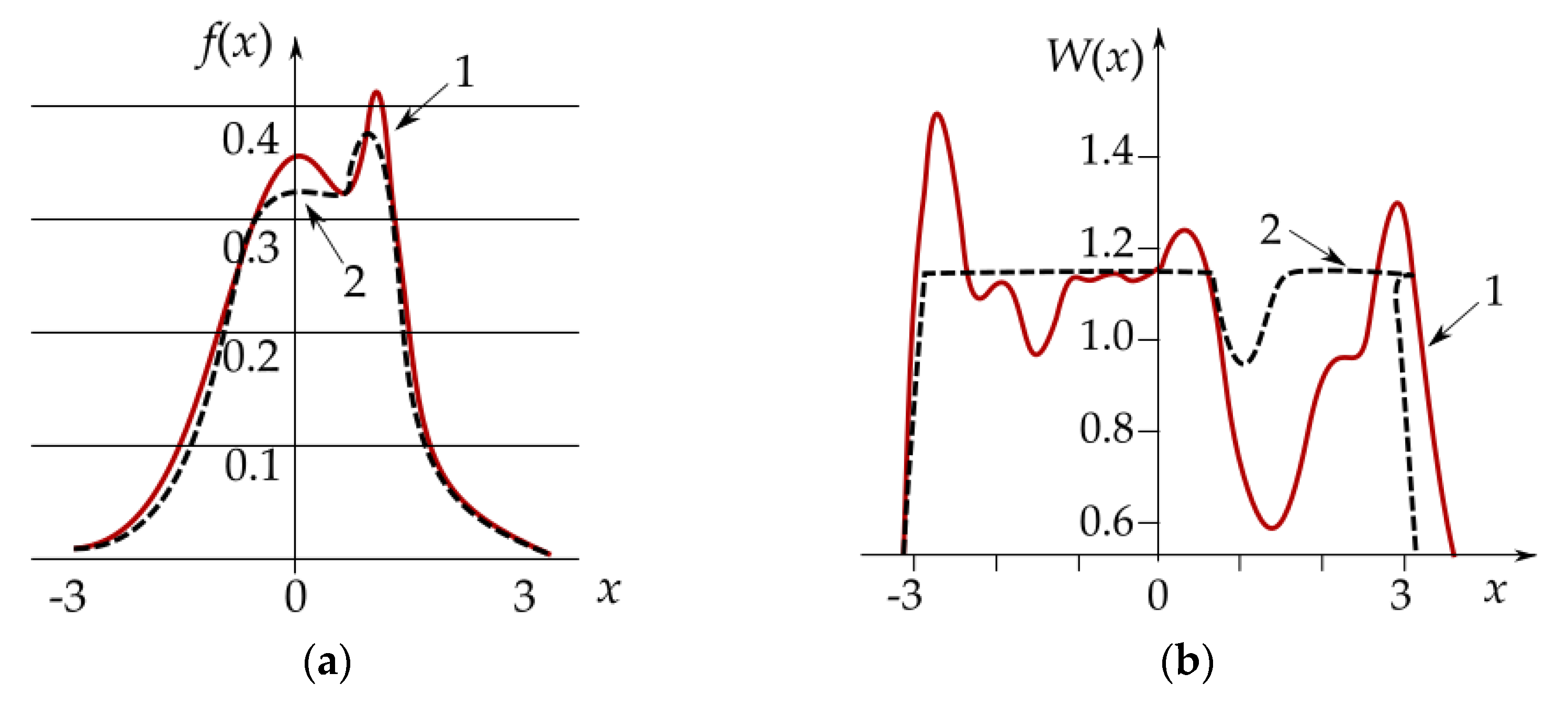
The appearance of Doppler acoustic radars (sodars) makes it possible to obtain information on the altitude profiles of wind velocity vector components with high spatial (up to several meters) and temporal resolution [4]. However, usually the outliers are detected and then eliminated from raw wind field data [5,6]. Thus, in [7], various outlier detection and elimination methods were analyzed, and the conclusion was drawn that in the previous works, outliers were simply removed and considered as missing data. In [8], a visual inspection method was used to eliminate the outliers. In this case, the information on the outliers and their contribution to the kinetic wind energy in the ABL was completely lost.

In the present work, we succeeded in analyzing the spatiotemporal dynamics of kinetic wind energy with and without allowance being made for the kinetic energy of outliers. We first represented the distribution $F(\mathsf{\zeta },\overrightarrow{\mathsf{\theta }})$ as a mixture of distributions $G(\mathsf{\zeta },\overrightarrow{\mathsf{\theta }})$ and $H(\mathsf{\zeta })$; we separated the contributions of the mean kinetic energy and the kinetic energy of the outliers, and estimated the latter using robust parametric, semiparametric, and semi-nonparametric algorithms developed by us.

We studied the diurnal hourly dynamics of kinetic wind energy in the lower 200 m layer of the atmosphere based on minisodar measurements of the wind velocity vector that obeys the distribution $F(\mathsf{\zeta },\overrightarrow{\mathsf{\theta }})$. Like all big data arrays, the minisodar measurements of altitude profiles of the wind velocity vectors have outliers and measurement errors. The integral estimate of the kinetic wind energy in the ABL $E_{\mathsf{\Sigma }}$ can be obtained from sample means and variances of the vertical profiles of the wind velocity vectors. To estimate the energy of the mean wind velocity, the unbiased, consistent, and effective estimates of the parameters of distribution $G(\mathsf{\zeta },\overrightarrow{\mathsf{\theta }})$ should be obtained, based on the measured vertical profiles of the wind velocity vector with the distribution $F(\mathsf{\zeta },\overrightarrow{\mathsf{\theta }})$. This can be achieved by using robust estimates of the parameters of the distribution $F(\mathsf{\zeta },\overrightarrow{\mathsf{\theta }})$.

Robust statistics is an actively developing branch of mathematics [8,9]. At present, different methods (including subjective ones) of obtaining robust estimates are proposed based on the minimization of various robustness criteria. Thus, in works [9,10,11], the criteria of minimizing the maximum asymptotic bias and the maximum variance were proposed. The advantages and disadvantages of the criterion of minimizing the maximum entropy were analyzed in [6,9]. The criteria of the maximum robustness and of the maximum distance were used for the minimum distance (MD) estimates in works [11,12]. The adaptive estimators were studied in works [6,11]. For example, for the shear parameter, about 50 different robust estimates were used, for example, based on robust M-estimators [11,13], regression credibility [14], or robust linear regression models [15]. This is obviously caused by the fact that in robust statistics, there is no established robustness criterion, unlike the efficiency criterion in classical mathematical statistics [16].

First, the robustness and efficiency criteria turned out to be contradictory, which stimulated the application of the robust estimates with intermediate characteristics (for example, the MD and Hellinger distance estimates [10,11] and the adaptive estimates [6,11]). Second, for the asymmetric outlier characteristics typical of the ABL [6,12,17,18], the robust estimates are biased and inconsistent [6,19]. Third, methods for obtaining the robust estimates are aimed at the removal of external outliers distant from the bulk of observations, whereas the presence of internal outliers can lead to essential errors in decision-making. All these problems stimulate the development of new robust, efficient algorithms for a wide class of outlier distributions, including asymmetric distributions and distributions with internal outliers. Such algorithms should adapt to the priori distributions. In the present work, robust algorithms are synthesized by the maximum likelihood method that converge to the effective algorithms for the inhomogeneous minisodar measurement data.

Unfortunately, real measurement data usually do not fit the mathematical models on which mathematical statistics heavily relies. Their processing requires solutions of a number of mathematical problems by robust nonparametric statistical methods [6]. Indeed, the problems of studying the spatiotemporal dynamics of kinetic wind energy in the ABL depend significantly on prior information on the distributions $F(\mathsf{\zeta },\overrightarrow{\mathsf{\theta }})$, $G(\mathsf{\zeta },\overrightarrow{\mathsf{\theta }})$, and $H\left(\mathsf{\zeta }\right)$. They can be divided into different classes: parametric (when $F(\mathsf{\zeta },\overrightarrow{\mathsf{\theta }})$, $G(\mathsf{\zeta },\overrightarrow{\mathsf{\theta }})$, and $H(\mathsf{\zeta })$ are parameterized to within unknown parameters $\overrightarrow{\mathsf{\theta }}$), semiparametric (when $F(\mathsf{\zeta },\overrightarrow{\mathsf{\theta }})$ and $G(\mathsf{\zeta },\overrightarrow{\mathsf{\theta }})$ are parameterized, and the form of $H(\mathsf{\zeta })$ is unknown), and semi-nonparametric (when the forms of $F(\mathsf{\zeta },\overrightarrow{\mathsf{\theta }})$, $G(\mathsf{\zeta },\overrightarrow{\mathsf{\theta }})$, and $H(\mathsf{\zeta })$ are unknown) problems of robust statistics [6]. As to the prior distribution $G(\mathsf{\zeta },\overrightarrow{\mathsf{\theta }})$, from physical considerations, most researchers think that it belongs to the class of symmetric normal-type distributions with light or medium tails [1,2,3]. The dynamics of the atmosphere in the ABL depends on many significant and not always measurable parameters. In this regard, the distribution $F(\mathsf{\zeta },\overrightarrow{\mathsf{\theta }})$, representing a mixture of the distributions $G(\mathsf{\zeta },\overrightarrow{\mathsf{\theta }})$ and $H(\mathsf{\zeta })$, should be referred to the nonparametric class. Traditionally, this class of problems is of great interest to scientists and has a century-old solution history [20,21]. Typical robust problems belong to the class of semiparametric statistics, provided that the fraction ε and the distribution of the outliers $H(\mathsf{\zeta })$ are unknown. In this case, the problem arises: how many sample observations, and from which side, should be trimmed to ensure the stability of the solutions obtained [12,17,20,21]. For example, symmetric trimming provides unbiased estimates for the symmetric distributions $G(\mathsf{\zeta },\overrightarrow{\mathsf{\theta }})$ and eliminates remote outliers [12,17], but the application of these procedures for asymmetric internal outliers leads to biased and ineffective estimates [6]. The semi-nonparametric problems for the unknown forms of $F(\mathsf{\zeta },\overrightarrow{\mathsf{\theta }})$, $G(\mathsf{\zeta },\overrightarrow{\mathsf{\theta }})$, and $H(\mathsf{\zeta })$ were not considered within the framework of robust statistics [6,12]. This is due to the fact that, for the unknown forms of the distributions $G(\mathsf{\zeta },\overrightarrow{\mathsf{\theta }})$ and $H(\mathsf{\zeta })$, the formal problem arises in the assessment of their differences. On the other hand, it should be noted that although the forms of distributions of the majority of observations $G(\mathsf{\zeta },\overrightarrow{\mathsf{\theta }})$ and outliers $H(\mathsf{\zeta })$ are unknown, researchers usually implicitly use some additional prior information concerning these distributions (their semi-nonparametric forms) to distinguish them. For example, the information on the class of distributions $H(\mathsf{\zeta })$ with external (internal) symmetric (asymmetric) outliers, and on the normal symmetric distributions $G(\mathsf{\zeta },\overrightarrow{\mathsf{\theta }})$ with light or medium tails, is often implicitly implied and allows symmetric trimming to be performed at a level of $2\mathsf{\sigma }$. The wind outliers, including wind gusts, are investigated using the skewness and kurtosis of their distributions [17,18]. This additional information on the distributions should be normalized and taken into account [22,23] to synthesize robust semi-nonparametric algorithms [12]. Hence, to estimate the kinetic wind energy components in the ABL from inhomogeneous data samples with the distribution $F(\mathsf{\zeta },\overrightarrow{\mathsf{\theta }})$, effective robust algorithms for the processing of experimental data with different levels of prior uncertainty should be developed.

In the present work, new robust parametric, semiparametric, and semi-nonparametric algorithms of the weighted maximum likelihood method are used to process experimental data with different levels of a priori statistical uncertainty to estimate the kinetic wind energy components in the ABL. The robust estimates of the total kinetic wind energy with and without allowance for the contribution of the outliers and of their difference equal to the kinetic wind energy of the outliers are obtained by postprocessing the measurements with an AV4000 minisodar [4].

The problem solved in the present work is formulated in Section 2 below. Section 3 describes the robust parametric algorithms and their application for estimating kinetic wind energy with and without allowance for the contribution of the outliers. In Section 4, the robust semiparametric algorithms are described and the results of their application are given. The kinetic wind energy with allowance for the contribution of the outliers and its mean and the turbulence components are presented together with the kinetic energy of the outliers retrieved by postprocessing of minisodar measurements. In the Conclusion, the main obtained results are given.

2. Problem Formulation

The kinetic wind energy in the ABL $E_{\mathsf{\Sigma }}=m{V}^2/2$ is determined by the energy of the motion of air masses—the wind energy. Below, we present the kinetic energy in the ABL reduced to unit air mass $E=E_{\mathsf{\Sigma }}/m$ and measured in m²/s² (m²/s² = J/kg) [24]. It is natural that the regularities in the spatiotemporal behavior of the reduced kinetic energy will fully refer to the total kinetic energy. For this reason, we use the term kinetic energy for the kinetic energy per unit air mass. It is equal to the sum of two components: the mean kinetic energy E_M, associated with the mean wind velocity $\overline{V}$, and the turbulence kinetic energy E_T, associated with the wind velocity variance ${\mathsf{\sigma }}^2$. Following [24], we can write:

$$\begin{array}{c}E=(E_M+E_T)/m=\frac{1}{2}\left({\overline{V}}^2+{\mathsf{\sigma }}^2\right),\\ {\displaystyle E_M=\frac{1}{2}(V_x^2+V_y^2+V_z^2),}\\ {\displaystyle E_T=\frac{1}{2}({\mathsf{\sigma }}_x^2+{\mathsf{\sigma }}_y^2+{\mathsf{\sigma }}_z^2),}\end{array}$$

(1)

where ${\overline{V}}_x$, ${\overline{V}}_y$, and ${\overline{V}}_z$ are mean values of the x, y, and z components of the wind velocity, and ${\mathsf{\sigma }}_x^2$, ${\mathsf{\sigma }}_y^2$, and ${\mathsf{\sigma }}_z^2$ are their variances. The wind vector $V(x,t,z)=\left(V_x,V_y,V_z\right)$ is a non-stationary random process. At a fixed altitude z, we consider the quasi-stationary interval $T$, and for $t\in T$, represent the process $V(x,t,z)$ as a superposition of the process $V_0$, stationary in a broad sense, with the prior distribution $G(\mathsf{\zeta },\overrightarrow{\mathsf{\theta }})$ characterizing the ordered movement of air masses, and the fraction ε of the outliers $V_{\mathrm{out}}$ with the distribution $H(\mathsf{\zeta })$ characterizing the inhomogeneous movement of air masses. As a convenient probabilistic model of the real distributions $F(\mathsf{\zeta },\overrightarrow{\mathsf{\theta }})$ used for studying the ABL, we take the mixture of the distributions $G(\mathsf{\zeta },\overrightarrow{\mathsf{\theta }})$ and $H(\mathsf{\zeta })$ that satisfies the regularity conditions. We consider that these models approximately coincide with the prior distribution $G(\mathsf{\zeta },\overrightarrow{\mathsf{\theta }})$ characterizing the ordered movement of air masses for $t\in T$ [1]. For this model, the energy of movement of air masses in the ABL, E is the sum of two components $E=E_{{}^0}+E_{{}^{\mathrm{out}}}$, where $E_{{}^0}$ is the energy of the stationary process, and $E_{{}^{\mathrm{out}}}$ is the energy of the outliers. With an allowance for Formula (1), we can write $E_{M0}=\frac{1}{2}{({\overline{V}}_0)}^2$, $E_{T0}=\frac{1}{2}{({\mathsf{\sigma }}_0)}^2$, $E_{M\mathrm{out}}=\frac{1}{2}{({\overline{V}}_{\mathrm{out}})}^2$, and $E_{T\mathrm{out}}=\frac{1}{2}{({\mathsf{\sigma }}_{\mathrm{out}})}^2$.

We studied the kinetic wind energy characteristics in the ABL by postprocessing the minisodar measurements of the x, y, and z components of the wind velocity $V_x(z_j,t_k)$, $V_y(z_j,t_k)$, and $V_z(z_j,t_k)$ in the jth strobe at altitude $z_j$ in the kth measurement series started at time $t_k$ during observation time T. We considered N observations (samples) $V_{xi}(z_j,t_k)$, $V_{yi}(z_j,t_k)$, and $V_{zi}(z_j,t_k)$, $i=1,\dots ,N$, during observation time T. Based on these samples, it is required to obtain unbiased, consistent estimates $({\widehat{E}}_M,{\widehat{E}}_T)$, $({\widehat{E}}_{M0},{\widehat{E}}_{T0})$, and $({\widehat{E}}_{M\mathrm{out}},{\widehat{E}}_{T\mathrm{out}})$ of the processes $V$, $V_0$, and $V_{\mathrm{out}}$.

The unbiased consistent estimate $\widehat{E}=({\widehat{E}}_M,{\widehat{E}}_T)$ averaged over the observation period T started at time $t_k\in T$ is equal to the mean and variance of the samples $V_{xi}(z_j,t_k)$, $V_{yi}(z_j,t_k)$, and $V_{zi}(i,z_j,t_k)$, $i=1,\dots ,N$. The unbiased and consistent estimates of ${\widehat{E}}_0=({\widehat{E}}_{M0},{\widehat{E}}_{T0})$ may be calculated from the unbiased and consistent estimates of the distribution $G(\mathsf{\zeta },\overrightarrow{\mathsf{\theta }})$ that may be obtained using the robust algorithms for the distribution $F(\mathsf{\zeta },\overrightarrow{\mathsf{\theta }})$ based on the samples $V_{xi}\left(z_j,t_k\right)$, $V_{yi}(z_j,t_k)$, $V_{zi}(z_j,t_k)$, $i=1,\dots ,N$, $t_k\in T$, from the distribution $F(\mathsf{\zeta },\overrightarrow{\mathsf{\theta }})$. Finally, the unbiased and consistent estimate of the outlier energy $({\widehat{E}}_{M\mathrm{out}},{\widehat{E}}_{T\mathrm{out}})$ is equal to the difference ${\widehat{E}}_{\mathrm{out}}=(\widehat{E}-{\widehat{E}}_0)$. Hence, the main problem is reduced to obtaining asymptotically unbiased, consistent, and effective estimates of the parameters of the distribution $G(\zeta ,\overrightarrow{\theta })$ based on the samples from the distribution $F(\mathsf{\zeta },\overrightarrow{\mathsf{\theta }})$; that is, the robust estimates for the distribution $F(\mathsf{\zeta },\overrightarrow{\mathsf{\theta }})$ based on prior information on the forms of the distributions $F(\mathsf{\zeta },\overrightarrow{\mathsf{\theta }})$, $G(\mathsf{\zeta },\overrightarrow{\mathsf{\theta }})$, and $H(\mathsf{\zeta })$ and their superpositions.

As already indicated above, robust statistics based on different robustness criteria cannot guarantee unbiased, consistent, and effective estimates of parameters, especially for asymmetric distributions $G(\mathsf{\zeta },\overrightarrow{\mathsf{\theta }})$ [6,10,11,19]. Considering the algorithms for robust estimation on different levels of prior information based on the weighted maximum likelihood method, we can formalize the problem. To simplify the derivation of the robust algorithms, we designated the samples $V_{xi}(z_j,t_k)$, $V_{yi}(z_j,t_k)$, and $V_{zi}(z_j,t_k)$, $i=1,\dots ,N$, by ${\overrightarrow{Z}}_N=({\mathsf{\zeta }}_1,\dots ,{\mathsf{\zeta }}_N)$. Let ${\overrightarrow{Z}}_N=({\mathsf{\zeta }}_1,\dots ,{\mathsf{\zeta }}_N)$ be the inhomogeneous sample of independent random variables with the distribution function $F(\mathsf{\zeta },\overrightarrow{\mathsf{\theta }})\in P$, where P is the class of distributions in the form of the mixture of the distributions satisfying the regularity conditions of the maximum likelihood method (MLM) [6,10,11]:

$$F(\mathsf{\zeta },\overrightarrow{\mathsf{\theta }})=(1-\mathsf{\epsilon })G(\mathsf{\zeta },\overrightarrow{\mathsf{\theta }})+\mathsf{\epsilon }H(\mathsf{\zeta }),$$

(2)

where $G(\mathsf{\zeta },\overrightarrow{\mathsf{\theta }})\in P_0$ is the a priori model of the distribution function, $H(\mathsf{\zeta })\in P$ is the outlier distribution, $\mathsf{\epsilon }\ge 0$ is the outlier fraction, and $\overrightarrow{\mathsf{\theta }}={({\mathsf{\theta }}_1,\dots ,{\mathsf{\theta }}_k)}^T$ is the unknown parameter vector of the distribution. We designated by $f(\mathsf{\zeta },\overrightarrow{\mathsf{\theta }})$, $g(\mathsf{\zeta },\overrightarrow{\mathsf{\theta }})$, and $h(\mathsf{\zeta })$ the corresponding distribution densities. Considering the problem of constructing the robust effective estimate ${\overrightarrow{\mathsf{\theta }}}_N^{\ast }={({\mathsf{\theta }}_{1N}^{\ast },\dots ,{\mathsf{\theta }}_{kN}^{\ast })}^T$ for the unknown parameter $\overrightarrow{\mathsf{\theta }}={({\mathsf{\theta }}_1,\dots ,{\mathsf{\theta }}_k)}^T$ of the prior distribution $G(\mathsf{\zeta },\overrightarrow{\mathsf{\theta }})$ from the inhomogeneous sample ${\overrightarrow{Z}}_N=({\mathsf{\zeta }}_1,\dots ,{\mathsf{\zeta }}_N)$ with the distribution $F(\mathsf{\zeta },\mathsf{\theta })\in P_{\mathsf{\theta }}$, the mathematical model (2) can be based on both parametric and nonparametric models of the distribution function and on their superpositions—semiparametric and semi-nonparametric models.

3. Robust Parametric Algorithms and Their Application for Estimating Kinetic Wind Energy

Let us consider the problem at the parametric level of prior uncertainty. For the sample ${\overrightarrow{Z}}_N=({\mathsf{\zeta }}_1,\dots ,{\mathsf{\zeta }}_N)$ with the distribution $F(\mathsf{\zeta },\overrightarrow{\mathsf{\theta }})$, we first derived the maximum likelihood estimate (MLE) ${\overrightarrow{\mathsf{\theta }}}_N^{\ast }$ in $F(\mathsf{\zeta },\overrightarrow{\mathsf{\theta }})$. By analogy with [5,8], it can be shown that the consistent asymptotically unbiased effective estimates ${\overrightarrow{\mathsf{\theta }}}_N^{\ast }={({\mathsf{\theta }}_{1N}^{\ast },\dots ,{\mathsf{\theta }}_{kN}^{\ast })}^T$ for the prior distribution $G(\mathsf{\zeta },\overrightarrow{\mathsf{\theta }})$ are determined from the system of estimation equations:

$$\frac{1}{N}{\displaystyle \sum _{i=1}^{N}U\left({\mathsf{\zeta }}_i,{\overrightarrow{\mathsf{\theta }}}_N^{\ast }\right)W\left({\mathsf{\zeta }}_i,{\overrightarrow{\mathsf{\theta }}}_N^{\ast }\right)}=0, j=\overline{1,k},$$

(3)

$$U_j(\mathsf{\zeta },{\overrightarrow{\mathsf{\theta }}}_N^{\ast })=\frac{\partial }{\partial {\mathsf{\theta }}_j}\ln g(\mathsf{\zeta },{\overrightarrow{\mathsf{\theta }}}_N^{\ast }){|}_{\mathsf{\theta }={\overrightarrow{\mathsf{\theta }}}_N^{\ast }},$$

(4)

$$W(\mathsf{\zeta },{\overrightarrow{\mathsf{\theta }}}_N^{\ast })=\frac{(1-\mathsf{\epsilon })g(\mathsf{\zeta },{\overrightarrow{\mathsf{\theta }}}_N^{\ast })}{f(\mathsf{\zeta },{\overrightarrow{\mathsf{\theta }}}_N^{\ast })}.$$

(5)

The estimates ${\overrightarrow{\mathsf{\theta }}}_N^{\ast }$ from the system of estimation Equation (3) are determined by iterations and are estimates of the weighted maximum likelihood method (WMLM). The efficiency of the estimates follows from the MLM, the unbiasedness of the estimates for $G(\mathsf{\zeta },\overrightarrow{\mathsf{\theta }})$ was shown in [12], and their robustness follows from the bounded variances provided with the weight functions $W(\mathsf{\zeta },{\overrightarrow{\mathsf{\theta }}}_N^{\ast })$ given by Equation (5).

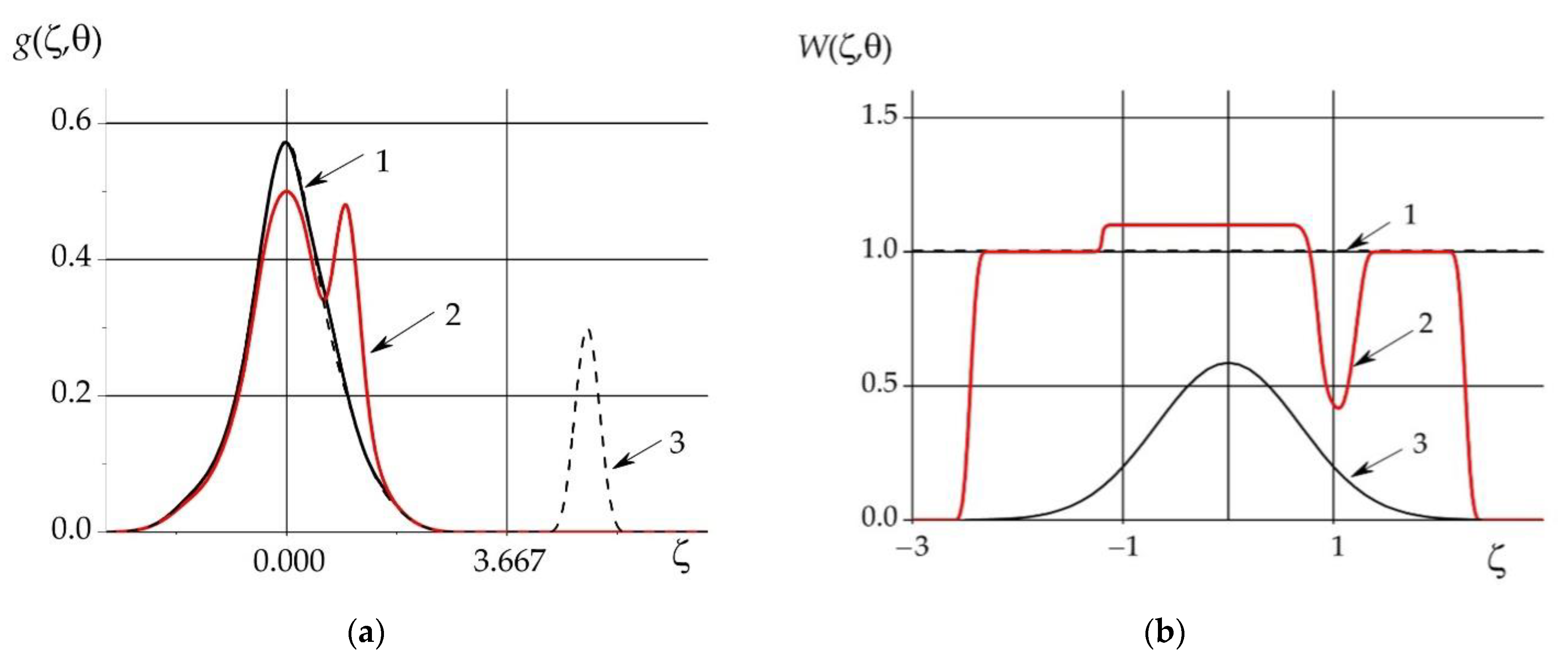
As an example, we considered the algorithms for robust estimates of the mean and variance $\overrightarrow{\mathsf{\theta }}=(\mathsf{\mu },s)$ of the prior normal distribution $G(\mathsf{\zeta },\overrightarrow{\mathsf{\theta }})$:

$$g(\mathsf{\zeta },u)=\frac{1}{s\sqrt{2\mathsf{\pi }}}\exp \left(-\frac{u^2}{2}\right),f(\mathsf{\zeta },u,\mathsf{\nu },\mathsf{\lambda })=(1-\mathsf{\epsilon })g(\mathsf{\zeta },u)+\mathsf{\epsilon }g(\mathsf{\zeta },\mathsf{\nu },\mathsf{\lambda }),$$

$$U_1(\mathsf{\zeta },u)=u,U_2(\mathsf{\zeta },u)=\left[u^2-1\right],W(\mathsf{\zeta },\mathsf{\nu },\mathsf{\lambda })=\frac{(1-\mathsf{\epsilon })g(\mathsf{\zeta },\mathsf{\mu },s)}{f(\mathsf{\zeta },\mathsf{\nu },\mathsf{\lambda })},u=\frac{\mathsf{\zeta }-\mathsf{\mu }}{s}.$$

(6)

The plots of the corresponding distribution densities, weight functions, and estimate functions for the normal distribution are shown in Figure 1 for the indicated outlier fractions.

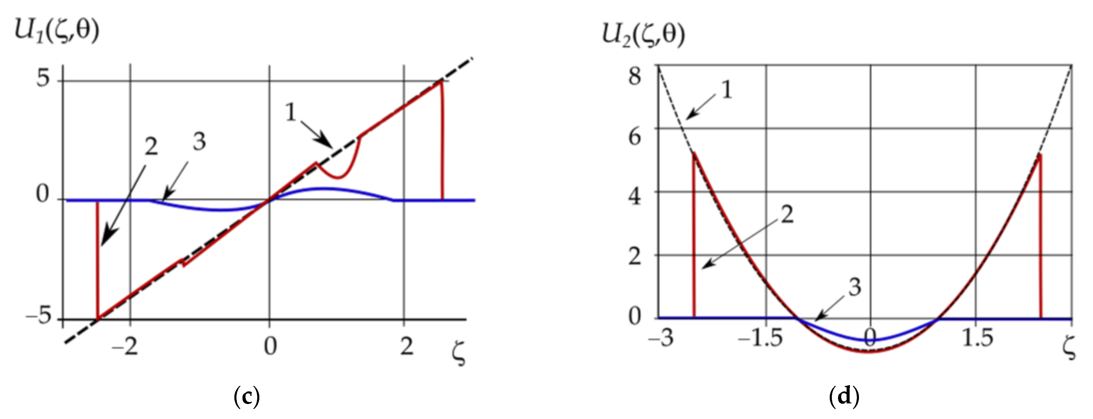
Figure 2a shows an example of the parametric estimates of the vertical profiles of the total kinetic wind energy without (E₀, the orange curve) and with an allowance for the contribution of the kinetic outlier energy (E, the blue curve) retrieved from measurements with the commercial triaxial Doppler monostatic minisodar AV4000 (Atmospheric Systems Corporation, Santa Clara, CA, USA) [4]; its sounding range was 5–200 m with vertical resolution Δz = 5 m. The acoustic antenna was an array of 50 loudspeakers used to both transmit and receive acoustic signals at a frequency of 4900 Hz. This loudspeaker array was electrically steered to generate three independent beams: one vertical and two others at elevation angles of 76° in two mutually orthogonal planes. The minisodar had a pulse repetition period of 4 s and a pulse duration of 60 ms. The minisodar provided one vertical signal profile in all three channels every 4 s, which was used to calculate the wind vector components V_x(z, t), V_y(z, t), and V_z(z, t), and their variances, ${\mathsf{\sigma }}_x^2(z,t)$, ${\mathsf{\sigma }}_y^2(z,t)$, and ${\mathsf{\sigma }}_z^2(z,t)$ from the well-known formulas for the Doppler frequency shifts. To investigate their dynamics, we sampled and processed 150 vertical profiles recorded from the beginning of each hour from 00:00 till 23:00 to obtain 10 min averages and to estimate the total kinetic wind energy E(z, t) and its components caused by the stationary air movement E₀(z, t) and the wind outliers E_out(z, t).

Continuous minisodar measurements were taken in the vicinity of Santa Clarita, CA, USA (34°23′29.9904″ N, 118°32′33.3096″ W) over a flat underlying surface without tall vegetation [25] from 10 to 17 September 2003. During the period of the measurements, the weather was dry, warm and sunny. Here, we postprocessed 10-min averaged minisodar measurements that started on 10 September at 12:00 LT, and at every hour from 00:00 till 23:00 on 16 September. The temperature during the period of measurements on 10 September was 23 °C, and the mean wind speed was 3.57 m/s. The maximum daytime temperature on 16 September was 25.7 °C, and the minimum temperature at night was 16 °C. The average wind velocity was 9.1 m/s.

From Figure 2, it can be seen that without the contribution of the kinetic outlier energy, the curve is quite smooth, whereas with an allowance made for this contribution, its layered structure can clearly be seen. It should also be noted that the atmospheric layers with strong turbulence were also pointed out by Shikhovtsev et al. in [26] and Bolbasova et al. in [27], where the maximum changes of the turbulence layer strengths were observed in the lower layer of the atmosphere at altitudes up to 70 m, and the diurnal variations of their altitudes were also indicated. The blue curve in Figure 2a also shows that local outlier layers were clearly manifested in the vertical profile of the total kinetic energy starting from an altitude of 50 m; moreover, the thickness of these layers remained practically unchanged to altitudes of 150 m. Above 150 m, the curves synchronously changed with altitude and had kinetic energy maxima at z = 175 m. This suggests that new robust algorithms [14] for the detection and selection of outliers of various origins in the observation samples at different levels of a priori statistical uncertainty are especially important for altitude ranges in which the kinetic outlier energy is significant. For this reason, of considerable interest are the physical reasons for the appearance of these features in the kinetic outlier energy. Figure 2b shows an example of the altitude profiles of the turbulence kinetic energy component E_T without (the orange curve) and with allowance for the contribution of the kinetic outlier energy (the blue curve). The comparison of Figure 2a,b demonstrates that, in this situation, the altitude behavior of the orange and blue curves differs quantitatively only in the layer below 25 m; above this altitude, they qualitatively agree. This suggests that at these altitudes, the predominant contribution to the total kinetic wind energy comes from the turbulence kinetic energy component.

In Figure 2a,b, the fairly smooth (orange) curves of the parametric estimates of the vertical profiles of the kinetic energy of stationary air motion, disregarding the contribution of the kinetic outlier energy, can be seen. Taking into account the contribution of the kinetic energy of outliers, the blue curves depict the fine structure of the altitude dependence of the total kinetic energy. This testifies that, in this case, attention should be focused on the kinetic energy of the outliers.

4. Robust Semiparametric Algorithms and Their Application for Estimating Kinetic Wind Energy

Let us consider the problem at the semiparametric level of prior uncertainty. In this case, it is assumed that $G(\mathsf{\zeta },\overrightarrow{\mathsf{\theta }})$ is known to within a finite number of the unknown parameters $\overrightarrow{\mathsf{\theta }}$, and the information on the outliers $\left\{\mathsf{\epsilon },H(\mathsf{\zeta })\right\}$, that is, on the form of the distribution function $H(\mathsf{\zeta })$ and, hence, $F(\mathsf{\zeta },\overrightarrow{\mathsf{\theta }})$ is unknown. For the sample ${\overrightarrow{Z}}_N=({\mathsf{\zeta }}_1,\dots ,{\mathsf{\zeta }}_N)$ from $F(\mathsf{\zeta },\overrightarrow{\mathsf{\theta }})$, we obtained the estimate ${\overrightarrow{\mathsf{\theta }}}_N$ by the maximum likelihood method. By analogy with [12], it is possible to show that the asymptotically effective (unbiased and consistent) estimates ${\overrightarrow{\mathsf{\theta }}}_N^{\ast }={({\mathsf{\theta }}_{1N}^{\ast },\dots ,{\mathsf{\theta }}_{kN}^{\ast })}^T$ of the WMLM for the prior distribution $G(\mathsf{\zeta },\overrightarrow{\mathsf{\theta }})$ are determined from the system of the estimation equations:

$$\frac{1}{N}{\displaystyle \sum _{i=1}^{N}U({\mathsf{\zeta }}_i,{\overrightarrow{\mathsf{\theta }}}_N^{\ast })W_N({\mathsf{\zeta }}_i,{\overrightarrow{\mathsf{\theta }}}_N^{\ast })=0}, j=\overline{1,k},$$

(7)

$$U_j(\mathsf{\zeta },{\overrightarrow{\mathsf{\theta }}}_N^{\ast })=\frac{\partial }{\partial {\mathsf{\theta }}_j}\ln g(\mathsf{\zeta },{\overrightarrow{\mathsf{\theta }}}_N^{\ast }){|}_{\mathsf{\theta }={\overrightarrow{\mathsf{\theta }}}_N^{\ast }},$$

(8)

$$W_N({\mathsf{\zeta }}_i,{\overrightarrow{\mathsf{\theta }}}_N^{\ast })=\frac{(1-\mathsf{\epsilon })g({\mathsf{\zeta }}_i,{\overrightarrow{\mathsf{\theta }}}_N^{\ast })}{f_N({\mathsf{\zeta }}_i,{\overrightarrow{\mathsf{\theta }}}_N^{\ast })},$$

(9)

$$f_N(\mathsf{\zeta })=\frac{1}{N{h}_N}{\displaystyle \sum _{i=1}^N}k\left(\frac{\mathsf{\zeta }-x_i}{h_N}\right),$$

(10)

where $f_N(\mathsf{\zeta })$ is the nonparametric estimate of the Parzen–Rosenblatt density, $k(u)$ is the kernel function, and $h_N$ is the bandwidth [6,8]. For $f_N(\mathsf{\zeta })$ to be consistent and unbiased, the following conditions must be satisfied: $\left\{k(u)=k(-u), {\displaystyle \underset{-\infty }{\overset{\infty }{\mathsf{\int }}}k(u)du}=1, h_N\to 0, N{h}_N\to \infty \mathrm{when} N\to \infty \right\}$.

The estimates ${\overrightarrow{\mathsf{\theta }}}_N^{\ast }$ are defined from the system of estimation Equation (8) by iterations. The efficiency of the estimates follows from the WMLM, and the unbiased and bounded variances of the estimates are provided by the weight functions $W_N({\mathsf{\zeta }}_i,{\overrightarrow{\mathsf{\theta }}}_N^{\ast })$ given by Equation (9). For example, for the normal distribution with the shear parameter $G(\mathsf{\zeta },\mathsf{\theta })$,

$$g(\mathsf{\zeta },\mathsf{\theta })=\frac{1}{\sqrt{2\mathsf{\pi }}\mathsf{\sigma }}\exp \left(-\frac{{(\mathsf{\zeta }-\mathsf{\theta })}^2}{2{\mathsf{\sigma }}^2}\right).$$

Estimation Equation (8) assumes the form

$${\displaystyle \sum _{i=1}^N({\mathsf{\zeta }}_i-{\mathsf{\theta }}_N)}W({\mathsf{\zeta }}_i,{\mathsf{\theta }}_N)=0,$$

$$W_N({\mathsf{\zeta }}_i,{\mathsf{\theta }}_N)=\frac{\exp \left(-\frac{{({\mathsf{\zeta }}_i-{\mathsf{\theta }}_N)}^2}{2{\mathsf{\sigma }}^2}\right)}{f_N({\mathsf{\zeta }}_i)},f_N(\mathsf{\zeta })=\frac{1}{N\sqrt{2\mathsf{\pi }}{h}_N}{\displaystyle \sum _{j=1}^N\exp \left(-\frac{1}{2}{\left(\frac{\mathsf{\zeta }-{\mathsf{\zeta }}_j}{h_N}\right)}^2\right)}.$$

(11)

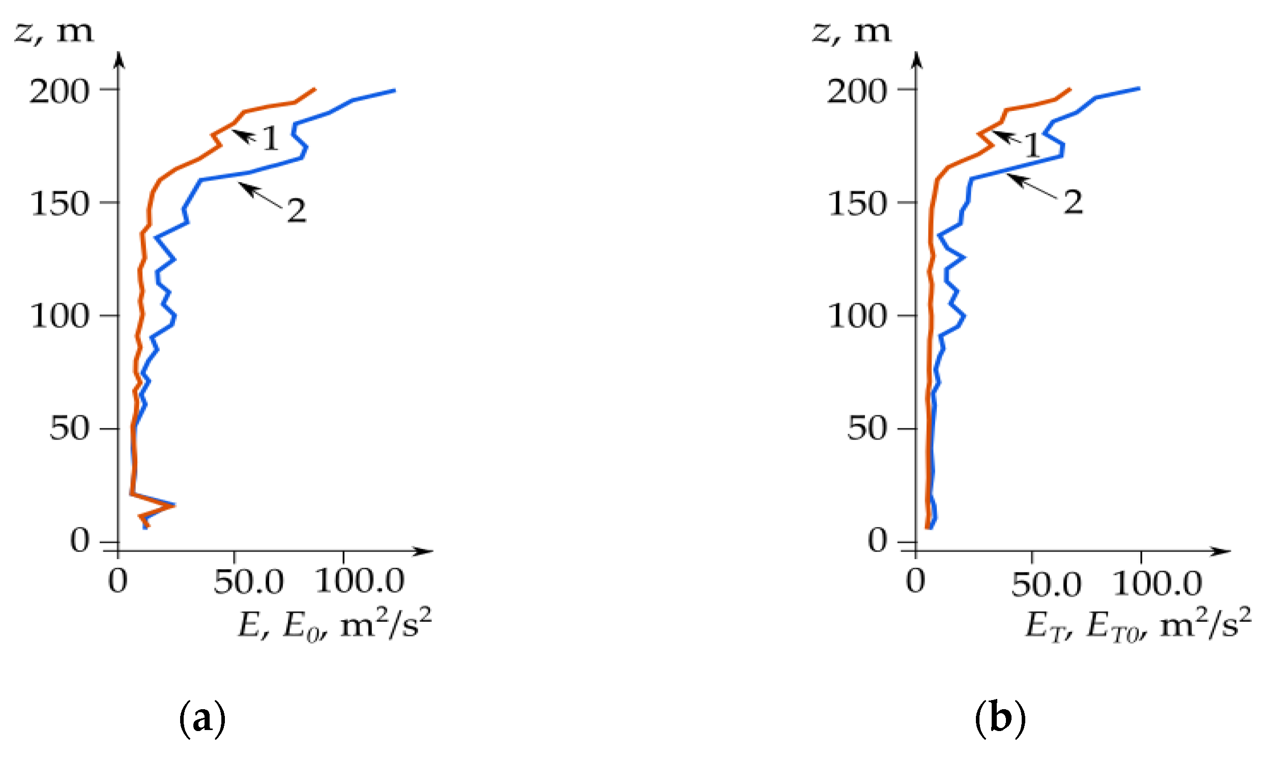
In Figure 3, the results of modeling are shown for observations of the superposition of the normal distributions of asymmetric internal outliers with $\mathsf{\theta }=0, \mathsf{\epsilon }=0.1, \mathsf{\mu }=1, \mathrm{and} \mathsf{\lambda }=0.2$

$$f(\mathsf{\zeta },\mathsf{\theta })=\frac{0.9}{\sqrt{2\mathsf{\pi }}}\exp \left[-\frac{{\mathsf{\zeta }}^2}{2}\right]+\frac{0.1}{\sqrt{2\mathsf{\pi }}\mathsf{\lambda }}\exp \left[-\frac{{(\mathsf{\zeta }-\mathsf{\mu })}^2}{2\mathsf{\lambda }}\right].$$

To determine the kinetic energy $E_0$ of the stationary process, we needed to determine the mean $\overline{X}(\overrightarrow{\mathsf{\theta }})$ and variance ${\mathsf{\sigma }}^2(\overrightarrow{\mathsf{\theta }})$ of the distribution $G(\mathsf{\zeta },\overrightarrow{\mathsf{\theta }})$:

$$\overline{X}(\overrightarrow{\mathsf{\theta }})={\displaystyle \underset{-\infty }{\overset{\infty }{\mathsf{\int }}}\mathsf{\zeta }\cdot g(\mathsf{\zeta },\overrightarrow{\mathsf{\theta }})}d\mathsf{\zeta },{\mathsf{\sigma }}^2(\overrightarrow{\mathsf{\theta }})={{\displaystyle \underset{-\infty }{\overset{\infty }{\mathsf{\int }}}\left(\mathsf{\zeta }-\overline{X}(\overrightarrow{\mathsf{\theta }})\right)}}^2\cdot g(\mathsf{\zeta },\overrightarrow{\mathsf{\theta }})d\mathsf{\zeta }.$$

(12)

Defining from Equations (8)–(10) the asymptotically effective robust estimates of the parameters ${\overrightarrow{\mathsf{\theta }}}_N^{\ast }={({\mathsf{\theta }}_{1N}^{\ast },\dots ,{\mathsf{\theta }}_{kN}^{\ast })}^T$ and substituting them into Equation (8), we obtained for $\overline{X}(\overrightarrow{\mathsf{\theta }})$ and ${\mathsf{\sigma }}^2(\overrightarrow{\mathsf{\theta }})$ the asymptotically effective robust estimates of the mean ${\overline{X}}_N({\overrightarrow{\mathsf{\theta }}}_N^{\ast })$ and variance ${\mathsf{\sigma }}_N^2({\overrightarrow{\mathsf{\theta }}}_N^{\ast })$ and determined on their basis the kinetic energy $E_0$ of the stationary process.

5. Robust Semi-Nonparametric Algorithms and Their Application for Estimation of Kinetic Wind Energy

Let us consider the class of semi-nonparametric problems of robust statistics in which the information on the prior distribution $G(\mathsf{\zeta },\overrightarrow{\mathsf{\theta }})$ and the outliers $\left\{H(\mathsf{\zeta }),\mathsf{\epsilon }\right\}$; that is, on the forms of the distribution functions $H(\mathsf{\zeta })$, $G(\mathsf{\zeta },\overrightarrow{\mathsf{\theta }})$ and, hence, $F(\mathsf{\zeta },\overrightarrow{\mathsf{\theta }})$ is unknown. As the parameters $\overrightarrow{\mathsf{\theta }}$ of this nonparametric class of distributions $G(\mathsf{\zeta },\overrightarrow{\mathsf{\theta }})$, the shear and scale parameters can be considered and, in general, some functionals of $G(\mathsf{\zeta },\overrightarrow{\mathsf{\theta }})$. Note that though the forms of distribution of the majority of observations $G(\mathsf{\zeta },\overrightarrow{\mathsf{\theta }})$ and of the outliers $H(\mathsf{\zeta })$ are unknown, the researchers usually use some additional prior information on these distributions which allows them to be distinguished. We formalized this additional prior information. It is known a priori that $G(\mathsf{\zeta },\mathsf{\theta })\in {\tilde{P}}_{0\mathsf{\theta }}$, where ${\tilde{P}}_{0\mathsf{\theta }}$ is a nonparametric class of continuous functions satisfying to the conditions

$$S_i={\displaystyle \mathsf{\int }{\mathsf{\psi }}_i(x)dG(x,\mathsf{\theta })}=0,\hspace{1em}i=1,\dots ,r,$$

(13)

where the functions ${\mathsf{\psi }}_1,\dots ,{\mathsf{\psi }}_r$ are known. The assignment of the prior information in the form of Equation (13) allows one to consider a wide spectrum of information on $G(\mathsf{\zeta },\mathsf{\theta })$ of both quantitative and qualitative character [22,23]. Taking into account prior information (13), the modified nonparametric estimate of the Parzen–Rosenblatt density ${\tilde{g}}_N(\mathsf{\zeta },\mathsf{\theta })$ can be constructed [22,23]:

$${\tilde{g}}_N(\mathsf{\zeta })=\frac{1}{N}{\displaystyle \sum _{i=1}^N\frac{1}{h_N}}k(\frac{\mathsf{\zeta }-{\mathsf{\zeta }}_i}{h_N})\left[1-‖\frac{1}{N}{\displaystyle \sum _{i=1}^N{\mathsf{\psi }}_l({\mathsf{\zeta }}_i)}‖{\mathsf{\Lambda }}_N^{-1}{‖\frac{1}{N}{\displaystyle \sum _{i=1}^N{\mathsf{\psi }}_j({\mathsf{\zeta }}_i)}‖}^T\right].$$

(14)

The estimate ${\tilde{g}}_N(\mathsf{\zeta })$ is asymptotically unbiased, consistent, and $\sqrt{N{h}_N}\left[{\tilde{g}}_N(\mathsf{\zeta })-E{\tilde{g}}_N(\mathsf{\zeta })\right]$ has the asymptotically normal distribution [22,23].

Let us define the WMLM estimation equation for $G(\mathsf{\zeta },\mathsf{\theta })\in {\tilde{P}}_{0\mathsf{\theta }}$ in the form

$$\frac{1}{N}{\displaystyle \sum _{i=1}^N{\tilde{\mathsf{\phi }}}_N({\mathsf{\zeta }}_i,{\mathsf{\theta }}_N)=0},$$

(15)

where the estimation function ${\tilde{\mathsf{\phi }}}_N(\mathsf{\zeta },\mathsf{\theta })$ is

$${\tilde{\mathsf{\phi }}}_N(\mathsf{\zeta },\mathsf{\theta })=\frac{\partial }{\partial \mathsf{\theta }}\ln {\tilde{g}}_N(\mathsf{\zeta },\mathsf{\theta })\frac{{\tilde{g}}_N(\mathsf{\zeta },\mathsf{\theta })}{f_N(\mathsf{\zeta },\mathsf{\theta })}=\tilde{U}(\mathsf{\zeta },\mathsf{\theta }){\tilde{W}}_N(\mathsf{\zeta },\mathsf{\theta }),$$

(16)

$\tilde{U}(\mathsf{\zeta },\mathsf{\theta })$ is the function of the MLE contribution for $\tilde{G}(\mathsf{\zeta },\mathsf{\theta })$, ${\tilde{W}}_N(\mathsf{\zeta },\mathsf{\theta })$ is the weight function:

$${\tilde{W}}_N(\mathsf{\zeta },\mathsf{\theta })=\frac{(1-\mathsf{\epsilon }){\tilde{g}}_N(\mathsf{\zeta },\mathsf{\theta })}{f_N(\mathsf{\zeta },\mathsf{\theta })},$$

(17)

and $f_N(\mathsf{\zeta })$ is the nonparametric estimate of the Parzen–Rosenblatt density given by Equation (10). Formulas (15)–(17) define the adaptive nonparametric estimate (ANE) ${\tilde{\mathsf{\theta }}}_N^{\ast }$ of the WMLM.

For example, let $G(\mathsf{\zeta },\mathsf{\theta })\in {\tilde{P}}_{0\mathsf{\theta }}$ be a symmetric function of the parameter $\mathsf{\theta }$. The modified nonparametric estimate of the Parzen–Rosenblatt density takes the form [22,23]

$${\tilde{g}}_N(\mathsf{\zeta },\mathsf{\theta })=\frac{1}{2}\left[\frac{1}{N{h}_N}{\displaystyle \sum _{j=1}^{N}k\left(\frac{\mathsf{\zeta }-{\mathsf{\zeta }}_j}{h_N}\right)}-\frac{1}{N{h}_N}{\displaystyle \sum _{i=1}^{N}k\left(\frac{2\mathsf{\theta }-\mathsf{\zeta }-{\mathsf{\zeta }}_i}{h_N}\right)}\right].$$

(18)

The estimate ${\tilde{g}}_N(\mathsf{\zeta },\mathsf{\theta })$ is asymptotically unbiased, consistent, and has the minimal root-mean square error on the nonparametric class of distributions ${\tilde{P}}_{0\mathsf{\theta }}$.

Let $\mathsf{\beta }$ be the unknown parameter of $G(\mathsf{\zeta },\mathsf{\theta })\in {\tilde{P}}_{0\mathsf{\theta }}$ in the form:

$$\mathsf{\beta }={\displaystyle \int \rho (x,\mathsf{\theta }})dG(x,\mathsf{\theta })\mathrm{or}{\displaystyle \int \rho (x,\mathsf{\theta }})dG(x,\mathsf{\theta })-\mathsf{\beta }=0$$

(19)

To derive the robust estimate ${\mathsf{\beta }}_N$ of the parameter β, consider the estimation equation in the form:

$$\frac{1}{N}{\displaystyle \sum _{i=1}^N{\tilde{\mathsf{\omega }}}_N({\mathsf{\zeta }}_i,{\mathsf{\theta }}_N)=0},$$

(20)

where the estimation function ${\tilde{\mathsf{\phi }}}_N(\mathsf{\zeta },\mathsf{\theta })$ has the form:

$${\tilde{\mathsf{\omega }}}_N(\mathsf{\zeta },\mathsf{\theta })=(\mathsf{\rho }(\mathsf{\zeta },\mathsf{\theta })-\mathsf{\beta }){\tilde{W}}_N(\mathsf{\zeta },\mathsf{\theta })$$

(21)

${\tilde{W}}_N(\mathsf{\zeta },\mathsf{\theta })=\frac{{\tilde{g}}_N(\mathsf{\zeta },\mathsf{\theta })}{f_N(\mathsf{\zeta },\mathsf{\theta })}$ is the weight function, $f_N(\mathsf{\zeta })$ is the nonparametric estimate of the Parzen–Rosenblatt density given by Equation (10), and ${\tilde{g}}_N(\mathsf{\zeta },\mathsf{\theta })$ is the modified nonparametric estimate of the Parzen–Rosenblatt density. Formulas (20) and (21) define the robust semi-nonparametric estimate β_N of the parameter β. A mathematical analysis of these estimates is beyond the scope of the present work. Note only that they are asymptotically unbiased and efficient for the distribution $G(\mathsf{\zeta },\mathsf{\theta })\in {\tilde{P}}_{0\mathsf{\theta }}$, provided that the sample ${\overrightarrow{{\rm Z}}}_N=({\mathsf{\zeta }}_1,\dots ,{\mathsf{\zeta }}_N)$ is from $F(\mathsf{\zeta },\overrightarrow{\mathsf{\theta }})$.

For example, let $G(\mathsf{\zeta },\mathsf{\theta })\in {\tilde{P}}_{0\mathsf{\theta }}$ be the class of symmetric functions of the shear parameter θ. Let us designate by $(\mu ,s)$ the average and variance of $G(\mathsf{\zeta },\mathsf{\theta })$. In this case, the estimation equations for the robust nonparametric estimates $({\mathsf{\mu }}_N,s_N)$ and normal kernel function (7) take the following forms:

$${\displaystyle \sum _{i=1}^N{\displaystyle \sum _{j=1}^N({\mathsf{\mu }}_N-t_{ij})\frac{{\tilde{g}}_N\left(-\frac{{\left({\mathsf{\mu }}_N-t_{ij}\right)}^2}{2{\mathsf{\sigma }}_N^2}\right)}{f_N({\mathsf{\zeta }}_i)}}}=0,$$

$${\displaystyle \sum _{i=1}^N{\displaystyle \sum _{j=1}^N{({\mathsf{\sigma }}_N-t_{ij})}^2\frac{{\tilde{g}}_N\left(-\frac{{\left({\mathsf{\mu }}_N-t_{ij}\right)}^2}{2{\mathsf{\sigma }}_N^2}\right)}{f_N({\mathsf{\zeta }}_i)}}}=0$$

where $t_{i,j}=\frac{{\mathsf{\zeta }}_i+{\mathsf{\zeta }}_j}{2}$ are the Walsh half-sums and ${\tilde{g}}_N(\mathsf{\zeta },\mathsf{\theta })$ is defined by Formula (10). The estimates are determined by iterations. The estimates of the kinetic energies of the stationary process without outliers, $E_0$, and with the outliers, $E_{\mathrm{out}}$, were obtained using these formulas.

Table 1. Semi-nonparametric estimates of the kinetic wind energy components.

Altitude z, m	10	20	30	40	50	60	70	80	90	100
E0, m2/s2	8.03	3.29	4.40	4.13	3.76	5.82	6.47	5.60	6.75	8.03
E, m2/s2	9.62	3.34	4.62	4.33	4.17	9.25	11.50	10.60	12.68	23.68
Eout, m2/s2	1.59	0.05	0.22	0.20	0.41	3.43	5.03	5.0	5.93	15.65
Altitude z, m	110	120	130	140	150	160	170	180	190	200
E0, m2/s2	8.93	6.61	8.36	11.0	11.7	16.6	34.76	40.13	53.94	85.83
E, m2/s2	20.73	15.46	16.8	28.83	28.09	35.39	80.35	76.71	92.58	121.80
Eout, m2/s2	11.8	8.85	8.44	17.83	16.39	18.79	45.59	36.58	38.64	35.97

presents the semi-nonparametric estimates of the altitude dependence of the kinetic wind energy without outliers, $E_0$, the kinetic wind energy with an allowance for the contribution of the outliers, E, and their difference $E-E_0=E_{\mathrm{out}}$ equal to the kinetic energy of the outliers obtained by the postprocessing of the minisodar measurements.

Consider first the semi-nonparametric estimates $E_0$ of the kinetic energy without outliers. Their nearly monotonic increase with altitude could be easily traced from 20 to 200 m. The large E₀ value at z = 10 m is apparently caused by the effect of the underlying surface. The rate of E₀ growth increased with altitude starting from z = 150 m. Our statistical analysis of the altitude behavior of the total kinetic energy E with an allowance for the contribution of the kinetic energy of outliers revealed the following. The E values differred only slightly from the corresponding E₀ values at altitudes up to 50 m, that is, in this altitude range, the contribution of the kinetic outlier energy to the total kinetic energy was low. The situation radically changed above 50 m. An essential nonmonotonic increase in E values was observed with a further increase in the altitude, accompanied by considerable deviations from the monotonic dependence.

As to the altitude dependence of the kinetic energy of outliers E_out, it was low at altitudes z ≤ 50 m. Its increase at z = 10 m was caused by the effect of the underlying surface. From 50 to 170 m, the nonmonotonic increase in E_out was observed together with increasing E_out values between 100 and 110 m. Above 170 m, a certain decrease in E_out was observed.

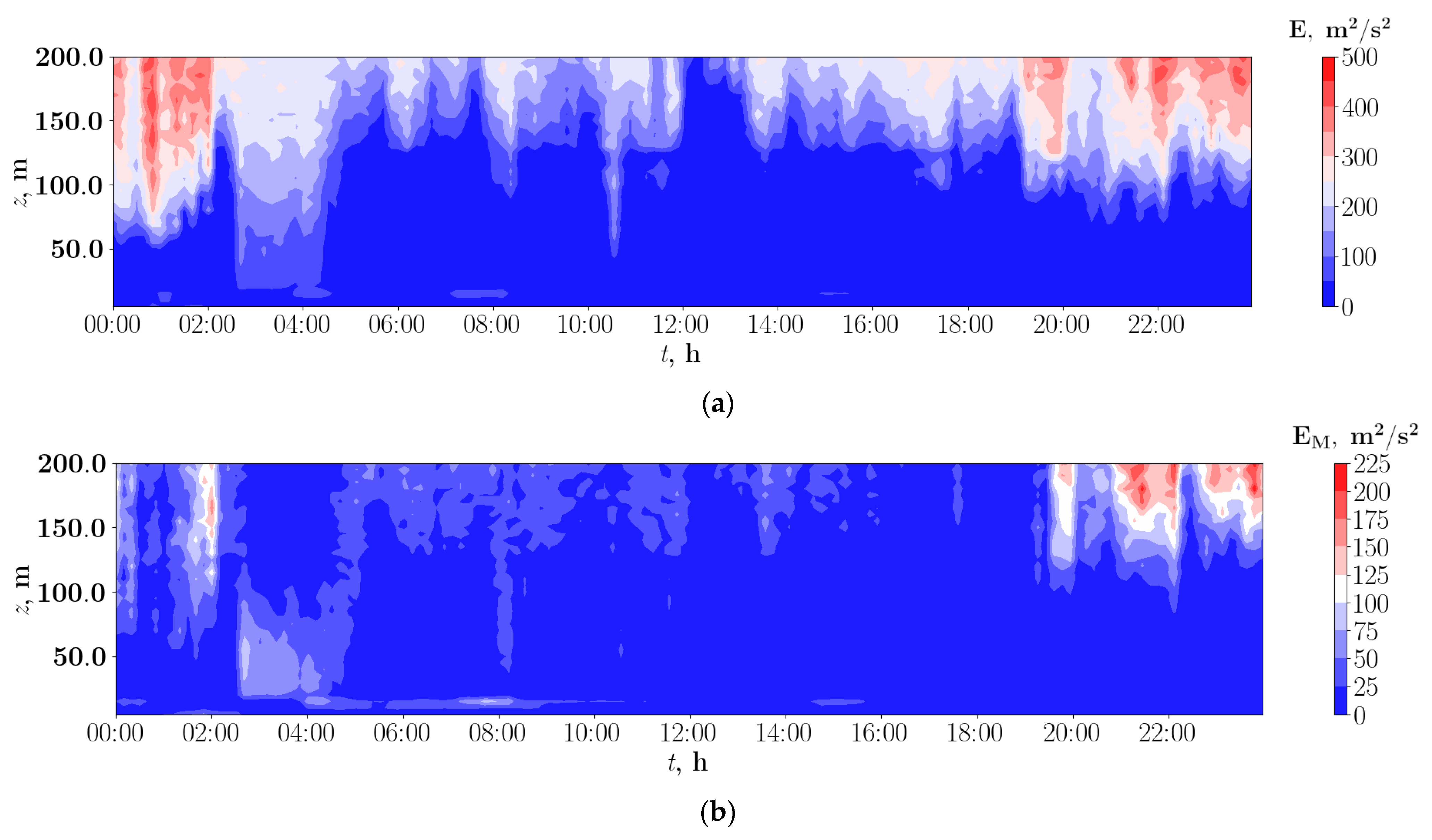
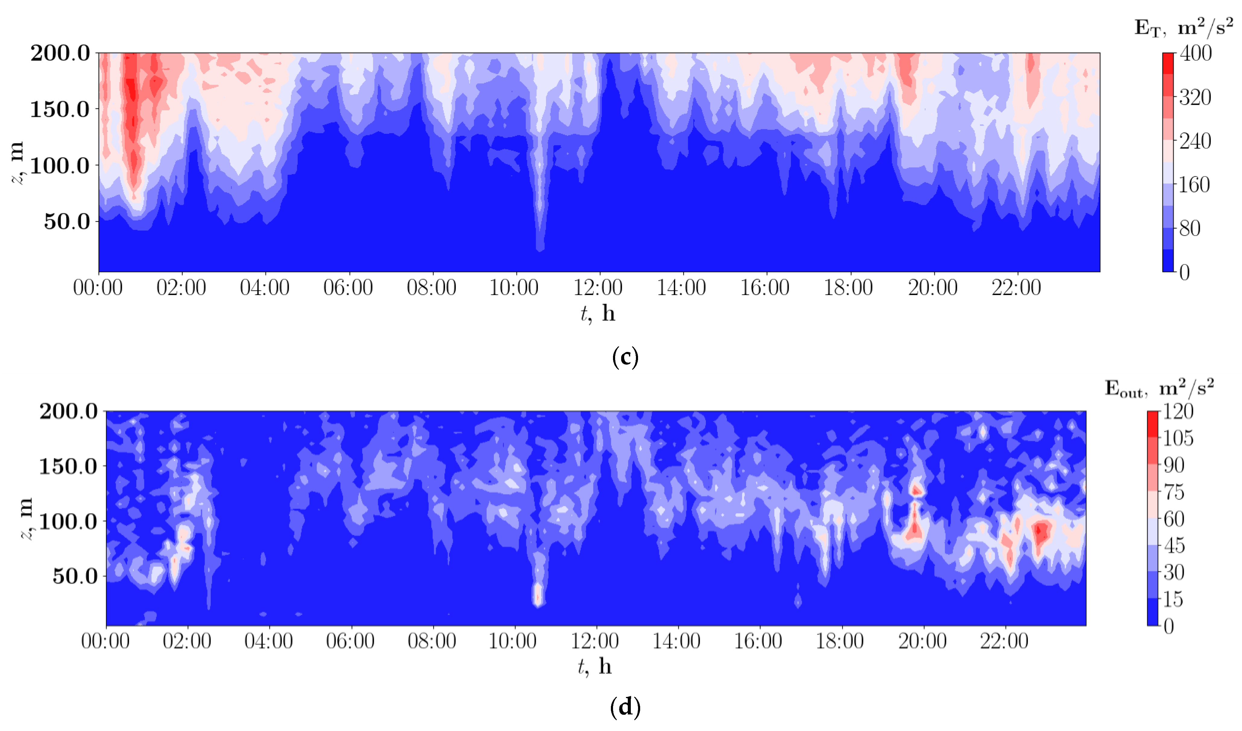
Figure 4 shows the diurnal hourly dynamics of the robust semi-nonparametric estimates of the total kinetic wind energy with an allowance for the outliers E (a); its mean, E_MKE (b), and turbulence, E_TKE (c), components; and the kinetic energy of the outliers $E_{\mathrm{out}}=E-E_0$ (d) retrieved by the postprocessing of the minisodar measurements. From Figure 4a, it can be seen that the maximum values (red color area) E_max ~ 500 m²/s² were observed at night, from 00:00 till 02:00, local time, and in the evening, from 19:00 till 24:00. However, whereas at night the lower boundary of the layer with enhanced kinetic energy was about 125 m, at night it descended to 75 m. From 02:00 till 19:00, E did not exceed 100 m²/s² in the lower layer. The upper boundary of this layer first ascended from about 50 m to 200 m at noon and then descended to 100 m.

The robust semi-nonparametric estimates of the diurnal hourly behavior of the mean kinetic wind energy component E_M (Figure 4b) demonstrated that from 04:00 till 19:00, its values were about 50 m²/s² and were practically independent of time of day and sensing altitude. From midnight till 02:30, E_M underwent local variations, and reached 225 m²/s² (red area) at altitudes above 125 m. From 02:30 till 04:00, it increased to 100 m²/s² at altitudes from 25 to 75 m (light blue area). From 19:00 till 24:00, areas with enhanced values of E_M ~ 225 m²/s² (red areas) were observed. As a whole, the contribution of E_M to the total kinetic wind energy E was low.

Figure 4c shows the robust semi-nonparametric estimates of the hourly dynamics each day of the turbulence kinetic energy component E_T obtained by the postprocessing of the minisodar measurements. From the figure, it can be seen that E_T increased with altitude z. In the lower layer, the altitude of which first increased from 75 m at 00:00 to 200 m at 01:00 and then decreased to 75 m at 24:00 undergoing significant altitude hourly variations, it did not exceed 80 m²/s². Above 75 m, an area of enhanced E_T was clearly visible.

Figure 4d shows the diurnal hourly dynamics of the kinetic wind energy of the outliers. It can be seen that the contribution of the outliers became especially pronounced at night from 00:00 till 02:00 at altitudes above 50 m. From 05:00 till 19:00, the kinetic energy of the outliers reached 60 m²/s² at altitudes above 100 m. In the evening and at night, the kinetic energy of the outliers (red areas) reached 120 m²/s², that is, providing significant contribution to the total kinetic energy E~200 m²/s² in this altitude range (see Figure 4a), and its effect was more pronounced at altitudes between 50 and 100 m.

6. Conclusions

Based on the proposed parametric, semiparametric, and semi-nonparametric algorithms developed by the authors, the spatiotemporal dynamics of the total kinetic wind energy without E₀, and with allowance E, for the kinetic energy of the outliers, E_out; its mean, E_M, and turbulence, E_T, components were analyzed by the postprocessing of the minisodar measurements of the three wind vector components and their variances in the lower 200 m layer of the atmosphere. The parametric, semiparametric, and semi-nonparametric robust algorithms for obtaining effective $\widehat{E}$, ${\widehat{E}}_0$, and ${\widehat{E}}_{\mathrm{out}}$ estimates with the model distributions $F(\mathsf{\zeta },\overrightarrow{\mathsf{\theta }}), G(\mathsf{\zeta },\overrightarrow{\mathsf{\theta }})$, and $H(\mathsf{\zeta },\overrightarrow{\mathsf{\theta }})$ used to analyze their spatiotemporal dynamics allowed us to reveal some important physical features. Without making allowances for the contribution of the kinetic energy of the outliers, the altitude profiles of the kinetic wind energy components in the ABL were depicted as quite smooth curves. The allowance for the contribution of the kinetic energy of the outliers revealed their thin-layered structure, thereby demonstrating the efficiency of the proposed robust algorithms. The nonmonotonic increase in the kinetic energy of the wind outliers with altitude sounding was established. Physically, this can be explained by the nonmonotonic increase in the turbulence kinetic energy of local air vortices in the ABL. The vertical extension of the outlier layers was of the order of 10–20 m.