A Fast Parallel Random Forest Algorithm Based on Spark

Abstract

To improve the computational efficiency and classification accuracy in the context of big data, an optimized parallel random forest algorithm is proposed based on the Spark computing framework. First, a new Gini coefficient is defined to reduce the impact of feature redundancy for higher classification accuracy. Next, to reduce the number of candidate split points and Gini coefficient calculations for continuous features, an approximate equal-frequency binning method is proposed to determine the optimal split points efficiently. Finally, based on Apache Spark computing framework, the forest sampling index (FSI) table is defined to speed up the parallel training process of decision trees and reduce data communication overhead. Experimental results show that the proposed algorithm improves the efficiency of constructing random forests while ensuring classification accuracy, and is superior to Spark-MLRF in terms of performance and scalability.

1. Introduction

Random forest (RF) is an ensemble learning algorithm that combines multiple decision trees to form a robust classifier [1]. Owing to the high prediction accuracy and good tolerance for outliers and noise in data, RF is widely used in various fields such as bioinformatics [2,3], classification [4,5,6,7], educational information [8], etc. Since all the decision trees are independent, RF algorithms are conducive to parallel implementation, making it one of the research hot spots in the current big data field. However, due to memory, time complexity, and data complexity limitations, traditional RF algorithms suffer from low accuracy and computational efficiency because of big data and feature redundancy [9]. Therefore, it is necessary to alleviate the influence of feature redundancy on classification accuracy and improve the computational efficiency of large-scale data.

In essence, RF is an integrated model composed of some decision trees including ID3 [10], C4.5 [11], CART algorithms, etc. Among them, the CART algorithm applies the binary tree construction and adopts the Gini coefficient to measure the impurity of variables. These features effectively simplify the scale of the decision tree and a large number of logarithmic operations and thus make the CART algorithm one of the popular ways for constructing decision trees. Yu et al. [12] introduced the confidence of instances and proposed a C_CART improvement algorithm, which improves the generalization performance and avoids over-fitting to some extent. Lin et al. [13] combined the multi-level logistic regression model with the CART algorithm, used binary results to model multi-level data, and improved the classification accuracy and specificity. Seere et al. [14] also proposed a hybrid learning model that combined the fuzzy minimum–maximum (FMM) neural network and CART algorithm. However, the traditional Gini coefficient definition needs to consider the influence of feature redundancy and might cause terrible classification performance because of serious feature redundancy. Therefore, a new Gini coefficient definition is proposed to alleviate the impact of feature redundancy on classification accuracy.

In addition, the Gini coefficient calculation relies on discrete data [15]. When the original data is continuous, it is necessary to discretize the original data by setting some candidate split points. On this basis, the traditional CART algorithm has to calculate the Gini coefficients of all candidate split points and select the one with the minimum Gini coefficient as the optimal split point. For a continuous feature with n values, there are n − 1 candidate split points for Gini coefficient calculation. As the amount of data increases, the number of candidate split points will significantly increase. The number of Gini coefficient calculations will also increase linearly and affect the efficiency of constructing decision trees. Therefore, reducing the number of candidate split points is necessary to improve the computational efficiency for large-scale data.

With the development of big data technology, the research on the random forest algorithm using parallel computing technology has become one of the current hot spots. Fernandes et al. [16] proposed an enhanced decision tree ranking algorithm to speed up distributed computing. Genuer et al. [17] parallelized and extended multiple variants of random forests for processing large-scale data and experimentally demonstrated the relative performance of different variants and their limitations. Sara et al. [18] partitioned imbalanced data using MapReduce and alleviated its impact on the algorithm. Mu et al. [19] introduced the Pearson correlation coefficient to determine the optimal split attribute and split point during decision tree growth and trained decision trees in parallel using MapReduce technology. Xu W et al. [20] calculated the information gain of various features on MapReduce computing framework by introducing a feature weighting system and improving existing data analysis with evaluation metrics. Chen et al. [21] combined data-parallel and task-parallel optimization methods to reduce communication costs between data and workload imbalances. Alessandro [22] grew all trees in parallel with a breadth-first node approach to reduce the number of data scans. In addition, Apache Spark Mlib [23] also provides a standard Spark-MLRF algorithm and is widely accepted by many researchers. In general, there are lots of iterations in a RF algorithm, and the output of the previous job is the input of the next job.

For the MapReduce computing framework, each job stores the intermediate results to disk during iterations, resulting in a large number of disk I/O operations and data storage requirements, leading to low running efficiency. Instead, the new generation big data technology Spark can cache data in memory and is more efficient in realizing the RF algorithm for large-scale data. However, in calculating the optimal split point of continuous features, the standard Spark-MLRF takes a random sampling strategy to achieve faster computation but a lower classification performance. In addition, when constructing a training subset, Spark-MLRF also provides each decision tree with a sampled data set consistent with the original data set size, resulting in a large storage load and data communication.

Aiming at the above existing problems, we propose an optimized parallel random forest algorithm based on Spark. The main contributions are as follows: (1) A new Gini coefficient definition is proposed to calculate the feature information and reduce the impact of feature redundancy on classification accuracy. (2) An approximate equal-frequency binning method is proposed to optimize the number of candidate split points of continuous features and effectively reduce the number of Gini coefficient calculations. (3) A parallel decision tree training method based on the forest sampling index (FSI) table is proposed. We achieve less storage load and data communication by establishing the index table for the entire random forest.

The rest of this paper is organized as follows. Section 2 briefly introduces the principle of the random forest algorithm and Spark technical framework. Section 3 improves the calculation of CART tree splitting information and proposes an approximate equal-frequency binning algorithm. Section 4 presents a parallel implementation of the proposed Random forest algorithm. Section 5 shows the related experimental results to evaluate the classification accuracy and parallel performance of the proposed algorithm. Section 6 concludes the work and presents an outlook for future research.

2. Preliminary Knowledge

2.1. Random Forest Algorithm

The random forest algorithm is an ensemble classification algorithm. First, it randomly extracts K different training subsets from the original data set to construct K decision trees. Next, all the decision trees are integrated into a random forest, and the final classification decision depends on the voting of decision trees.

Given a data set S with M features, the construction steps of Random forest are as follows:

Step 1, Data sampling. Randomly select K training subsets $\left\{S_1,S_2,\dots ,S_K\right\}$ of the same size as the original data set from the training data set S.

Step 2, Constructing decision trees. These decision trees are constructed recursively by C4.5 or CART algorithms from the corresponding training subset. For any subset $S_i$, m (m ≪ M) feature variables are randomly selected first. In the next process of node split, all the Gini coefficients of a feature are calculated to find the optimal split point. This split process is repeated until a leaf node is generated. Finally, K decision trees are trained in the same way from K training subsets.

Step 3, Voting decision. Combine K trained decision trees $\left\{h_1\left(S_1\right),h_2\left(S_2\right),\dots ,h_k\left(S_k\right)\right\}$ into a random forest model. The classification decision of RF model depends on voting among trees, and the most popular voting method is simple majority voting.

2.2. Apache Spark

Spark is an improved distributed computing framework based on MapReduce. The related research has shown that Spark’s computation speed is 100 times faster than MapReduce in large-scale data iterative operations [24]. With enough memory space, Spark can cache intermediate data and result in memory, significantly reducing the number of I/O operations between disks. Additionally, Spark avoids shuffle through local calculations and improves the efficiency of iterative calculations.

The core concept of Spark are the resilient distributed data sets (RDD), which implement application task scheduling, invocation, operation, and error recovery, and provide API for upper-layer components.

RDD is a lazy computing mechanism with two kinds of data operations. The first one is transformation, which creates a new RDD based on an existing RDD. The second is action, which triggers the calculation when executed and stores the RDD into the disk after obtaining a result. Some Spark API related to the algorithm in this paper is briefly introduced as follows. For a more comprehensive API function introduction, please refer to the official Spark documentation.

map(func): Convert each row of the original RDD to a new data structure through the map function to generate a new RDD.

mapPartitions(func): It is equivalent to map function, but the difference is that map performs a conversion operation on each row of RDD, and mapPartitions only performs a conversion operation on each data partition.

reduceByKey(func): Aggregate the data with the same key in RDD, so that the original key and the newly obtained value are combined to form a new row.

collect: Collect all elements in the data set as an array.

persist: Cache RDDs in memory.

3. Improved Random Forest Algorithm

In this section, we optimize the traditional random forest algorithm from two aspects including the following: (1) A new Gini coefficient is defined to reduce the impact of feature redundancy on classification accuracy. (2) An approximate equal-frequency binning method is proposed to optimize the number of candidate split points of continuous features and effectively reduce the number of Gini coefficient calculations.

3.1. The New Gini Coefficient

The Gini coefficient can measure the impurity of information and is usually applied by the CART algorithm to evaluate all split features. The smaller the Gini coefficient, the lower impurity and the stronger the correlation between the feature and the target. Suppose feature a has K different values, and the probability of kth sample value in the total samples is, then the Gini coefficient of feature a is defined as follows:

$$Gini\left(a\right)=\underset{k=1}{\sum ^K}{p}_k\left(1-p_k\right)=1-\underset{k=1}{\sum ^K}{p_k}^2$$

(1)

According to the above definition, the Gini coefficient of a data set D is described as follows, where $C_k$ represents the sample subset belonging to the kth class in the data set D, and K is the number of classes:

$$Gini\left(D\right)=1-\underset{k=1}{\sum ^K}{\left(\frac{\left|C_k\right|}{\left|D\right|}\right)}^2$$

(2)

If data set D is divided into two subset D₁ and D₂ by split point x of feature a, then the Gini coefficient of data set D with respect to feature a is defined as follows:

$$Gini\left(D,a\right)=\frac{\left|D_1\right|}{\left|D\right|}Gini\left(D_1\right)+\frac{\left|D_2\right|}{\left|D\right|}Gini\left(D_2\right)$$

(3)

where Gini(D) represents the uncertainty of data set D, and Gini(D, a) represents the new uncertainty if data set D is divided by split point x. The larger Gini coefficient, the greater the uncertainty of the data set.

Although the traditional CART algorithms consider the impact of conditional features on decision features, they analyze the redundancy between conditional features less. To avoid the impact of redundancy between features on classification accuracy, we define the conditional Gini coefficient based on the concept of conditional entropy.

Definition 1.

Given a data set D, the conditional Gini coefficient of feature a with respect to feature b is defined as follows:

$$Gini\left(a|b\right)=1-\underset{j=1}{\sum ^{num\_b}}\frac{\left|D_j\right|}{\left|D\right|}\underset{k=1}{\sum ^{num\_a}}{\left(\frac{{|D}_{jk}|}{\left|D_j\right|}\right)}^2$$

(4)

where num_b represents the number of categories of feature b, |D_j| is the number of samples that belong to the jth category of feature b, ${|D}_{jk}|$ is the number of samples in subset D_j that belong to the kth category of feature a, and num_a represents the number of categories of feature a in subset D_j. The smaller the Gini(a|b), the higher the redundancy between feature a and feature b.

Definition 2.

Given a feature set F = C − {a}, C represents all conditional features, then the average Gini coefficient of feature a with respect to feature set F is defined as follows:

$${Gini}_{aF}\left(D\right)=\frac{\sum _{f\in F}\left(Gini\left(a\right)-Gini\left(a\right|f)\right)}{\left|F\right|}.$$

(5)

where Gini(a|f) represents the conditional Gini coefficient under the known feature $f\in F$, and Gini(a) represents the Gini coefficient of feature a, the differences between feature a and other features are averaged to quantify the degree of correlation or redundancy on feature a.

When calculating the optimal split feature and split point, the feature redundancy information between feature a and other features should be subtracted to reduce the impact of feature redundancy on classification accuracy. To this end, a new Gini coefficient with low feature redundancy is defined as follows:

$$Gini\left(D,a,F\right)=\left[\frac{\left|D_1\right|}{\left|D\right|}Gini\left(D_1\right)+\frac{\left|D_2\right|}{\left|D\right|}Gini\left(D_2\right)\right]-{Gini}_{aF}\left(D\right).$$

(6)

Obviously, if the redundancy relationship between feature a and other features is small, then $Gini\left(D,a,F\right)$ is small, too. This means that feature a is highly likely to be selected as the split feature. A simple example is shown in

Table 1. Credit data example.

Age	Have a Job	Credit Status	Label
youth	no	generally	no
youth	no	good	no
youth	yes	good	yes
youth	yes	generally	yes
youth	no	generally	no
middle aged	no	generally	no
middle aged	no	good	no
middle aged	yes	good	yes
middle aged	no	very good	yes
middle aged	no	very good	yes
old age	no	very good	yes
old age	no	good	yes
old age	yes	good	yes
old age	yes	very good	yes
old age	no	generally	no

.

There are 15 samples in Table 1, which include 3 conditional features and 1 decision feature. Features a, b, and c represent “age”, “have a job”, and “credit status”, respectively. To simplify the next description, some digital marks are also adopted to represent the related feature values such as 1, 2, and 3 meaning youth, middle aged, and old age, respectively. The related values of “have a job” are represented by 1 and 2, which stand for yes and no, respectively. The values of “credit status” are represented by 1, 2, and 3, which stand for very good, good, and generally, respectively.

For the traditional calculation method, the Gini coefficient of feature a is calculated by formula (3); it has $Gini\left(D,a=1\right)=0.44,Gini\left(D,a=2\right)=0.48,Gini\left(D,a=3\right)=0.44$. The Gini coefficient of feature b is as follows: $Gini\left(D,b=1\right)=0.32$. The Gini coefficient of feature c is as follows: $Gini\left(D,c=1\right)=0.36,Gini\left(D,c=2\right)=0.47,Gini\left(D,c=3\right)=0.32$. Since $Gini\left(D,b=1\right)$ and $Gini\left(D,c=3\right)$ are the smallest coefficients, both feature b and c are thus considered as the best split features, and b=1 and c=3 are the best split points, respectively.

According to formula (1), $Gini\left(b\right)=0.44$, $Gini\left(c\right)=0.658$. According to formula (4), $Gini\left(b|a\right)=0.427,Gini\left(b|c\right)=0.407$, it has ${Gini}_{bF}\left(D\right)$=0.023. At the same time, $Gini\left(c|a\right)=0.587,Gini\left(c|b\right)=0.627$, it has ${Gini}_{cF}\left(D\right)$ = 0.051. According to formula (6), $Gini\left(D,b=1,F\right)=0.32-0.023=0.297,Gini\left(D,c=3,F\right)=0.32-0.051=0.269$. Finally, feature c is chosen as the best split feature, and c=3 is the optimal split point. Obviously, feature c has lower redundancy compared to other features.

3.2. Approximate Equal-Frequency Binning Method

For a continuous data set, the traditional random forest algorithms have to discretize the continuous value and average all adjacent feature values to set candidate split points. Assuming that a continuous feature a has m different sample values, arranged from small to large $a_1,a_2,\dots ,a_m$, the traditional CART algorithm has to calculate the average of adjacent two sample values to obtain m − 1 candidate split points, where the ith candidate split point $T_i$ is expressed as $T_i=\left(a_i+a_{i+1}\right)/2$. This means that it has to calculate m − 1 Gini coefficients for feature a to find out the optimal split point. Obviously, when dealing with massive data, these candidate split points will cause lots of Gini coefficient calculations and reduce the efficiency of operation.

To reduce the number of candidate split points, improve training efficiency, and ensure that classification accuracy is not significantly reduced, we propose an approximate equal-frequency binning method to optimize the number of candidate split points.

The approximate equal-frequency binning method places the values of continuous features into different bins and continuously takes the average of the maximum value in the previous bin and the minimum value in the next bin to obtain all candidate split points. This method mainly includes two steps. In the first step, the feature values are sorted in ascending order, and the number of occurrences of each value is counted. Additionally, the total number of bins is usually set to the square root of the number of different values. In the second step, the feature values are classified into different bins one by one, and the boundaries between each bin are calculated to obtain all candidate split points. Algorithm 1 provides the specific steps of the approximate equal-frequency binning method.

Algorithm 1: Approximate equal frequency binning algorithm

Input: Continuous values of feature a $\left\{a_1,a_2,\dots ,a_{n-1},a_n\right\}$

Output: All candidate split points of feature a

Step 1: All feature values are sorted in ascending order; Step 2: Obtain all distinct values ${\mathrm{A}}^{\prime }=\left\{{a^{\prime }}_1,{a^{\prime }}_2,\dots ,{a^{\prime }}_{m-1},{a^{\prime }}_m\right\}$ and the number of each value counts = {count1, count2, …, countm}; Step 3: Set the number of boxes bins = int(sqrt(num(A′))); Step 4: The size of the current bin is set to a constant S = sum(counts)/bins; Step 5: The binning operation. All feature values are processed sequentially;

Step 5.1 If counti >= S then a′i is treated as a large number and boxed individually, set the average of this feature value and the next feature value as the candidate split point;

Step 5.2 If counti < S then add the remaining feature value in order until the number of feature value is greater than or equal to S. At this time, the average of the largest feature value in the box and the next feature value not in the box is set as the candidate split point;      Step 5.3 bins = bins − 1; if bins = 1, go to step 6, or jump to step 4. Step 6: Put all remaining feature value into the last bin and the algorithm ends.

A simple example is described in Figure 1 to show the process of Algorithm 1. Assuming a feature with the value set [1,1,1,2,1,3,4,8,1,4,5,6,1,7,9], the proposed approximate equal-frequency binning algorithm sorts the feature values and obtains A′ = [1,2,3,4,5,6,7,8,9], counts = {6,1,1,2,1,1,1,1,1}. At this time, bins are set to 3, which means the average size S of a bin is 5. Since the count of “1” is 6, all the values of “1” are put into the same bin as [1,1,1,1,1,1] and the related split point is 1.5. Next, jump to Step 4 and recalculate S as 4.5, then the next bin includes five numbers as [2,3,4,4,5], and the related split point is 5.5. Finally, the last bin [6,7,8,9] is obtained in Step 6. In conclusion, there are only two candidate split points and the related Gini coefficients are calculated twice. In contrast, the traditional random forest algorithm has to generate eight candidate split points. It means that the Gini coefficients on this feature have to be calculated eight times. Obviously, Algorithm 1 can effectively improve computational efficiency, and the larger the data set, the more obvious the superiority is.

4. Parallelization of Random Forest Based on Spark

To improve the computing performance for big data sets, we propose two optimization strategies based on Spark including the following: (1) Parallel decision tree training strategy based on a forest sampling index table (FSI). The FSI table is defined to record the indexes of all training subsets. Based on FSI and the related RDD partitioned data, all the decision trees are trained in a parallel model, which effectively reduces the demand for data transmission in a distributed environment. (2) Gini coefficient calculation optimization strategy based on dictionary. When searching for the best split point of a certain feature, two dictionaries are declared to reduce the number of traversals from the traditional (n − 1) times to once, which effectively improves the calculation speed of the split point and avoids repeated traversal of the entire data set.

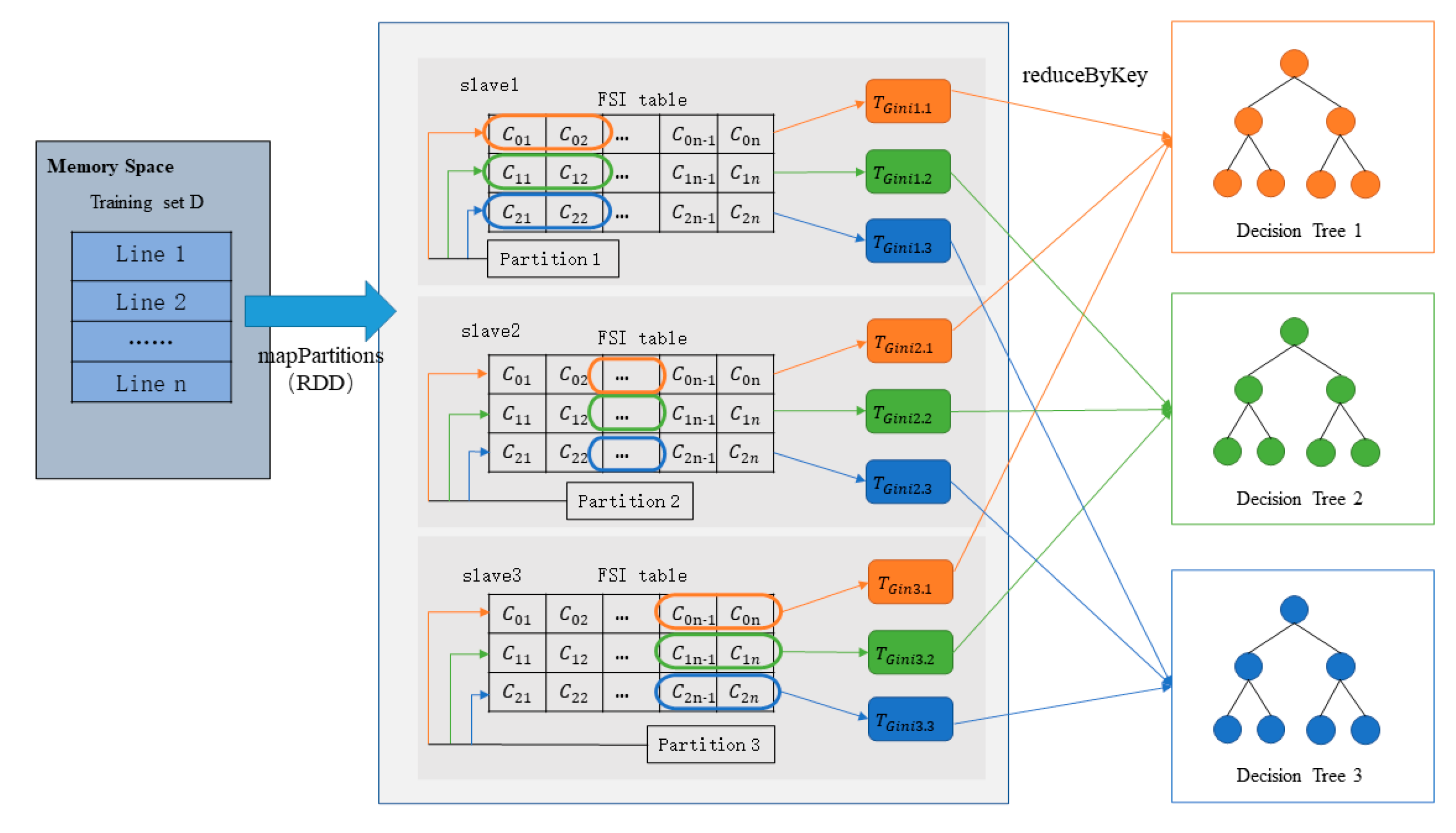
4.1. Parallel Decision Tree Training Strategy Based on a Forest Sampling Index Table

In the traditional random forest algorithm, it is necessary to obtain a training subset for each decision tree through the random sampling method (bagging) and construct a decision tree based on each training subset. The training process is shown in Figure 2.

Usually, the size of the training subset is proportional to the size of the original data set. Therefore, when the original data set is large, Spark has to allocate extra space to store the sampled training subset, which causes a large number of disk I/O operations and less computational efficiency. To address this issue, we define a forest sample index table (FSI) to record the indexes of all training subsets to reduce the storage requirement. The detailed definition is as follows.

Definition 3.

Given a data set D, the forest sampling index table FSI on k training subsets is defined as follows:

$$\mathit{FSI}=\left[\begin{array}{c}\begin{array}{c}{C}_{01},C_{02},\dots ,C_{0n}\\ C_{11},C_{12},\dots ,C_{1n}\\ \dots \end{array}\\ C_{\left(k-1\right)1},C_{(k-1)2},\dots ,C_{(k-1)n}\end{array}\right]$$

FSI is a k × n binary matrix. Each row represents the index of a training subset, which can be used to train a decision tree. $C_{ij}$ represents the sampling situation of sample j with respect to ith training subset. If $C_{ij}$ is 1, it means that the ith subset contains sample j, otherwise sample j does not participate in the construction process of the ith decision tree.

The FSI table records the indexes of all the k subsets and is allocated to each slave node. During the training process of each decision tree, the related data is loaded from the RDD data partitions according to the FSI table, and the related Gini coefficient is calculated directly in memory. That is, it does not store the training subset repeatedly.

The detailed parallel decision tree training process based on the FSI table is shown in Figure 3. First, the FSI table is allocated to all slave nodes. At the same time, the original data set is divided into k RDD data partitions by mapPartition function, and each RDD data partitions is allocated to the corresponding slave nodes to achieve data parallel processing, namely Partition_1, Partition_2, … , and Partition_k, respectively. Next, each slave node processes the corresponding RDD data partition based on the FSI table and calculates the Gini coefficients of the related candidate splitting points. Each Gini coefficient calculation task $T_{Gini}$ loads data records from the RDD partition according to the indexes in the FSI table. Finally, the candidate splitting points of all slave nodes are compared by reduceByKey function to find out the optimal one for a decision tree.

For example, tasks $T_{Gini1.1}$,$T_{Gini1.2}$ and $T_{Gini1.3}$ on slave1 calculate the Gini coefficients of decision trees 1, 2, and 3, respectively, and find out the local best split point. Next, these parallel outputs of $T_{Gini}$ are combined by reduceByKey function to find out the best global split point. In detail, tasks $\left\{T_{Gini1.1},T_{Gini\mathrm{1,2}},T_{Gini1.3}\right\}$ are used to construct decision tree 1, tasks $\left\{T_{Gini2.1},T_{Gini\mathrm{2,2}},T_{Gini2.3}\right\}$ are used to construct decision tree 2, and tasks $\left\{T_{Gini3.1},T_{Gini\mathrm{3,2}},T_{Gini3.3}\right\}$ are used to construct decision tree 3.

4.2. Gini Coefficient Calculation Optimization

According to formula (3), the Gini coefficient of each candidate split point depends on two subsets D₁, D₂, and their class distribution. This means that the traditional random forest algorithm has to traverse the entire data set when dealing with continuous features. If there were n − 1 candidate split points for a certain feature, then it is necessary to traverse (n − 1) training subsets. Obviously, the computational efficiency is low for a big data set.

In this paper, we declare two dictionaries named left and right to optimize the Gini coefficient calculation. The dictionary is expressed as {key1:value1, key2:value2, …, key n:value n}, where key is the feature value category, and value is the number of categories. Left and right are used to store the information of each category in the left and right subsets after splitting, respectively.

At the initial state, left is an empty dictionary, and right contains all categories and their corresponding number of occurrences in the local data set. Next, for each candidate split point, the feature value smaller than the split point is divided into the left subset, and the other feature values still remain in the right subset. On this basis, the additional category and numbers in the left subset are accumulated into the left dictionary, and are subtracted from the right dictionary. At this time, the left and right, respectively, represent the category distribution of the left and right subsets. The Gini coefficient of this candidate split point can be directly calculated based on the left and right dictionaries. In detail, value_k represents |$C_k|$, which means the number of kth sample categories. The sum of all value in the left dictionary means |D₁|, and the sum of all value in the right dictionary represents |D₂|. Therefore, the related Gini coefficient can be easily calculated based on the two dictionaries, and it is unnecessary to traverse the entire data set. A simple example is given here to illustrate this optimization process.

Table 2. A simple data set.

Feature Value	Category
0.1	1
0.3	2
0.7	1
0.7	1
1.2	3

shows a feature column and its corresponding categories. Initialize left = {} and traverse the entire data set to obtain right = {1:3, 2:1, 3:1}. For the first candidate split point 0.2, the states of two dictionaries are altered as left = {1:1} and right = {1:2, 2:1, 3:1}. At this point, the number of samples in the left subset is |D₁| = 1, and the number of samples in the right subset is the sum of value of right dictionary |D₂| = 4. In addition, the number of sample categories in the left subset is ${|C}_1|=1$, and the number of sample categories in the right subset is ${|C}_1|=2$, ${|C}_2|=1$,$\left|C_3\right|=1$. According to formula (3), the Gini coefficient of this candidate split point is 0.45. Similarly, for the second split point 0.5, the states of two dictionaries are updated to left = {1:1, 2:1} and right = {1:2, 3:1}, |D₁| = 2, |D₂| = 3, |$C_1|=1,|C_2|=1$ in the left subset, and ${|C}_1|=2,|C_3|=1$ in the right subset, then the Gini coefficient is 0.53. Repeat the above process until the Gini coefficients of all candidate points are calculated. Obviously, the new Gini coefficient calculation method only traverses the original data set once in the initialization process. In contrast, the traditional method requires to traverse data set n − 1 times.

4.3. Parallel Implementation of Improved Random Forest Algorithm

Figure 4 shows the overall structure of the proposed optimized random forest algorithm, and the parallel implementation process of the random forest is described in Algorithm 2.

Algorithm 2: Parallel Training Process of Optimization Random Forest

Input: The number of decision trees K, data set D, the FSI table

Output: Random forest model 1: For i = 0 to (K − 1) 2:    For index in range(start, end) 3:      For j, feature in enumerate(featureIndex) 4:         Sc.broadcast(FSI)//Build an index table and load the training subset 5:          Left = {},right = {}//Declare two dictionaries to record the number of labels for the two subsets

6:          LeftLen = 0,rightLen=len(node.recoeds)//Number of categories for the left and right subsets 7:          The set of candidate split points is obtained based on Algorithm 1 8:          For thisSplitVal in spiltNode 9:              Divide the left and right subsets according to the split point 10:                LeftLen + = 1,rightLen − = 1

11:              Calculate the Gini coefficient according to Equation (6) 12:              Take the split point with the smallest Gini coefficient 13:          End for 14:      End for 15:      Obtain the best split feature and the best split spot, split the current node according to these two values, generate two new child nodes, and continue splitting until all nodes are leaf nodes 16:    End for 17:    Training to obtain a single decision tree 18: End for

The time complexity of the traditional random forest algorithm is $O\left(KMN\log N\right)$, where K is the number of decision trees in the random forest algorithm, M is the number of features, N is the number of samples, and $\log N$ is the average depth of all tree models.

For Algorithm 2, the time complexity of the approximate equal-frequency binning method described in Section 3.2 is $O\left(MN\right)$. At this time, the size of data set is reduced from N to n, where n is the number of bins and less than sqrt(N). Therefore, the time complexity of training a base classifier is $O\left(MN+Mn\log N\right)$ and the total time complexity of the entire algorithm is $O\left(K\left(MN+Mn\log N\right)\right)$. When implementing an optimized random forest algorithm based on Spark, K trees are constructed in parallel. Therefore, the parallelized time complexity is $O\left(K\left(MN+Mn\log N\right)/KM\right)=O\left(N+n\log N\right).$ In the big data environment, the number of samples N is very large; it is thus efficient to reduce N to n to improve the algorithm’s performance.

5. Experiments

To evaluate the performance of the proposed algorithm, we conducted several comparative experiments. Section 5.2 presents a comparison of single machine performance, which was conducted on a machine with a CPU frequency of 2.9 GHz, 16 GB of memory, and a 64-bit operating system. Section 5.3 presents distributed environment performance, which was carried out on the supercomputer of the High Performance Computing Platform at Central South University. The related experiments were performed on a cluster with 48 cores, each of which has an Intel Xeon Gold 6248R core model, 3.0 GHz main frequency, and 192 GB RAM memory. The software and their versions used in the experimental process were Spark 2.3.1, Hadoop 2.7.3, JDK 1.8.0, Scala 2.12.6, and Python 3.7.4.

5.1. Data Set Description

There are 11 data sets with different scales selected from the UCI machine learning library [25], including 7 small and 4 large data sets. The specific information of each data set is shown in

Table 3. Data set information.

Data Set	Instances	Features	Class
Glass	214	9	7
Wine	178	13	3
Ionosphere	351	33	2
Optical	3823	64	10
Image	2310	19	7
Letter	20,000	16	26
Adult	48,842	14	2
HT_senor	919,438	11	100
WinniPeg	325,834	175	7
Swarm	24,017	2400	2
SUSY	5,000,000	18	2

.

5.2. Evaluation of Algorithm Performance

Four evaluation indicators, Accuracy, Precision, Recall, and F1-value, are used to measure the classification performance of the algorithm. The calculation formula of the evaluation indicators is as follows:

$$Accurcacy=\frac{TP+TN}{TP+TN+FP+FN}$$

(7)

$$Precision=\frac{TP}{TP+FP}$$

(8)

$$Recall=\frac{TP}{TP+FN}$$

(9)

$$F1=\frac{2}{1/Precision+1/Recall}$$

(10)

where TP and FN are the numbers of correctly and incorrectly classified compounds of the actual positive class, respectively. Similarly, TN and FP denote the number of correctly and incorrectly classified compounds of the actual negative class.

This section used seven small data sets from UCI, Glass, Wine, Letter, Ionosphere, Optical, Image, and Adult to compare the accuracy and running time with RF and MGARF [26]. All data were divided into 70% for training and 30% for testing, and the number of trees was set to 200. The selection rate of the best individual and the seed selection rate parameters of MGARF was set to 0.8, and other parameters were set to their default values according to the literature [26]. The experimental results are shown in

Table 4. Accuracy and runtime comparison.

	Our Algorithm		RF		MGARF
Data Set	Acc	Time (s)	Acc	Time (s)	Acc	Time (s)
Wine	0.9815	3.7	0.9455	3.8	0.9735	68.8
Glass	0.7538	4.4	0.7425	4.1	0.7325	73
Image	0.9547	4.7	0.9018	3.9	0.9679	34.3
Ionosphere	0.9057	8.3	0.9146	9.5	0.8928	25.3
Letter	0.9532	43.2	0.9321	46.4	0.9482	477.6
Optical	0.9564	51.9	0.9608	30.6	0.9652	98.2
Adult	0.8688	167.2	0.8512	173.8	0.8466	358.9

The best performance is shown in bold.

.

The best performance is shown in bold.As shown in Table 4, the algorithm proposed in this paper has achieved the best classification results on the four data sets of Wine, Glass, Letter, and Adult. Furthermore, compared with the traditional Random Forest (RF) algorithm, the proposed algorithm achieved an average 2.01% higher classification accuracy, indicating that the classification accuracy is improved by correcting the redundant relationships among features. Additionally, the run time of the proposed algorithm is relatively faster than that of the MGARF algorithm, which indicates that the approximate equal-frequency binning method reduces the number of candidate split points and sacrifices a certain degree of accuracy in exchange for improved efficiency.

These running times on small to medium data sets are shown in Figure 5. Our algorithm has slightly longer running times for some small data sets compared to RF because of the new Gini coefficient definition. However, as the size of the data set increases, the advantage of the proposed algorithm in terms of running time becomes apparent. For some medium data sets, such as Ionosphere, Letter, and Adult, the proposed algorithm has fewer running times and a 5.03% reduction in average running time compared to RF. Furthermore, the traditional random forest algorithm based on single machine computation is difficult to handle large-scale data within an acceptable time range. It tends to experience memory overflow during the execution, resulting in program termination. Instead, the proposed algorithm is effective for parallel computing in a distributed environment.

In addition, the algorithm in this paper is also compared with the current popular classification algorithms K-nearest neighbor (KNN), support vector machines (SVM) [27], and naïve bayes (NB) [28]. In the experiment, these three classification algorithms are implemented using the sklearn machine learning library, and the parameters of these algorithms are set to default values. The four indicators of Accuracy, Precision, Recall, and F1-value are mainly compared and analyzed. The experimental results are five-fold cross-validation. For the repeatability of the experiment, the random seed random_state is set to a fixed value of 42 in the algorithm, and the experimental results are shown in

Table 5. Comparison results of different algorithms.

Data Set		Our Algorithm	KNN	SVM	NB
Wine	Accuracy	0.9815	0.7782	0.9255	0.9818
	Precision	0.9833	0.7933	0.9433	0.9867
	Recall	0.9825	0.7611	0.9278	0.9867
	F1-value	0.9824	0.7602	0.9245	0.9852
Glass	Accuracy	0.7538	0.6705	0.6000	0.5692
	Precision	0.8559	0.5316	0.5279	0.4306
	Recall	0.6846	0.5601	0.5509	0.4980
	F1-value	0.7058	0.5296	0.5200	0.4482
Image	Accuracy	0.9547	0.9079	0.9460	0.7984
	Precision	0.9563	0.9123	0.9510	0.8378
	Recall	0.9543	0.9134	0.9489	0.8126
	F1-value	0.9533	0.9105	0.9483	0.7982
Ionosphere	Accuracy	0.9057	0.8784	0.8403	0.8221
	Precision	0.9095	0.9247	0.8936	0.8224
	Recall	0.8642	0.8357	0.7870	0.8385
	F1-value	0.8769	0.8482	0.8022	0.8171
Letter	Accuracy	0.9532	0.9017	0.8352	0.6437
	Precision	0.9542	0.9053	0.8367	0.6562
	Recall	0.9531	0.8997	0.8331	0.6423
	F1-value	0.9532	0.9004	0.8327	0.6390
Optical	Accuracy	0.9564	0.9538	0.9695	0.8204
	Precision	0.9569	0.9552	0.9713	0.8613
	Recall	0.9564	0.9519	0.9688	0.8174
	F1-value	0.9564	0.9527	0.9691	0.8167
Adult	Accuracy	0.8688	0.7749	0.7828	0.7983
	Precision	0.8207	0.6811	0.8795	0.7419
	Recall	0.7792	0.6032	0.5457	0.6297
	F1-value	0.7962	0.6154	0.5216	0.6494
Average	Accuracy	0.9106	0.8379	0.8738	0.7672
	Precision	0.9195	0.8148	0.8576	0.7624
	Recall	0.8820	0.7893	0.8953	0.7465
	F1-value	0.8892	0.7881	0.7883	0.7363

The best performance is shown in bold.

.

It can be seen from Table 5 that other classification algorithms are only better than the algorithm in this paper in some indicators, and only the SVM algorithm is better than the algorithm in this paper in calculating the average of the classification indicators of all test data sets. Therefore, compared with other classification algorithms, the proposed algorithm has a better classification performance.

In order to conduct statistical analysis on the test results, this paper uses the Friedman test [29] to verify whether there is a significant difference between the methods, where the null-hypothesis of Friedman test is that the tested indices are equivalent. There are seven data sets and six classifiers, the Friedman statistics F_F are distributed according to the F-distribution with 5 and 30 degrees of freedom, and the significance level for the critical value of α = 0.05 is 2.534. According to the average rank of the Accuracy indicators in Table 4 and Table 5, the F_F statistic is 5.321, which is greater than 2.534. Therefore, we reject the null hypothesis that there is a significant difference between the classification algorithms. Therefore, we use the Nemenyi post hoc test [29] to evaluate the pairwise differences, where the critical difference (CD) is 2.850 for α = 0.05. Figure 6 depicts the average rank of each classification algorithm for the Nemenyi post hoc test on the Accuracy evaluation indicators. When the pairwise difference of the two algorithms is greater than the CD, it indicates that there is a significant difference between the two algorithms. It can be seen from Figure 6 that the classification performance of the algorithm proposed in this paper is significantly higher than NB and KNN classification algorithms because the approximate equal-frequency method proposed in this paper sacrifices some classification performance in exchange for the computational efficiency of the algorithm; thus, compared with RF, MGRAF algorithm in this paper the classification effect is not significant.

5.3. Parallel Performance Evaluation

In this section, we use speedup, scaleup, and sizeup [30] to evaluate the parallel performance of the proposed algorithm and compare it with the standard Spark-MLRF algorithm.

5.3.1. Speedup

The Speedup evaluation method keeps the amount of data constant and increases the number of physical cores in the cluster to m times to measure the acceleration capability of an algorithm as the cluster resources increase. The calculation formula is as follows:

$$\mathrm{s}\mathrm{p}\mathrm{e}\mathrm{e}\mathrm{d}\mathrm{u}\mathrm{p}\left(m\right)=\frac{\mathrm{r}\mathrm{u}\mathrm{n} \mathrm{t}\mathrm{i}\mathrm{m}\mathrm{e} \mathrm{o}\mathrm{n} \mathrm{a} \mathrm{s}\mathrm{i}\mathrm{n}\mathrm{g}\mathrm{l}\mathrm{e} \mathrm{c}\mathrm{o}\mathrm{m}\mathrm{p}\mathrm{u}\mathrm{t}\mathrm{e}\mathrm{r}}{\mathrm{r}\mathrm{u}\mathrm{n} \mathrm{t}\mathrm{i}\mathrm{m}\mathrm{e} \mathrm{o}\mathrm{n} m \mathrm{c}\mathrm{o}\mathrm{m}\mathrm{p}\mathrm{u}\mathrm{t}\mathrm{e}\mathrm{r}\mathrm{s}}$$

(11)

If the speedup (m) can maintain a linear growth with the increase in m, then the parallelization performance of the algorithm is excellent for reducing the computation time. However, it is difficult to achieve linear speedup due to the additional time consumption caused by unbalanced data transmission and task assignment. In this section, the speedup values were tested when launching 1, 8, 16, and 32 computing cores on the HT_sensor, Winnipeg, Swarm, and SUSY data sets, respectively, and compared with Spark-MLRF. The experimental results are shown in Figure 6.

As shown in Figure 7, the algorithm has a relatively stable acceleration process with the increase in the number of cores, and the speedup growth of the proposed algorithm is closer to linear growth than that of Spark-MLRF.

5.3.2. Scaleup

The Scaleup evaluation method expands the amount of data to m times and increases the number of machines to m times at the same time. The calculation formula is as follows:

$$\mathrm{s}\mathrm{c}\mathrm{a}\mathrm{l}\mathrm{e}\mathrm{u}\mathrm{p}\left(DB, m\right)=\frac{\mathrm{r}\mathrm{u}\mathrm{n} \mathrm{t}\mathrm{i}\mathrm{m}\mathrm{e} \mathrm{f}\mathrm{o}\mathrm{r} \mathrm{p}\mathrm{r}\mathrm{o}\mathrm{c}\mathrm{e}\mathrm{s}\mathrm{s}\mathrm{i}\mathrm{n}\mathrm{g} DB \mathrm{o}\mathrm{n} \mathrm{a} \mathrm{s}\mathrm{i}\mathrm{n}\mathrm{g}\mathrm{e}\mathrm{l} \mathrm{c}\mathrm{o}\mathrm{m}\mathrm{p}\mathrm{u}\mathrm{t}\mathrm{e}\mathrm{r}}{\mathrm{r}\mathrm{u}\mathrm{n} \mathrm{t}\mathrm{i}\mathrm{m}\mathrm{e} \mathrm{f}\mathrm{o}\mathrm{r} \mathrm{p}\mathrm{r}\mathrm{o}\mathrm{c}\mathrm{e}\mathrm{s}\mathrm{s}\mathrm{i}\mathrm{n}\mathrm{g} m\times DB \mathrm{o}\mathrm{n} m \mathrm{c}\mathrm{o}\mathrm{m}\mathrm{p}\mathrm{u}\mathrm{t}\mathrm{e}\mathrm{r}\mathrm{s}}$$

(12)

If the scaleup (DB, m) can stay around 1.0 as the value of m changes, then the algorithm can adapt well to the changes in the size of the data set in a distributed environment. In this experiment, HT_sensor, Winnipeg, Swarm, and SUSY were selected as the experimental data sets to test the change of scaleup and compare with Spark-MLRF. Three different methods were used to test the change in the value of scaleup on each data set. (1) Start 8 computing cores to calculate a quarter subset of the data set. (2) Start 16 computing cores to calculate a half subset of the data set. (3) Start 32 computing cores to calculate the complete data set. The experimental results are shown in Figure 7.

According to reference [31], good performance can be achieved when the scaleup is greater than 0.5. As shown in Figure 8, with the increase in the number of cores and data volume, the scaleup of the proposed algorithm is above 0.6, and the decrease rate is relatively flat compared to Spark-MLRF. When the number of cores increases to 32, the scaleup of our algorithm is more than Spark-MLRF—on average, 7.45% higher. This result indicates that the algorithm proposed in this paper has better adaptability to changes in the size of parallel data sets.

5.3.3. Sizeup

The Sizeup evaluation method increases the amount of data to test the time complexity of the algorithm while keeping the number of cluster cores constant. The calculation formula is as follows:

$$\mathrm{s}\mathrm{i}\mathrm{z}\mathrm{e}\mathrm{u}\mathrm{p}\left(DB, m\right)=\frac{\mathrm{r}\mathrm{u}\mathrm{n} \mathrm{t}\mathrm{i}\mathrm{m}\mathrm{e} \mathrm{o}\mathrm{n} m\times DB}{\mathrm{r}\mathrm{u}\mathrm{n} \mathrm{t}\mathrm{i}\mathrm{m}\mathrm{e} \mathrm{o}\mathrm{n} \mathrm{t}\mathrm{h}\mathrm{e} DB}$$

(13)

In this experiment, we choose the SUSY data set, set the number of cores to 32, control the number of attributes to 18, and test the Sizeup values when the number of samples is 1,000,000, 2,000,000, 3,000,000, and 4,000,000. The experimental results are shown in Figure 9.

As shown in Figure 9, the growth rate of the algorithm’s running time is significantly lower than the growth rate of the data volume. The acceleration effect shown in Figure 8 orientates from the proposed approximate equal-frequency binning algorithm, which reduces the sample traversal number from N to n, reducing the computational process and effectively improving the operating efficiency of the algorithm.

6. Conclusions

In this paper, we propose a fast parallel random forest algorithm for big data. In theory, we introduce a new definition of the Gini coefficient to reduce the impact of redundancy between features. Additionally, we propose an approximate equal-frequency binning method to reduce the number of candidate split points for continuous features, thereby improving computation speed for searching the optimal split point. During the engineering implementation on Apache Spark platform, we defined a forest sampling index table to reduce data storage requirements and two dictionaries to greatly reduce the number of data traversals. The experimental results show that our algorithm outperforms the standard Spark-MLRF algorithm in key indicators such as speedup, scaleup, and sizeup, demonstrating good parallel performance and scalability.

The approximate equal-frequency binning method proposed in this paper may lose some split points that are good for the classification of the algorithm, resulting in a de-crease in classification accuracy. In addition, we use balanced data sets in the experiments and do not consider the impact of unbalanced data sets on the classification effect of the algorithm. Therefore, in the future, we can study the performance optimization of the algorithm on the unbalanced data set and how to screen out the segmentation points with better classification effects to improve the classification accuracy.

References

1. Breiman, L. Random forests. Mach. Learn. 2001, 45, 5–32. [Google Scholar] [CrossRef]
2. Dziak, J.J.; Coffman, D.L.; Lanza, S.T.; Li, R.; Jermiin, L.S. Sensitivity and specificity of information criteria. Brief. Bioinform. 2020, 21, 553–565. [Google Scholar] [CrossRef] [PubMed]
3. Ali, M.A.S.; Orban, R.; Rajammal Ramasamy, R. A Novel Method for Survival Prediction of Hepatocellular Carcinoma Using Feature-Selection Techniques. Appl. Sci. 2022, 12, 6427. [Google Scholar] [CrossRef]
4. Phan, T.N.; Kuch, V.; Lehnert, L.W. Land Cover Classification using Google Earth Engine and Random Forest Classifier—The Role of Image Composition. Remote Sens. 2020, 12, 2411. [Google Scholar] [CrossRef]
5. Zheng, X.; Jia, J.; Chen, J.; Guo, S.; Sun, L.; Zhou, C.; Wang, Y. Hyperspectral Image Classification with Imbalanced Data Based on Semi-Supervised Learning. Appl. Sci. 2022, 12, 3943. [Google Scholar] [CrossRef]
6. Khan, S.N.; Li, D.; Maimaitijiang, M. A Geographically Weighted Random Forest Approach to Predict Corn Yield in the US Corn Belt. Remote Sens. 2022, 14, 2843. [Google Scholar] [CrossRef]
7. Memiş, S.; Enginoğlu, S.; Erkan, U. Fuzzy parameterized fuzzy soft k-nearest neighbor classifier. Neurocomputing 2022, 500, 351–378. [Google Scholar] [CrossRef]
8. Zayed, Y.; Salman, Y.; Hasasneh, A. A Recommendation System for Selecting the Appropriate Undergraduate Program at Higher Education Institutions Using Graduate Student Data. Appl. Sci. 2022, 12, 12525. [Google Scholar] [CrossRef]
9. Abdulsalam, H.; Skillicorn, D.B.; Martin, P. Classification using streaming random forests. IEEE Trans. Knowl. Data Eng. 2010, 23, 22–36. [Google Scholar] [CrossRef]
10. Yang, S.; Guo, J.Z.; Jin, J.W. An improved Id3 algorithm for medical data classification. Comput. Electr. Eng. 2018, 65, 474–487. [Google Scholar] [CrossRef]
11. Ruggieri, S. Efficient C4. 5 [classification algorithm]. IEEE Trans. Knowl. Data Eng. 2002, 14, 438–444. [Google Scholar] [CrossRef]
12. Yu, S.; Li., X.; Wang, H. C_CART: An instance confidence-based decision tree algorithm for classification. Intell. Data Anal. 2021, 25, 929–948. [Google Scholar] [CrossRef]
13. Lin, S.; Luo, W. A new multilevel CART algorithm for multilevel data with binary outcomes. Multivar. Behav. Res. 2019, 54, 578–592. [Google Scholar] [CrossRef] [PubMed]
14. Seera, M.; Lim, C.P.; Loo, C.K. Motor fault detection and diagnosis using a hybrid FMM-CART model with online learning. J. Intell. Manuf. 2016, 27, 1273–1285. [Google Scholar] [CrossRef]
15. Breiman, L.; Friedman, J.H.; Olshen, R.A. Classification and regression trees. Encycl. Ecol. 2015, 57, 582–588. [Google Scholar]
16. Assunçao, J.; Fernandes, P.; Lopes, L. Distributed Stochastic Aware Random Forests—Efficient Data Mining for Big Data. In Proceedings of the IEEE International Congress on Big Data, Santa Clara, CA, USA, 6–9 October 2013. [Google Scholar]
17. Genuer, R.; Poggi, J.M.; Tuleau-Malot, C. Random forests for big data. Big Data Res. 2017, 9, 28–46. [Google Scholar] [CrossRef]
18. Del Río, S.; López, V.; Benítez, J.M.; Herrera, F. On the use of MapReduce for imbalanced big data using Random Forest. Inf. Sci. 2014, 285, 112–137. [Google Scholar] [CrossRef]
19. Mu, Y.; Liu, X.; Wang, L. A Pearson’s correlation coefficient based decision tree and its parallel implementation. Inf. Sci. 2018, 435, 40–58. [Google Scholar] [CrossRef]
20. Xu, W.; Hoang, V.T. MapReduce-based improved random forest model for massive educational data processing and classification. Mob. Netw. Appl. 2021, 26, 191–199. [Google Scholar] [CrossRef]
21. Chen, J.; Li, K.; Tang, Z. A parallel random forest algorithm for big data in a spark cloud computing environment. IEEE Trans. Parallel Distrib. Syst. 2016, 28, 919–933. [Google Scholar] [CrossRef]
22. Lulli, A.; Oneto, L.; Anguita, D. Mining big data with random forests. Cogn. Comput. 2019, 11, 294–316. [Google Scholar] [CrossRef]
23. Apache Spark. Spark Mllib-Random Forest. Available online: http://spark.apache.org/docs/latest/mllib-ensembles.html (accessed on 21 March 2023).
24. Feng, X.; Wang, W. Survey on Hadoop and spark application scenarios. Appl. Res. Comput. 2018, 35, 2561–2566. [Google Scholar]
25. University of California. Uci Machine Learning Repository. Available online: http://archive.ics.uci.edu/ml/datasets (accessed on 21 March 2023).
26. Xu, Z.; Ni, W.; Ji, Y. Rotation forest based on multimodal genetic algorithm. J. Cent. South Univ. 2021, 28, 1747–1764. [Google Scholar] [CrossRef]
27. Memiş, S.; Enginoğlu, S.; Erkan, U. A new classification method using soft decision-making based on an aggregation operator of fuzzy parameterized fuzzy soft matrices. Turk. J. Electr. Eng. Comput. Sci. 2022, 30, 871–890. [Google Scholar] [CrossRef]
28. Leung, K.M. Naive bayesian classifier. Polytech. Univ. Dep. Comput. Sci. Financ. Risk Eng. 2007, 2007, 123–156. [Google Scholar]
29. Demšar, J. Statistical comparisons of classifiers over multiple data sets. J. Mach. Learn. Res. 2006, 7, 1–30. [Google Scholar]
30. Yin, L.; Qin, L.; Jiang, Z. A fast parallel attribute reduction algorithm using Apache Spark. Knowl. Based Syst. 2021, 212, 106582. [Google Scholar] [CrossRef]
31. Zhu, W. Large-scale image retrieval solution based on Hadoop cloud computing platform. J. Comput. Appl. 2014, 34, 695. [Google Scholar]
Figure 1. Split point processing.
Applsci 13 06121 g001
Figure 2. Traditional decision tree training process.
Applsci 13 06121 g002
Figure 3. Parallel decision tree training strategy based on the FSI table.
Applsci 13 06121 g003
Figure 4. The overall structure of the random forest algorithm.
Applsci 13 06121 g004
Figure 5. Comparison of running time under small and medium data sets.
Applsci 13 06121 g005
Figure 6. Statistical comparison of classifiers against each other based on Nemenyi test (α = 0.05).
Applsci 13 06121 g006
Figure 7. Speedup comparison of different core numbers.
Applsci 13 06121 g007
Figure 8. Comparison of scaleup changes.
Applsci 13 06121 g008
Figure 9. Sizeup changes.
Applsci 13 06121 g009