Featured Application
It is demonstrated that a line scan thermography (LST) system using a microbolometer camera can be used for the detection of porosity and impact damage in carbon fiber composites. This is interesting for the implementation of inline LST inspections during the production of aerospace components. In addition, pulsed thermography (PT) is used for the determination of the thermal diffusivity and the estimation of the defect depths using pulsed phase thermography.
Abstract
Nondestructive testing (NDT) of composite materials is of paramount importance to the aerospace industry. Several NDT methods have been adopted for the inspection of components during production and all through the aircraft service life, with infrared thermography (IRT) techniques, such as line scan thermography (LST) and pulsed thermography (PT), gaining popularity thanks to their rapidity and versatility. On one hand, LST is an attractive solution for the fast inspection of large and complex geometry composite parts during production. On the other hand, PT can be employed for the characterization of composite materials, e.g., the determination of thermal diffusivity and defect depth estimation. In this study, the use of LST with an uncooled microbolometer camera is explored for the identification of artificially produced porosity and barely visible impact damage (BVID) on academic samples. The performance of LST is quantitatively assessed with respect to PT (considered the gold standard in this case) using a high-definition cooled camera through the contrast-to-noise ratio (CNR) criterium. It is concluded that, although in most cases the measured CNR values were higher for PT than for LST (as expected since a high-definition camera and longer acquisition times were used), the majority of the defects were clearly detected (CNR ≥ 2.5) by LST without the need of advanced signal processing, proving the suitability of LST for the inspection of aerospace composite components. Furthermore, the deepest defect investigated herein (z ≈ 3 mm) was detected solely by LST combined with signal processing and spatial filtering (CNR = 3.6) and not by PT (since pulse heating was not long enough for this depth). In addition, PT was used for the determination of the thermal diffusivity of all samples and the subsequent depth estimation of porosity and damaged areas by pulsed phase thermography (PPT).
1. Introduction
Quality assessment is a critical aspect of the aerospace industry, as the safety and reliability of aircraft depend on the integrity of the materials used in their construction. Overall, the quality assessment of composite materials in the aerospace industry requires a combination of techniques to detect and characterize defects accurately. By using these techniques, manufacturers can ensure that the materials used in aircraft construction meet the required safety and reliability standards, ultimately improving the safety of air travel.
Composite materials are widely used in the aerospace industry due to their high strength-to-weight ratio, corrosion resistance, and durability. One of the main challenges in the manufacturing and maintenance of composite structures is the detection and characterization of anomalies that can weaken the material and compromise its performance. Porosity and impact damage are two such flaws currently of great interest in aerospace composite components.
Porosity can be defined as the presence of trapped air within the composite matrix or at the interfaces between the matrix and the reinforcing fibers that can occur during the manufacturing process due to incomplete impregnation of the resin or the presence of air bubbles [1]. Porosity has been the subject of several theoretical studies to explore its impact on the mechanical properties of materials and is still actively investigated [2]. Composites may also be at risk of impact damage during production, e.g., tool drop, and more particularly during operation, e.g., bird clash, collisions, or hail strike. High-velocity impacts are usually easily identifiable visually since they may generate substantial structural damage, whilst low-velocity impacts produce barely visible impact damage (BVID) that may be difficult to see. It is, however, very important to detect BVID to avoid its propagation and the subsequent formation of delaminations [3].
Nondestructive testing (NDT) methods such as ultrasonic testing [4] and X-ray radiography [5] have been successfully employed to detect and quantify porosity and BVID in composite materials. Nevertheless, although very effective, these techniques are either considerably time-consuming, require access to both sides of the sample being inspected, and/or are costly.
In addition to these NDT techniques, there exist alternative methods that are reportedly very accurate for the detection of defects. Speckle interferometry and digital image correlation are two optical techniques that are commonly used for the NDT of composite materials in the aerospace industry [6]. Both techniques involve the analysis of images to detect defects and assess the quality of the material. Another interesting method is 3D laser Doppler scanning vibrometry which is used to assess the vibration and dynamic behavior of structures [7]. These techniques are very promising although their main limitation is that they require a controlled testing environment to minimize any external disturbances (air turbulence, or temperature fluctuations) that could affect the accuracy of the measurements and their sensitivity to changes in the surface properties.
In recent years, infrared thermography (IRT) has emerged as a promising NDT method for detecting and quantifying different kinds of flaws in composite materials including porosity [8] and BVID [9]. IRT is a contactless NDT technique that uses thermal imaging to visualize the temperature distribution on the surface of a material based on the principle that the presence of anomalies in the material will cause local variations in thermal diffusivity, which will result in temperature gradients that can be detected with an infrared camera. Some of the main advantages of IRT with respect to other NDT techniques are its rapidity, cost, and the fact that it does not require access to both sides of the inspected part [10].
The classical approach in IRT is pulsed thermography (PT) in which all the system elements, i.e., the camera, the heat source, and the component to be inspected, are static. The component is thermally stimulated with a fast heat pulse (e.g., using xenon flashes) while the thermal evolution is recorded for as long as necessary so as to allow the component to cool down [11]. An alternative approach is line scan thermography (LST) in which the camera and the heat source move above the surface of the component, which remains static [12]. LST is a very interesting configuration for the inspection of large and complex-shaped parts during production given that is fast and can follow geometrical variations when combined for example with a robot, an actuator, or a drone. For the purpose of this study, PT can be considered the gold standard to evaluate the performance of the LST system knowing a priori that defect contrast should be higher for PT than for LST.
The first goal of this research work is to explore the use of LST using an uncooled microbolometer camera, i.e., a practical configuration for industrial applications, and compare its performance with respect to PT using a cooled high-definition infrared camera and advanced signal processing, i.e., the gold standard in IRT, for the detection of porosity and BVID. To do this, academic samples containing artificially produced localized porosity and impact damage were manufactured and inspected by both techniques. The contrast-to-noise ratio (CNR) is employed as a quantitative criterion to objectively and quantitatively assess and compare performances. The second objective is to estimate the depth of porosity and BVID samples. There is currently no quantitative approach available for LST. However, depth estimation is possible by PT using advanced signal processing, such as quantitative pulsed phase thermography (PPT) [13], which requires knowledge of thermal diffusivity. Hence, the thermal diffusivity of all samples was measured from PT in transmission mode and used for the estimation of the depths.
2. Materials and Methods
2.1. Samples
Two sets of carbon fiber reinforced polymer (CFRP) samples, each one composed of twenty-four carbon fiber layers (HexyPly 914C, Seq[(0/+45/90/−45)s]3), were employed for this study. The samples were produced by Alkar Technology as part of the LDComp project, which is a collaboration between different Belgian and Canadian companies and institutions. The first set of samples consisted of 3 samples with artificial porosity areas of 6 × 6 mm2, which were simulated with different small inserts. The second set of samples was composed of 4 plates that were submitted to impacts of different energies. Table 1 summarizes the specifications of all plates.

Table 1.
Characteristics of the composite samples.
Figure 1 shows views and specifications of the samples. Figure 1a presents a photograph of the front face of sample S45 (front views of samples S44 and S48 are similar, hence they are not shown). The distribution of defects in samples S44 and S45 is the same as depicted in Figure 1b, containing 3 defects each at the same locations and depths. There is only a small difference in the thickness of the inserts, which is 0.17 mm for S44, and 0.19 for S45. The thickness of inserts in specimen S48 is 0.16 mm.
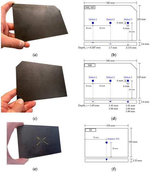
Figure 1.
Composite samples: (a) view of sample S45 from the front face; (b) specifications of samples S44 and S45; (c) view of the back face of specimen S48; (d) defect specifications of sample S48; (e) view of the front face of sample S5; and (f) specifications of sample S5.
A view of the back face of sample S48 is presented in Figure 1c (the back views of samples S44 and S45 are similar). Sample S48 contains 6 inserts, some of which are superposed as depicted in Figure 1d. For instance, defect 3 on sample S48 consists of 3 inserts located at different layers: the first one at a depth of z = 1.41 mm, the second one at z = 1.69 mm, and the third one at z = 1.98 mm.
The impacted samples have all approximately the same dimensions (measured thicknesses are slightly different) as seen in Table 1 and were impacted at the center following the drop-weight impact testing (16 mm diameter impactor) as described by the ASTM D7136 procedure [14]. A photograph of the front face of sample S5 can be seen in Figure 1e and its corresponding specification in Figure 1f. Impacted sample S9 is similar to S5, both have been impacted with an energy of 10 J, whilst samples S28 and S29 were impacted with energies of 12 and 15 J, respectively.
2.2. Data Acquisition
All samples were inspected in reflection mode, i.e., with the camera on the same side as the heating source, by pulsed thermography (PT) and line scan thermography (LST). In addition, they were also inspected in transmission mode, i.e., with the camera at the opposite side than the heating source as seen in Figure 2a, only by PT in order to estimate the thermal diffusivity of each plate.
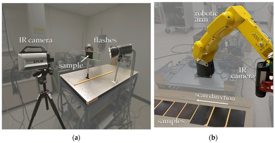
Figure 2.
Experimental setups: (a) pulsed thermography (in transmission mode); and (b) line scan thermography (in reflection mode).
2.2.1. Pulsed Thermography (PT)
Figure 2a presents a view of the experimental setup for the PT tests in transmission mode (used for the estimation of the thermal diffusivity of the samples as discussed in Section 2.3.4). For the reflection mode (not shown) the flashes are placed between the camera and the specimen. A high-definition cooled IR camera (FLIR X8501sc, NEdT < 20 mK, InSb, 3–5 μm, 1280 × 1024 pixels, linear Sterling cooling, lens focal length = 50 mm) and two xenon flashes (Balcar, 6.2 kJ per flash, pulse duration 2 ms @ FWHM) are used and synchronized through a PC. The camera is positioned 60 cm from the specimens and the flashes are placed at a distance of 25 cm from either the back or the front side of the specimens depending on the test mode (transmission or reflection, respectively) forming a 45° angle with respect to the sample surface. Samples were inspected one at a time (S44, S45, S48), in reflection and transmission modes. In all cases, thermographic sequences of 2000 frames at 42 fps were collected and processed as described in Section 2.3.1.
2.2.2. Line Scan Thermography (LST)
Figure 2b shows the experimental setup used for LST. The robot carries a thermographic head (Visiooimage inc. industrial line scan) holding an uncooled microbolometer camera (FLIR, 7.5–14 μm, NEdT < 30 mK, 640 × 480 pixels, lens focal length = 13.1 mm) and a heater. All three porosity samples together with the 4 impacted samples were inspected at once using different scanning speeds (5, 10, 25, 50, 125, and 250 mm/s). The scanning speed has an impact on the amount of energy that is delivered to the samples and hence on the maximum depth at which a defect can be detected. On one hand, if not enough energy is provided, e.g., at very high scanning speeds, the maximum depth that can be reached will be limited. On the other hand, longer heating, e.g., at very low scanning speeds, may worsen defect resolution due to excessive heating. It was determined that the optimal scanning speed is around 25 mm/s in this specific case, although it depends mainly on the depth of the defects. At scanning speeds much slower or faster than this, defects appear with lesser contrast. The camera was positioned at 267 mm from the sample and the heater at 10 mm from the sample surface with a power of 500 W.
2.3. Data Processing
2.3.1. Pulsed Thermography (PT)
In the case of PT, thermographic sequences are processed as depicted in Figure 3 using the MATLAB programming platform. Sample S45, as inspected by PT in reflection mode from the back face, is used as an example to illustrate the processing procedure. Figure 3a presents a thermogram at a given time arbitrarily chosen (0.35 s after the flash pulse in this case), in which a suspect area can be visually identified. From this thermogram, a region-of-interest (ROI) is manually selected around the identified anomaly (defect 1 in this case, see Figure 1b) and the whole sequence is cropped to contain only this ROI as shown in Figure 3b.
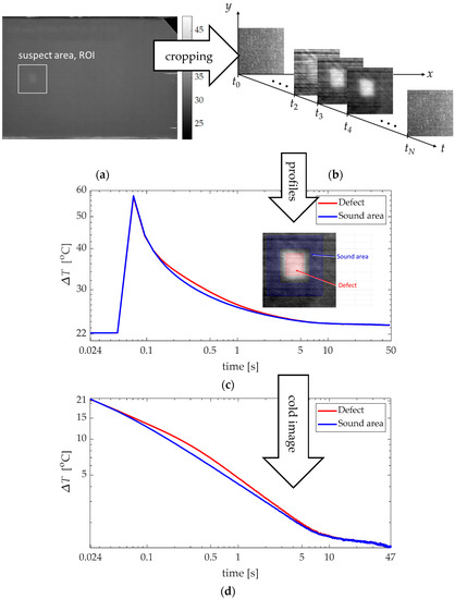
Figure 3.
Pulsed thermography processing (sample S45, defect 1): (a) thermogram at t = 0.35 s showing a suspect area (defect 1); (b) thermogram sequence corresponding to the ROI identified in (a); (c) sound area and defect temporal profiles for the complete sequence; and (d) profiles after cold image subtraction.
The next step is to manually select the defect area (red square inside the defect) and sound area (blue area around the defect) from one thermogram of the defect as shown in Figure 3c. Alternatively, semi-automatic identification of sound and defect areas (by locating the position of a point inside the defect) would also be possible as reported previously [15].
The temperature profiles are calculated as the average temperature value inside these areas (defect vs. sound) at each frame of the sequence. These profiles are shown in Figure 3c for the entire sequence, which includes images acquired before activating the flashes, i.e., cold images. The cold images are then averaged and subtracted from the whole sequence. This procedure allows the reduction of different types of noise, such as environmental reflections and fixed pattern noise. Cold image subtraction is also a requirement prior to the application of thermographic signal reconstruction. The cold images are then removed from the sequence resulting in the profiles shown in Figure 3d that will be subjected to further processing.
All identified ROIs (containing defects) are treated using the following advanced signal processing techniques [16]: thermographic signal reconstruction (TSR) [17,18], including first and second time derivatives; principal component thermography (PCT) [19]; and pulsed phase thermography [13,20].
In addition, two approaches were investigated to assess the impact of noise. First, PCT and PPT were applied to both: raw (unprocessed sequences) and TSR data in order to evaluate the denoising inherent to TSR. Second, the use of spatial filters was also examined through the use of Gaussian filters of two degrees with variances σ2 = 1 and 3.
2.3.2. Line Scan Thermography (LST)
In the case of LST, data are acquired in a dynamic configuration, i.e., the camera and the heating source (IR heater) move in tandem above the surface of the samples at a constant scanning speed. This allows reconstruction of a pseudo-static sequence following the procedure described in previous works [21,22]. It is also possible to process the dynamic sequences by PPT as described in [9,23].
The original thermographic data are in a three-dimensional (3D) sequence with frames represented in spatial coordinates x, y through time t. The complete sequence usually consists of several hundred frames. For the sake of clarity, Figure 4a shows only 4 representative thermograms arbitrarily selected at different times. It can be seen for instance that early in the sequence, i.e., at t1, the first plate (S44) can be completely seen, while the second plate (S48) is seen partially. As the scanning continues, plates appear and disappear from the camera field-of-view (FOV) as illustrated at different times (t2, t3, and t4). The acquisition ends after all plates are scanned and there is no longer any sample in the camera FOV.
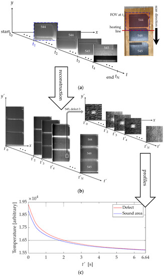
Figure 4.
LST processing: (a) dynamic sequence, line scan at 25 mm/s; (b) pseudo-static reconstructed sequence and ROI sequence showing defect 1 of sample S45; and (c) thermal profiles of defect 3 and the sound area around it.
The dynamic sequence is then recomposed in such a way that the original y dimension and time t are transposed as the observation time t′ and coordinate y′, respectively, whilst the x coordinate remains unchanged. The reconstructed pseudo-static matrix is shown in Figure 4b and consists of several images (equal to the spatial resolution in the scanning direction, the y coordinate in this example) distributed along the observation time t′. In the process, the positions of the reconstructed y′ lines are adjusted by interpolation to compensate for the lack of synchronization between the scanning speed and the camera frame rate.
The observation time, t′, which is the time during which every line of pixels along the y coordinate (in the direction of the scan) is registered by the camera after thermal stimulation, is calculated from the length Y (in mm) of the FOV in the direction of the scan and the scanning speed vy:
The length of the FOV in the scanning direction Y, is calculated by knowing the distance between the camera and the sample surface and the lens focal length.
For instance, for a lens with a focal length = 13.1 mm, with the camera located 267 mm from the sample and a scanning speed of vy = 25 mm/s: Y = 166.3 mm and t′ = 6.64 s.
An ROI surrounding defect 1 of specimen S45 can be identified in Figure 4b (white square in the thermogram at t′4) and then cropped from the reconstructed sequence showing the thermal evolution of the ROI through the observation time t′ as also seen in Figure 4b. The thermal profiles of defect vs. sound areas are shown in Figure 4c.
After reconstruction, the LST pseudo-static matrix can be processed using advanced signal processing techniques such as TSR, PCT, and PPT, as is conducted with PT [22]. Examples of signal processing of LST (and PT) data are presented in Section 3.
2.3.3. Contrast-to-Noise Ratio (CNR)
The contrast-to-noise ratio (CNR) is proposed as an objective means to provide a quantitative assessment of noise. Several CNR definitions may be found in the scientific literature [15]. Nevertheless, there are no standards specifically related to infrared thermography. There is, however, a standard for the evaluation of digital detector array systems for industrial radiology [24] from which a proper CNR definition can be adapted for the purpose of this study:
where μd is the average level of the signal in the defect region; μSa is the average level of the signal in the sound area (around the defect); and σSa is the standard deviation of the sound area.
The CNR was calculated frame by frame using Equation (2) in search of the maximum value, CNRmax, and thus the frame presenting the “best” contrast. This procedure is depicted in Figure 5.
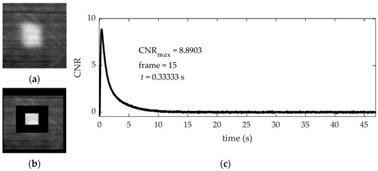
Figure 5.
Determination of the frame with maximum CNR (defect 1 from sample S45 by PT): (a) Raw thermogram arbitrarily selected; (b) same thermogram showing defect and sound areas; and (c) CNR profile over time.
Figure 5a displays a frame (arbitrarily selected) in which an anomaly can be identified, i.e., detect 1. The same frame showing the defect and sound (around the defect) areas, manually selected to estimate the CNR at every frame, is presented in Figure 5b. A transition zone is left between the defect and the sound area to reduce the effect of heat diffusion. Figure 5c shows the CNR variation frame by frame from which the CNRmax can be determined, together with its corresponding frame number and time.
2.3.4. Estimation of Thermal Diffusivity, α
The thermal diffusivity α, can be experimentally determined by exposing a sample of the material to a high-intensity short duration heat pulse in one face, while recording the temperature evolution from the opposite face, i.e., in transmission mode. This approach, originally proposed by Parker [25], is commonly referred to as the “Parker method” or the “Flash method”, and it counts with a standard test method E1461 [26] and standard practice E2585 [27] from the ASTM. According to these standards, the diffusivity can be obtained by solely knowing the specimen thickness L and estimating the time when the temperature reaches half the maximum value t1/2 [26]:
This technique was later refined using different time parameters (partial times) to consider heat losses. The resulting technique is called the partial times method [28], from which the following equations are proposed to estimate the diffusivity [29,30]:
Standard E1461 recommends employing small (from 6 to 30 mm in diameter) and thin (1 to 6 mm) circular discs to reduce non-uniform heating and to minimize heat losses and is strictly valid on measurements performed on fully dense (non-porous), homogeneous, and isotropic (opaque) materials. In the present study, the samples are anisotropic and non-homogeneous (i.e., CFRP), hence, results are of course subjected to incertitude. The samples however are relatively thin (3.4 mm) so heat losses are minimal, and although the samples are considerably larger (180 × 120 mm2) than what is suggested by the norm, the use of xenon flash lamps illuminating the whole surface aids in reducing non-uniform heating (when compared to laser spot stimulation). In any case, the results presented herein can be considered sufficiently accurate for the purpose of this work. More precise measurements of the diffusivity are out of the scope of this study.
2.3.5. Depth Estimation with the Phase
Defect characterization, i.e., the determination of the defect characteristics such as the depth, its thermo-physical properties, or its size, constitutes the ultimate purpose in IRT NDT since it provides a quantitative means to assess the impact of the presence of an anomaly. Nevertheless, it is not always necessary to implement defect characterization steps, many times the sole presence of a defect would be enough to determine if a given component needs to be repaired or replaced.
In the case of porosity and impact damage, it may be important to assess the severity and location of damage in the decision-making process. Pulsed phase thermography can be used to estimate the depth of defects by knowing the thermal diffusivity of the materials being inspected, and the defect’s blind frequency:
where C1 = 1.8 for the phase [13,31].
The blind frequency fb is defined as the maximum frequency at which a defect at a particular depth presents enough phase contrast to be detected. Phase contrast equals zero, Δϕ = 0, at frequencies higher than fb; whilst Δϕ will gradually increase for decreasing frequencies until reaching a maximum Δϕmax at fmax (which will depend on the depth of the defect) and then go down until reaching zero at f = 0 Hz.
3. Results and Discussion
3.1. Comparison of PT and LST through CNR Analysis
CNRmax values for all defects and processing techniques are shown in Table 2. The following figures summarize the results of different defects in the porosity samples selected in order to highlight the pros and cons of the different experimental methods (PT vs. LST), signal processing techniques (raw, TSR, PPT, and PCT), and filtering (unfiltered vs. Gaussian filtering).
Table 2.
Maximum CNR measured on porosity samples: comparison between unfiltered and filtered (Gaussian filter, σ2 = 1 and σ2 = 3).
Figure 6 aims to illustrate the difficulty in assessing the efficiency of defect detection under changing situations. Several images from this figure show apparently similar defect contrasts to the human eye, whether they are processed or not, or filtered or not. Profiles representing spatial variations through a horizontal line at the center of these images (dotted white line seen in the first image) are also included at the bottom of each image. Spatial profiles provide a hint of the noise level of images. For instance, TSR considerably denoises data following a synthetic data reconstruction after fitting. This is particularly evident with the phase calculated from TSR data, the 1st and the 2nd time derivatives (last three columns of the first line).
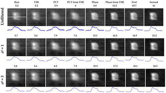
Figure 6.
Pulsed thermography. Impact of advanced signal processing and Gaussian filtering on single layer porosity at shallow depth: sample S44, front face, defect 1 (insert at z = 0.287 mm, thickness = 0.17 mm).
It can also be noted that filtering has some impact on image noise as seen by comparing unfiltered (first line in Figure 6) vs. filtered (second and third lines, for which the degree of Gaussian filtering changes from a variance σ2 = 1 to 3, respectively). Still, it is a difficult task to objectively assess denoising by visual examination of these images or even the respective spatial profiles.
The CNR is an interesting parameter that can be used as a criterium to quantitatively compare results. The images presented in Figure 6 correspond to the CNRmax values (estimated following the procedure presented in Section 2.3.3) for each technique. It can be observed that the CNR significantly increases with advanced signal processing (TSR, PCT, and PPT) and even further when fitted data, e.g., TSR, is used as input (instead of raw data) to PCT and PPT, as well as 1st and 2nd time derivatives.
Figure 7 presents LST results for the same defect presented in Figure 6 for PT, i.e., defect 1 in sample S45. At first glance, CNR values are considerably higher for PT. This was to be expected since a high-definition, high thermal resolution, cooled camera is used for PT, whilst a microbolometer uncooled camera is used for LST.
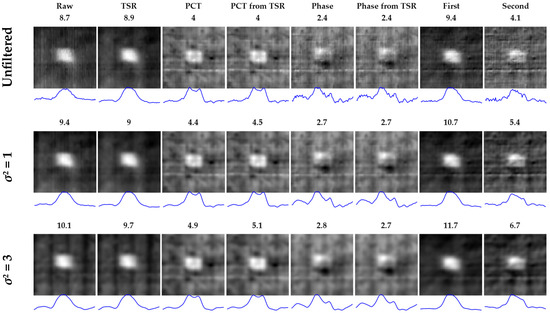
Figure 7.
Line scan thermography at 25 mm/s. Impact of advanced signal processing and Gaussian filtering on single layer porosity at shallow depth: sample S45, front face, defect 1 (insert at depth = 0.287 mm, thickness = 0.19 mm).
A second observation is that improvement in CNR is more erratic for LST. For instance, it actually worsens after processing in all cases with the exception of the 1st time derivative. This is probably related to the data reconstruction which may add some noise due to the dynamic scanning process. This needs to be further investigated.
Finally, as expected, Gaussian filtering improves CNR in all cases. The variance has a significant impact as observed from the two options studied herein (σ2 = 1 and 3). Nevertheless, two important observations should be pointed out. First, variance values were selected arbitrarily, using previous empirical knowledge from similar investigations. There must be an optimal variance that could be selected in order to improve defect contrast as much as possible. The determination of this optimal value would require further study, which is out of the scope of the present work. Second, any kind of spatial filtering modifies the input signal to some extent and may corrupt images if not selected properly. Hence, even though it is clear from the results presented herein that the CNR can be significantly improved using Gaussian filtering, additional research should be carried out to better assess the impact of filtering on defect contrast enhancement.
Figure 6 and Figure 7 illustrate the impact of advanced signal processing and filtering on noise reduction, i.e., on CNR values, for the case of a shallow defect, which could in fact be easily detected even without filtering or signal processing given that it is very close to the inspected surface (z = 0.285 mm). Deeper defects are more challenging as demonstrated next.
Figure 8 and Figure 9 include PT raw and processed results (the first 8 columns), as well as the best LST results, i.e., images with the highest CNRmax (the last two columns in Figure 8, and only the last column in Figure 9). Considering exclusively the impact of advanced signal processing applied to PT data (top line, excluding the last column) in Figure 8, it can be noticed that defect 1 of sample S48 would not be detected without processing as the raw result has a rather low defect contrast, i.e., CNRmax = 1.1. It is only after processing that the porosity area becomes clearly recognizable (roughly CNRmax ≥ 3.4). On the other hand, considering exclusively the impact of Gaussian filtering (first column in Figure 8), it can be concluded that filtering also improves the CNR although to a lesser extent than signal processing (at least for the kind of filter and variances utilized herein), passing from CNRmax = 1.1 without filtering, to CNRmax = 2.5 for a Gaussian filter with a variance σ2 = 1, and to CNRmax = 3.1 for a Gaussian filter with σ2 = 3. The striking combined effect of advanced signal processing and image filtering on defect contrast enhancement can be emphasized by comparing the raw result (the lowest CNR, top-left) to the second time derivative result (the highest CNR, bottom-right) improving the CNRmax from 1.1 to 11.8.
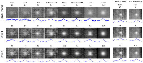
Figure 8.
Pulsed thermography vs. line scan thermography at 10 mm/s. Impact of advanced signal processing and Gaussian filtering on single layer porosity at intermediate depth: sample S48, front face, defect 1 (insert at depths = 1.69 mm, thickness = 0.16 mm).
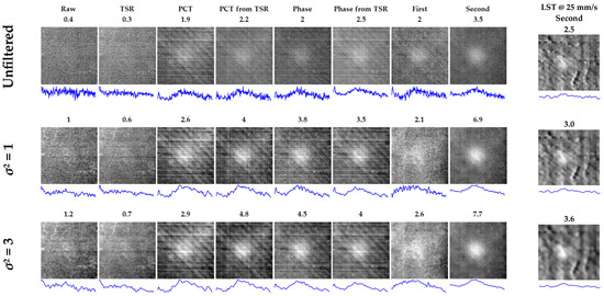
Figure 9.
Pulsed thermography vs. line scan thermography at 25 mm/s. Impact of advanced signal processing and Gaussian filtering on multilayer porosity at intermediate depth: sample S48, front face, defect 3 (inserts at depths = 1.41, 1.69, and 1.98 mm, thickness = 0.16 mm).
In the case of LST (last 2 columns in Figure 8), it is interesting to note that, contrary to PT, porosity can be detected by LST with good contrast without signal processing or filtering, CNRmax = 4.5 (see Table 2 for reference). This is due to a longer thermal stimulation in LST that allows heat diffusion to reach the defects and increase contrast. Signal processing does not improve CNR as drastically as PT (in some cases even worsens). The best results are obtained with TSR 1st time derivative (last column). A pattern of vertical lines can be perceived in the LST results. This pattern apparently corresponds to the grid in front of the heating IR lamp. Interestingly, the 1st time derivative removes this effect.
Figure 9 summarizes the results for defect 3 in sample S48. Even though both Figure 8 and Figure 9 present results for porosity at an intermediate depth, i.e., close to the middle thickness of sample S48, there are significant differences between them. Defect 1 (presented in Figure 8) is a single-layer porosity area located at z = 1.7 mm, whilst defect 3 (Figure 9) is composed of 3 superimposed porosity areas at different layers, z = 1.41, 1.69, and 1.98 mm (see Figure 1d for reference). As a result, CNRmax values of defect 1 (Figure 8) are higher than those of defect 3 (Figure 9).
Considering PT results for defect 3 (first 8 columns in Figure 9), as was the case for defect 1(Figure 8), signal processing and filtering have a major impact on improving defect contrast, as can be verified from the comparison of unfiltered raw (CNRmax = 0.4) vs. Gaussian filtered (σ = 3) second time derivative (CNRmax = 7.7) results. In the case of LST, contrary to defect 1 (Figure 8), defect 3 (Figure 9) cannot be clearly detected without signal processing as shown in the last column in Figure 9, which corresponds to the 2nd time derivative.
Figure 10 presents a notable example of the impact of signal processing and LST capabilities to detect deep features. As seen in Table 2, defect 3 in sample S45 is not detected by PT. On the other hand, it is possible to fairly (CNR around 3) detect this defect by LST but only after applying advanced signal processing. Figure 10 shows the results of PCT, which presented the highest CNRmax values.
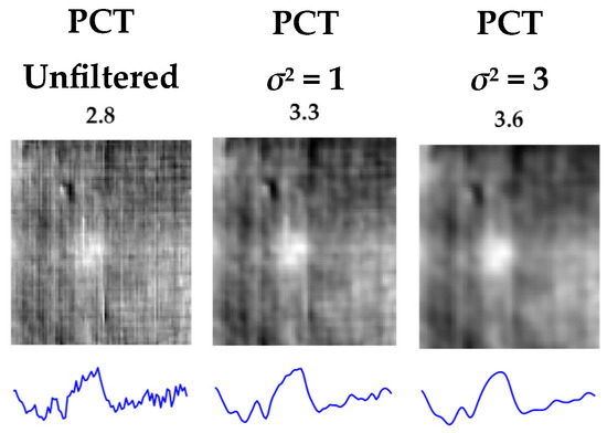
Figure 10.
Line scan thermography at 25 mm/s. Impact of advanced signal processing and Gaussian filtering on single layer porosity at the deepest depth: sample S45, defect 3 (insert at z = 3.115 mm, thickness = 0.19 mm).
It is not clear though why in this case the PCT (from raw data) shows the best CNR instead of other techniques, TSR 1st or 2nd time derivatives in particular.
Interestingly, as can be observed from Table 2, a slower scanning speed does not necessarily translates into an increase in defect contrast. For sample S48, CNR results for three scanning speeds (25, 10, and 5 mm/s) are listed. Although some improvement can be observed on defects 1 and 2 in sample S48 when slowing down from 25 to 10 mm/s, defect 3 is no longer detected at 10 mm/s. Further reducing the scanning speed (to 5 mm/s), worsen defect contrast in all cases, only defect 1 can be detected and with lesser contrast.
3.2. Thermal Diffusivity by the Flash Method
Figure 11 exhibits a representative example (sample S44) of the procedure used for the calculation of the thermal diffusivity using the flash method (PT in transmission mode) and partial times. The raw data (blue dots) are first fitted using the Savitzky–Golay filter (red dotted curve) seen in Figure 11a, from which the maximum temperature and the corresponding time tmax are obtained, followed by the calculation of the partial times: t1/3, t1/2, t2/3, and t5/6. The thermal diffusivity is then obtained from Equations (4) through (6), and finally averaged (αmean).
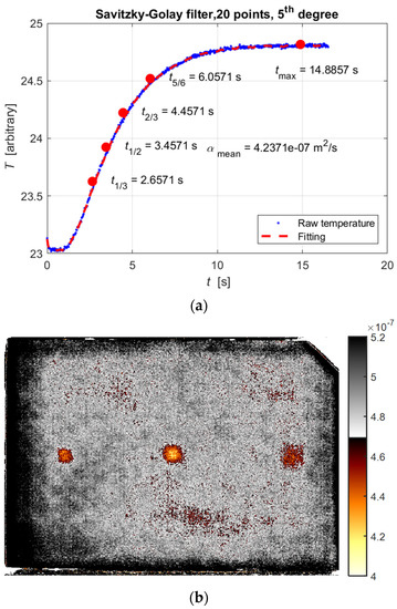
Figure 11.
Calculation of the thermal diffusivity by flash method and partial times (sample S44, front face): (a) raw data (points) and fitting (dotted line) result using the Savitzky–Golay filter; and (b) pixel-by-pixel diffusivity map.
The procedure is repeated for every pixel so a diffusivity map can be reconstructed as shown in Figure 11b, in which the three defects can be clearly identified as the thermal diffusivity is affected by the presence of the artificial porosity areas. From this figure, it can be observed that healthy areas have diffusivities above 4.7 × 10⁻⁷ m2/s (appearing mostly gray in Figure 11b), while defective areas are below this threshold (appearing mostly orange-yellow in Figure 11b).
The thermal diffusivity of all specimens was estimated following the same procedure. The average values for sound areas in all samples are summarized in the last column of Table 1.
3.3. Depth Estimation
As mentioned before (see Section 2.3.5), the sole requirement to retrieve the defect depth from PPT is the knowledge of the thermal diffusivity and the determination of the blind frequency. The thermal diffusivity for all specimens was estimated as described in the precedent section. The blind frequencies were obtained as follows.
Figure 12a presents an example of the estimation of the fb for defect 1 in sample S45. This graph shows the phase vs. frequency profiles obtained from raw data (blue and red dots corresponding to sound and defect areas, respectively), and the phase vs. frequency profiles obtained from TSR data (blue and red solid lines). The fb is determined as the first crossing point (starting at f = 0 Hz) between the defect and sound phase from TSR profiles, i.e., fb = 5.481 Hz. Replacing this and the measured thermal diffusivity value from Table 1 (i.e., α = 4.935 × 10⁻⁷ m2/s for sample S45) into Equation (5): zest = 0.3024 mm, which is relatively close to the actual z = 0.287 mm.
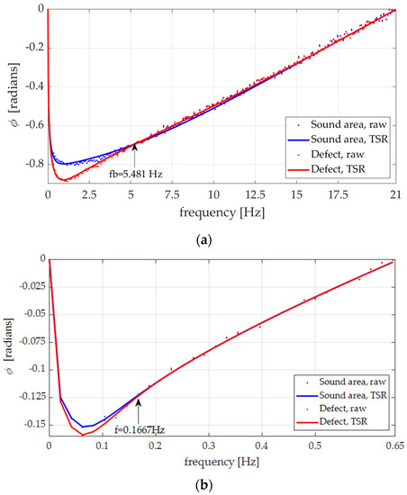
Figure 12.
Determination of the blind frequencies for depth estimation with the phase, plate S45 inspected: (a) defect 1 (depth = 0.287 mm); and (b) defect 2 (depth = 1.7 mm).
The depth of defect 2 in sample S45 was estimated in a similar way. Figure 12b shows the phase vs. frequency profiles. The blind frequency, in this case, is fb = 0.1667 Hz, and the estimated depth is zest = 1.734 mm, also close to the actual z = 1.7 mm. The depth of defect 3 could not be estimated since it was not detected as seen in Table 2.
The same procedure was followed to estimate the depth at different locations inside the damaged area of the impacted samples. Figure 13 shows the results for the impacted specimen S5. The phase profiles can be seen in Figure 13a, from which, the blind frequencies are extracted for each ROI. ROI1 is located at the left near the center of the plate as seen in Figure 13b, which presents a phasegram at a very low frequency (f = 0.02 Hz) showing the deepest features (i.e., ROI1). As the frequency increases, the phasegrams show more and more shallow features as seen in Figure 13c–e.
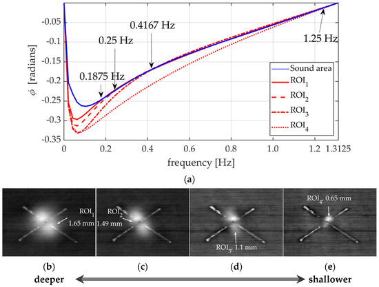
Figure 13.
Specimen S5. Determination of the depth at different regions of impacted specimen S5: (a) phase profiles of the sound area (blue) and the ROIs (red) showing the blind frequencies corresponding to the ROIs depths; phasegrams at f = (b) 0.02; (c) 0.08; (d) 0.1875; and (e) 0.5 Hz, showing selected ROIs and their estimated depths.
The blind frequency of ROI1 can be obtained from the phase profiles in Figure 13a, i.e., fb = 0.1875 Hz. The depth can then be estimated from Equation (7) using this value and the thermal diffusivity reported in Table 1, which gives zest = 1.65 mm. Similarly, depths for the other ROIs were estimated as 1.49, 1.1, and 0.65 mm for ROI2, ROI3, and ROI4, respectively, as shown in Figure 13c–e.
Finally, impact damage on all four samples can be seen in Figure 14. In Figure 14a, the damaged area is zoomed-in and rotated 90° with respect to the white rectangle shown in Figure 14b to be compared to Figure 13b. Both images show roughly the same area. The PT result in Figure 13b shows evidently more details (e.g., composite fibers) given the higher spatial resolution and sensitivity of the cooled camera, but the damage appears with higher contrast in the LST result presented in Figure 14b. This is because the sample was heated much longer by LST than for PT.
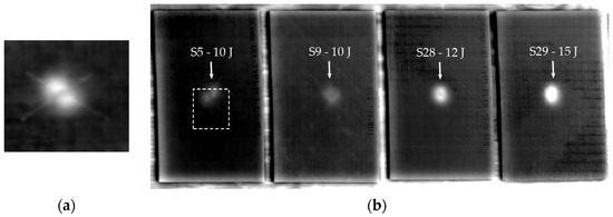
Figure 14.
Impacted samples: LST at 10 mm/s: (a) close-up of impact damage on sample S5 rotated 90° counterclockwise with respect to the rectangular area in the image at the right; and (b) reconstructed thermogram showing all four impacted samples approximately 0.5 s after heating.
Figure 14b shows a visual (subjective) comparison of the degree of damage for increasing impact energies. For instance, 10 J impacts (samples S5 and S9) show similar gray levels. Nevertheless, gray levels at the damaged areas increase with the impact energy as clearly seen when comparing energies of 10, 12, and 15 J.
4. Conclusions
The main purpose of this paper was twofold. First, to quantitatively evaluate the performance of LST for the detection of porosity and BVID in carbon fiber composites. Robotic LST systems have the advantage of being more adapted for online inspection during the production of flat and complex-shaped aerospace components. This is currently of great interest in the aerospace industry in order to reduce inspection times without compromising defect detection effectiveness. Second, to probe that porosity and impact damage can be quantified using IRT methods. For this second goal, a PT approach was selected since a defect characterization procedure exists using advanced signal processing, i.e., pulsed phase thermography (PPT). In addition, the thermal diffusivity of the material was measured as a first step toward the determination of depth by PPT.
The performance of LST with an uncooled microbolometer camera was evaluated with respect to PT with a high-definition camera, which can be considered the gold standard in IRT. A set of academic plates containing artificial porosity and BVID was inspected using both approaches. The CNR was used as a quantitative parameter to objectively evaluate defect contrast. It was calculated frame by frame for all defects and all processing techniques, so the maximum values CNRmax were found for each approach. Table 2 summarizes the measured CNRmax. Globally, CNR values were greater for PT than for LST, as expected given the differences in camera spatial resolution and sensitivity between setups, and also because a static configuration allows recording of thermal cooling longer than a dynamic configuration, which further improves defect contrast. Nevertheless, there were some situations where LST performed better than PT. Notably, defect 3 in sample S45, which is a single-layer artificial porosity area at z = 3.115 mm (Figure 10), was only detected by LST (at 25 mm/s) and not by PT. This is because with LST the sample was heated longer than with the flashes. Hence, the energy delivered to the sample was sufficient to reach this defect and produce enough defect contrast. The use of a longer pulse, using halogen lamps, for example, would most probably improve results for deeper defects when using a static configuration.
The application of advanced signal processing significantly improved CNR in all cases but more significantly in PT. Spatial filters also improved CNR values but to a lesser extent. The combined effect of advanced processing and Gaussian filtering can be clearly appreciated for instance in Figure 9, which presents the case of multilayer porosity at the middle thickness of the sample that shows an improvement of CNRmax from 0.4 (not detected) to 7.7 (clearly detected) after processing and filtering. Further research should be carried out to investigate the limiting variance values of Gaussian filtering considering that any spatial filter modifies images to some extent.
This research study has clearly demonstrated that LST (with a microbolometer camera) can be used for the detection of porosity and BVID in composite materials with performance comparable to PT (with a high-definition cooled camera), which could potentially improve inspection times in the aerospace manufacturing industry. It is also demonstrated that porosity and impact damage in composites can be quantified from PPT, provided that the thermal diffusivity is known or can be measured, e.g., by PT in transmission mode. Future works should explore the possibility of quantifying defects from LST, further optimize inspection time and assess the impact of geometry on non-planar components.
Author Contributions
Conceptualization, P.S., M.K., X.P.V.M., T.B., A.K., S.H. and C.I.-C.; methodology, P.S., M.K., X.P.V.M., S.H. and C.I.-C.; software, M.K. and C.I.-C.; validation, P.S., M.K., X.P.V.M., T.B., A.K., S.H. and C.I.-C.; formal analysis, P.S., M.K., X.P.V.M. and C.I.-C.; investigation, P.S., M.K., X.P.V.M. and C.I.-C.; resources, P.S., M.K. and X.P.V.M.; data curation, C.I.-C.; writing—original draft preparation, C.I.-C.; writing—review and editing, T.B., P.S., M.K. and S.H.; supervision, T.B. and X.P.V.M.; project administration, T.B. and M.K.; funding acquisition, T.B., M.K. and X.P.V.M. All authors have read and agreed to the published version of the manuscript.
Funding
This research was funded by WALLONIA REGION, grant number C8188, R&D project, Laboratoire Digital for Composite LDCOMP, 2020–2023.
Institutional Review Board Statement
Not applicable.
Informed Consent Statement
Not applicable.
Data Availability Statement
Not applicable.
Acknowledgments
The authors wish to thank Wallonia Region for its support in R&D.
Conflicts of Interest
The authors declare no conflict of interest.
References
- Park, S.-J.; Seo, M.-K. Chapter 8-Composite Characterization. Interface Sci. Technol. 2011, 18, 631–738. [Google Scholar] [CrossRef]
- Madenci, E.; Onuralp Ozkili, Y. Free vibration analysis of open-cell FG porous beams: Analytical, numerical and ANN approaches. Steel Compos. Struct. 2021, 40, 157–173. [Google Scholar] [CrossRef]
- Katunin, A.; Wronkowicz-Katunin, A.; Danek, W.; Wyleżoł, M. Modeling of a realistic barely visible impact damage in composite structures based on NDT techniques and numerical simulations. Compos. Struct. 2021, 267, 113889. [Google Scholar] [CrossRef]
- Daniel, I.M.; Wooh, S.C.; Komsky, I. Quantitative porosity characterization of composite materials by means of ultrasonic attenuation measurements. J. Nondestruct. Eval. 1992, 11, 1–8. [Google Scholar] [CrossRef]
- Gusenbauer, C.; Reiter, M.; Plank, B.; Salaberger, D.; Senck, S.; Kastner, J. Porosity Determination of Carbon and Glass Fibre Reinforced Polymers Using Phase-Contrast Imaging. J. Nondestruct. Eval. 2018, 38, 1–10. [Google Scholar] [CrossRef]
- Francesconi, L.; Taylor, M.; Bertoldi, K.; Baldi, A. Static and Modal Analysis of Low Porosity Thin Metallic Auxetic Structures Using Speckle Interferometry and Digital Image Correlation. Exp. Mech. 2017, 58, 283–300. [Google Scholar] [CrossRef]
- Scislo, L. Single-Point and Surface Quality Assessment Algorithm in Continuous Production with the Use of 3D Laser Doppler Scanning Vibrometry System. Sensors 2023, 23, 1263. [Google Scholar] [CrossRef]
- Hendorfer, G.; Mayr, G.; Zauner, G.; Haslhofer, M.; Pree, R. Quantitative determination of porosity by active thermography. AIP Conf. Proc. 2007, 894, 702–708. [Google Scholar] [CrossRef]
- Moran, J.; Rajic, N. Remote line scan thermography for the rapid inspection of composite impact damage. Compos. Struct. 2018, 208, 442–453. [Google Scholar] [CrossRef]
- Ibarra-Castanedo, C.; Maldague, X.P.V. Infrared Thermography. In Handbook of Technical Diagnostics; Czichos, H., Ed.; Springer: Berlin/Heidelberg, Germany, 2013. [Google Scholar] [CrossRef]
- Maldague, X.P. Nondestructive Testing Handbook. 3. Infrared and Thermal Testing; American Society for Nondestructive Testing: Columbus, OH, USA, 2001. [Google Scholar]
- Ley, O.; Godinez-Azcuaga, V. Line scanning thermography and its application inspecting aerospace composites. In Proceedings of the 5th International Symposium on NDT in Aerospace, Singapore, 13–15 November 2013; pp. 13–15. Available online: http://www.ndt.net/article/aero2013/content/papers/48_Godinez-Azcuaga.pdf (accessed on 9 May 2023).
- Ibarra-Castanedo, C.; Maldague, X. Pulsed phase thermography reviewed. Quant. InfraRed Thermogr. J. 2004, 1, 47–70. [Google Scholar] [CrossRef]
- ASTM D7136/D7136M−15; Standard Test Method for Measuring the Damage Resistance of a Fiber-Reinforced Polymer Matrix Composite to a Drop-Weight Impact Event. ASTM International: West Conshohocken, PA, USA, 2022. [CrossRef]
- Usamentiaga, R.; Ibarra-Castanedo, C.; Maldague, X. More than Fifty Shades of Grey: Quantitative Characterization of Defects and Interpretation Using SNR and CNR. J. Nondestruct. Eval. 2018, 37, 25. [Google Scholar] [CrossRef]
- Ibarra-Castanedo, C.; Piau, J.M.; Guilbert, S.; Avdelidis, N.P.; Genest, M.; Bendada, A.; Maldague, X.P. Comparative study of active thermography techniques for the nondestructive evaluation of honeycomb structures. Res. Nondestruct. Eval. 2009, 20, 1–31. [Google Scholar] [CrossRef]
- Shepard, S.M.; Lhota, J.R.; Rubadeux, B.A.; Wang, D.; Ahmed, T. Reconstruction and enhancement of active thermographic image sequences. Opt. Eng. 2003, 42, 1337–1342. [Google Scholar] [CrossRef]
- Balageas, D.L. Defense and illustration of time-resolved pulsed thermography for NDE. Quant. InfraRed Thermogr. J. 2012, 9, 3–32. [Google Scholar] [CrossRef]
- Rajic, N. Principal component thermography for flaw contrast enhancement and flaw depth characterisation in composite structures. Compos. Struct. 2002, 58, 521–528. [Google Scholar] [CrossRef]
- Maldague, X.P.; Marinetti, S. Pulse Phase Infrared Thermography. J. Appl. Phys. 1996, 79, 2694–2698. [Google Scholar] [CrossRef]
- Ibarra-Castanedo, C.; Servais, P.; Ziadi, A.; Klein, M.; Maldague, X. RITA-Robotized Inspection by Thermography and Advanced processing for the inspection of aeronautical components. In Proceedings of the 12th International Conference on Quantitative Infrared Thermography, Bordeaux, France, 7–11 July 2014; Available online: https://www.ndt.net/?id=17748 (accessed on 9 May 2023).
- Khodayar, F.; Lopez, F.; Ibarra-Castanedo, C.; Maldague, X. Optimization of the inspection of large composite materials using robotized line scan thermography. J. Nondestruct. Eval. 2017, 36, 32. [Google Scholar] [CrossRef]
- Gray, J.; Woodrow, M.; Rosalie, C.; Rajic, N. Comparative Evaluation of a High Operating Temperature Midwave Infrared Detector for Automated Non-Destructive Inspection of Composite Damage. Mater. Res. Proc. 2021, 18, 29–36. [Google Scholar] [CrossRef]
- ASTM E2737−10; Standard Practice for Digital Detector Array Performance Evaluation and Long-Term Stability. ASTM International: West Conshohocken, PA, USA, 2018. [CrossRef]
- Parker, W.J.; Jenkins, R.J.; Butler, C.P.; Abbott, G.L. Flash Method of Determining Thermal Diffusivity, Heat Capacity, and Thermal Conductivity. J. Appl. Phys. 1961, 32, 1679. [Google Scholar] [CrossRef]
- ASTM E1461−13; Standard Test Method for Thermal Diffusivity by the Flash Method. ASTM International: West Conshohocken, PA, USA, 2022. [CrossRef]
- ASTM E2585−09; Standard Practice for Thermal Diffusivity by the Flash Method. ASTM International: West Conshohocken, PA, USA, 2022. [CrossRef]
- Degiovanni, A. Diffusivité et méthode flash. Rev. Générale Therm. 1977, 185, 420–442. [Google Scholar]
- Balageas, D.L. Nouvelle méthode d’interprétation des thermogrammes pour la détermination de la diffusivité thermique par la méthode impulsionnelle (méthode “flash”). Rev. Phys. Appl. 1982, 17, 227–237. [Google Scholar] [CrossRef]
- Hay, B.; Filtz, J.-R.; Batsale, J.-C. Mesure de la diffusivité thermique par la méthode flash. Tech. Ing. 2004, R2955, V1. [Google Scholar] [CrossRef]
- Thomas, R.L.; Pouch, J.J.; Wong, Y.H.; Favro, L.D.; Kuo, P.K. Subsurface Flaw Detection in Metals by Photoacustic Microscopy. J. Appl. Phys. 1980, 51, 1152–1156. [Google Scholar] [CrossRef]


Disclaimer/Publisher’s Note: The statements, opinions and data contained in all publications are solely those of the individual author(s) and contributor(s) and not of MDPI and/or the editor(s). MDPI and/or the editor(s) disclaim responsibility for any injury to people or property resulting from any ideas, methods, instructions or products referred to in the content. |
© 2023 by the authors. Licensee MDPI, Basel, Switzerland. This article is an open access article distributed under the terms and conditions of the Creative Commons Attribution (CC BY) license (https://creativecommons.org/licenses/by/4.0/).