Computational Dynamics of Multi-Rigid-Body System in Screw Coordinate

Abstract

This paper investigates the kinematics and dynamics of multi-rigid-body systems in screw form. The Newton–Euler dynamics equations are established in screw coordinates. All forces and torques of the multi-rigid-body system can be solved straightforwardly since they are explicit in the form of screw coordinates. The displacement and acceleration are unified in matrix form, which associates the kinematics and dynamics with variable of velocity. A one-step numerical algorithm only is needed to solve the displacements and accelerations. As a result, all absolute displacements, velocities, and accelerations are directly obtained by one kinematic equation. The kinematics and dynamics of Gough–Stewart platform validate this the method. In this paper, the kinematics and dynamics are carried out with the example of a Gough–Stewart platform, which represents the most complex multi-rigid-body system, to verify the computational dynamics method. The proposed algorithm is also fit for the kinematics and dynamics modeling of other multi-rigid-body systems.

1. Introduction

It is well known that a multi-rigid-body system is normally a complex system with many links and joints and is fundamental for mechanism research in robotics, spacecraft, and bionic areas. Studies of multi-rigid-body systems can neglect the flexibility of the bodies and focus on the kinematic and dynamic performance of the mechanisms. Extensive research has proposed a series of theoretical models of multi-rigid-body systems. Parallel mechanisms are common multi-rigid-body systems with high loading ability, good dynamic response, and precise motion. The Gough–Stewart platform as a common parallel mechanism is proposed as a flight simulator by Gough and Stewart [1,2,3], which has high flexibility. Therefore, the study of the kinematics and dynamics of the Gough–Stewart platform is vital research topics for its application.

Dynamics analysis has theoretical and practical significance for realizing robot control, stability in motion, and optimization in structure. Scholars presented some dynamics methods for parallel mechanisms. The widely-used methods for multi-rigid-body system dynamics mainly include Lagrange equation [4,5], Newton–Euler equation [6], virtual work principle equation [7,8], Kane equation [9], and Gibbs–Appell equation [10]. The Newton-Euler dynamics equation for the Gough–Stewart platform, which is based on the vector method and proposed by Dasgupta, is a classic algorithm in dynamics modeling [11,12]. Newton-Euler equations can express the rotational and translational motion of a rigid body in the absolute coordinate system. Through a single equation with six components in the form of column vectors and matrix, the forces and moments acting on the rigid body and the motion of the center of mass of a rigid body can be combined [13,14,15]. Gallardo-Alvarado [16,17] proposed dynamics analysis of parallel mechanisms by screw coordinates and the principle of virtual work. The analysis of a multi-rigid-body system is usually solved through analytical methods in classical mechanics and vector equations [18,19,20,21].

The displacement, velocity, and acceleration obtained in kinematics are essential information for dynamics modeling. To describe the kinematics of a mechanism, the translational and rotational motions should be expressed with a suitable mathematical framework in a relatively general way [22,23]. Meanwhile, there are also several finite solutions corresponding to different configurations of a multi-rigid-body system [24,25,26]. The kinematics modeling of a multi-rigid-body system can be simplified by resorting to screw coordinates. Many researchers have utilized screw coordinates in kinematics analysis [27,28] of parallel mechanisms.

This paper focuses on the kinematics and dynamics of a multi-rigid-body system by the Newton–Euler method in screw coordinate. From kinematics analysis, the absolute displacement, velocity, and acceleration of each joint and link can be derived in the absolute coordinate frame, which can be applied directly in dynamics. This method would be much clearer and more straightforward not only for the inverse dynamics problem but also for the derivation of closed-form dynamics formulae.

2. Kinematics of a Multi-Rigid-Body System

This section presents the method for establishing the kinematics of a multi-rigid-body system based on screw coordinates. Velocity screw is defined to unify the angular velocity and linear velocity of a joint. With the velocity screw equation, the relative velocity of each joint can be obtained. Then, both displacement and acceleration are calculated by a one-step numerical method. Based on the linear superposition principle, the absolute displacement, velocity, and acceleration of each joint can be derived uniformly in screw coordinates.

2.1. Relative Displacement, Velocity and Acceleration of Each Joint

In Figure 1a, for a multi-rigid-body system, there are $p$ kinematic chains each of which has $n$ joints. In the multi-rigid-body system, $L$ represents a link, $j$ represents a joint and $loop$ represents a kinematic chain. As shown in Figure 1b, suppose $L_{i-1}$ and $L_{i-2}$ are two rigid bodies in a serial kinematic chain which are connected by joint $j_{i-1}$.

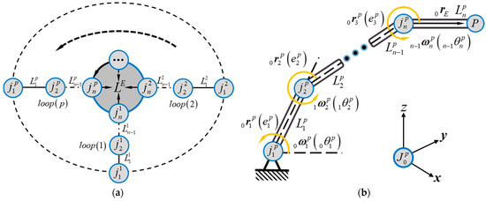
Figure 1. A multi-rigid-body system: (a) multi-rigid-body system; (b) a serial kinematic chain.

The dual 3-dimensional vectors, ${}_0\mathit{\omega }_1^p$ and ${}_0\mathit{v}_1^p$, can fully determine the motion of link $L_1^p$. Its velocity screw vector can be defined as

$${}_0\mathit{V}_1^p=\left[\begin{array}{c}{}_0\mathit{\omega }_1^p\\ {}_0\mathit{v}_1^p\end{array}\right]$$

(1)

where ${}_0\mathit{\omega }_1^p$ is the relative angular velocity vector of joint $j_1^p$ with respect to the grounded link 0, ${}_0\mathit{v}_1^p$ is the relative linear velocity of a point on the link $L_1^p$ with its extended body that is passing through the origin of the absolute coordinate frame at this instant.

The 3-dimensional vector ${}_0\mathit{v}_1^p$ can be expressed by ${}_0\mathit{v}_1^p={}_0\mathit{r}_1^p\times {}_0\mathit{\omega }_1^p$ where ${}_0\mathit{r}_1^p$ is the position vector of joint $j_1^p$ with respect to the origin of the grounded coordinate frame.

Suppose $\Vert {\mathit{e}}_1^p\Vert =1$, Equation (1) can be rewritten as

$${}_0\mathit{V}_1^p={}_0\mathit{\omega }_1^p\left[\begin{array}{c}{\mathit{e}}_1^p\\ {}_0\mathit{r}_1^p\times {\mathit{e}}_1^p\end{array}\right]$$

(2)

where ${\mathit{e}}_1^p$ is the direction vector of joint $j_1^p$ in the absolute coordinate frame, and ${}_0\mathit{\omega }_1^p$ is the relative angular speed of joint $j_1^p$ in the absolute coordinate frame. Let

$${\mathsf{\$}}_1^p=\left[\begin{array}{c}{\mathit{e}}_1^p\\ {}_0\mathit{r}_1^p\times {\mathit{e}}_1^p\end{array}\right]$$

(3)

where ${\mathsf{\$}}_1^p$ is the unit screw of joint $j_1^p$.

Substituting Equation (3) into Equation (2) yields

$${}_0\mathit{V}_1^p={}_0\mathit{\omega }_1^p{\mathsf{\$}}_1^p$$

(4)

For a kinematic chain $loop(p)$ shown in Figure 1a, based on the linear combination, the kinematics of the end joint $j_1^p$ can be expressed as:

$$\{\begin{array}{l}{}_0\mathit{\omega }_n^p={}_0\mathit{\omega }_1^p+{}_1\mathit{\omega }_2^p+{}_2\mathit{\omega }_3^p+\cdots +{}_{n-2}\mathit{\omega }_{n-1}^p+{}_{n-1}\mathit{\omega }_n^p\\ {}_0\mathit{v}_n^p={}_0\mathit{v}_1^p+{}_1\mathit{v}_2^p+{}_2\mathit{v}_3^p+\cdots +{}_{n-2}\mathit{v}_{n-1}^p+{}_{n-1}\mathit{v}_n^p\end{array}$$

(5)

In accordance with Equation (2), the forward kinematics of a single kinematic chain can be rewritten as:

$${}_0\mathit{V}_n^p={\displaystyle \sum _{i=0}^n{}_i\mathit{V}_{i+1}^p}={\mathit{S}}^p{\mathit{\omega }}^p$$

(6)

where

$${\mathit{S}}^p=\left[\begin{array}{cccc}{\mathsf{\$}}_1^p& {\mathsf{\$}}_2^p& \cdots & {\mathsf{\$}}_n^p\end{array}\right]$$

(7)

which represents the unit screw matrix of the single kinematic chain $loop\left(p\right)$

And

$${\mathit{\omega }}^p={\left[\begin{array}{cccc}{}_0\mathit{\omega }_1^p& {}_1\omega _2^p& \cdots & {}_{n-1}\omega _n^p\end{array}\right]}^T$$

(8)

where ${}_{n-1}\omega _n^p$ is the relative angular speed of the link $L_n^p$ with respect to the link $L_{n-1}^p$ connecting joint $j_{n-1}^p$.

With the definition of the twist matrix and Equation (6), the velocity screw equation of a multi-rigid-body system would be obtained,

$$\mathit{S}\mathit{\omega }=\mathit{V}$$

(9)

where

$$\mathit{S}=\mathrm{diag}{\left[\begin{array}{cccc}{\mathit{S}}^1& {\mathit{S}}^2& \cdots & {\mathit{S}}^p\end{array}\right]}_{6p\times 6p}$$

(10)

in which ${\mathit{S}}^p$ is the unit screw matrix of the single kinematic chain $loop\left(p\right)$, and $\mathrm{diag}[ ]$ is a diagonal matrix of ${\mathit{S}}^1,{\mathit{S}}^2,\cdots ,{\mathit{S}}^p$.

and

$$\mathit{\omega }={\left[\begin{array}{cccc}{\left({\mathit{\omega }}^1\right)}^T& {\left({\mathit{\omega }}^2\right)}^T& \cdots & {\left({\mathit{\omega }}^p\right)}^T\end{array}\right]}_{6p\times 1}^T$$

(11)

in which ${\mathit{\omega }}^p$ is the vector of relative angular speeds of all joints in the single kinematic chain $loop\left(p\right)$, and

$$\mathit{V}={\left[\begin{array}{cccc}{\left({}_0\mathit{V}_n^1\right)}^T& {\left({}_0\mathit{V}_n^2\right)}^T& \cdots & {\left({}_0\mathit{V}_n^p\right)}^T\end{array}\right]}_{6p\times 1}^T$$

(12)

in which ${}_0\mathit{V}_n^p$ is the vector of the absolute velocity screw of the nth joint in the single kinematic chain $loop\left(p\right)$. Equation (10) is the screw matrix of the multi-rigid-body system. Equation (11) is a velocity vector composed of the relative angular speeds of each generalized joint with respect to its previous link. Equation (12) is the velocity vector of each end joint in the absolute coordinate frame.

With Equation (6), when the kinematics of the terminal link $j_n$ is specified, its inverse kinematics of the multi-rigid-body system can be derived,

$${\mathit{S}}^T\mathit{S}\mathit{\omega }={\mathit{S}}^T\mathit{V}$$

(13)

When $\left|{\mathit{S}}^T\mathit{S}\right|=0$, the multi-rigid-body system is either redundantly actuated or in singularity configuration. Otherwise, we gain the angular speeds of all joints from Equation (13):

$$\mathit{\omega }={\left[{\mathit{S}}^T\mathit{S}\right]}^{-1}{\mathit{S}}^T\mathit{V}$$

(14)

where ${\left[{\mathit{S}}^T\mathit{S}\right]}^{-1}{\mathit{S}}^T$ is called the pseudo inverse of screw matrix $\mathit{S}$. Equation (14) represents the inverse velocity of the multi-rigid-body system. Based on Equation (14), we get the steps to calculate the inverse kinematics of a multi-rigid-body system below:

• With the initial condition consisting of position angles ${}_{n-1}\mathit{\theta }_n^p\left(t=0\right)$ and structure parameters $R$, $r$, and $l_n^p$, the unit screw matrix $\mathit{S}\left(0\right)$ of the multi-rigid-body system at time $t=0$ can be gained first.
• Substituting $\mathit{S}\left(0\right)$ into Equation (14) and with the twist matrix ${\mathsf{\$}}_n^p$ of the end joint $j_n^p$ in Equation (7) being known, the relative angular velocity of each joint $\mathit{\omega }\left(0\right)$ at time $t=0$ can be derived.
• With the initial conditions consisting of position and velocity, the parameters of ${\mathsf{\$}}_n^p\left(k\right)$ from Equation (10) and $\mathit{\omega }\left(k\right)$ from Equation (14) could be updated by steps 1 and 2 where $t=0$ is replaced by $t=k\Delta t$:

  $${}_{n-1}\mathit{\theta }_n^p\left(\left(k+1\right)\Delta t\right)={}_{n-1}\mathit{\theta }_n^p\left(k\Delta t\right)+\Delta t\mathit{\omega }\left(k\right)$$

  (15)

  where $k=1,2,\cdots$.

With the unit screw matrix $\mathit{S}\left(k\right)$, the position vector, ${}_0\mathit{r}_n^p$, and orientation vector, ${\mathit{e}}_n^p$, of each joint can be deduced from Equation (14).

2.2. Absolute Displacement, Velocity, and Acceleration of Each Joint

Due to the linear superposition principle, the absolute velocity of the nth joint at the absolute coordinate frame is expressed by

$${}_0\mathit{V}_n\left(k+1\right)={\displaystyle \sum _{i=1}^n{}_{i-1}\mathit{V}_i\left(k+1\right)}$$

(16)

Suppose ${}_0\mathit{D}_n=\left[\begin{array}{c}{}_0\mathit{\theta }_n^p\\ {}_0\mathit{d}_n^p\end{array}\right]$, in which ${}_0\mathit{D}_n$ is the absolute displacement vector of each joint that consists of absolute angular displacement ${}_0\mathit{\theta }_n$ and absolute linear displacement ${}_0\mathit{d}_n$. Suppose ${}_0\mathit{A}_n=\left[\begin{array}{c}{}_0\mathit{\beta }_n\\ {}_0\mathit{a}_n\end{array}\right]$, in which ${}_0\mathit{A}_n$ is the absolute acceleration vector of each joint that consists of absolute angular acceleration ${}_0\mathit{\beta }_n$ and absolute linear acceleration ${}_0\mathit{a}_n$. The absolute displacement and acceleration of each joint at the absolute coordinate frame can be expressed by the simplest one-step numerical algorithm,

$$\{\begin{array}{l}{}_0\mathit{D}_n\left(k+1\right)={}_0\mathit{D}_n\left(k\right)+\Delta t{}_0\mathit{V}_n\left(k\right)\\ {}_0\mathit{A}_n\left(k+1\right)=\frac{{}_0\mathit{V}_n\left(k+1\right)-{}_0\mathit{V}_n\left(k\right)}{\Delta t}\end{array}$$

(17)

The absolute velocity screw matrix ${}_0\mathit{V}_n$, the absolute displacement vector ${}_0\mathit{D}_n$, and the absolute acceleration vector ${}_0\mathit{A}_n$ can be obtained by calculating the angular displacement ${}_{n-1}\mathit{\theta }_n^p\left(t=0\right)$ with Equation (15). The results can be applied to the kinematics analysis of any point on a single-rigid-body.

2.3. Absolute Displacement, Velocity and Acceleration of Each Rigid-Body

Suppose there is a point $P$ on the rigid-body $L_n^p$, and the velocity of the point $P$ on the rigid-body $L_n^p$ is hence represented as

$${}_0\mathit{v}_n^P={}_0\mathit{v}_n+{}_0\mathit{\omega }_n\times {}_0\mathit{r}_P$$

(18)

where ${}_0\mathit{r}_P$ indicates the position vector of the point $P$ in the absolute ground coordinate frame 0.

For a kinematic chain $loop(p)$ shown in Figure 1b, the absolute angular and linear velocities of the point $P$ on the rigid-body $L_n^p$ can be expressed as:

$$\{\begin{array}{l}{}_0\mathit{\omega }_n^P={}_0\mathit{\omega }_1^p+{}_1\mathit{\omega }_2^p+{}_2\mathit{\omega }_3^p+\cdots +{}_{n-2}\mathit{\omega }_{n-1}^p+{}_{n-1}\mathit{\omega }_n^p\\ {}_0\mathit{v}_n^P={}_0\mathit{v}_1^p+{}_1\mathit{v}_2^p+{}_2\mathit{v}_3^p+\cdots +{}_{n-2}\mathit{v}_{n-1}^p+{}_{n-1}\mathit{v}_n^p+{}_0\mathit{\omega }_n^P\times {}_0\mathit{r}_P\end{array}$$

(19)

Consequently, the velocity of a point $P$ on the rigid-body $L_n^p$ is expressed in the screw coordinates below

$${}_0\mathit{V}_n^P={}_0\mathit{V}_n+\left[\begin{array}{c}0\\ {}_0\mathit{\omega }_n^P\times {}_0\mathit{r}_P\end{array}\right]$$

(20)

The absolute acceleration vector of point $P$ on the rigid-body $L_n^p$ can be derived in a similar one-step numerical algorithm in Equation (17):

$$\{\begin{array}{l}{}_0\mathit{D}_n^P\left(k+1\right)={\displaystyle \sum _{i=1}^n{}_{n-1}\mathit{D}_n^P\left(k\right)+\Delta t{}_{n-1}\mathit{V}_n^P\left(k\right)}\\ {}_0\mathit{A}_n^P\left(k+1\right)={\displaystyle \sum _{i=1}^n\frac{{}_{n-1}\mathit{V}_n^P\left(k+1\right)-{}_{n-1}\mathit{V}_n^P\left(k\right)}{\Delta t}}\end{array}$$

(21)

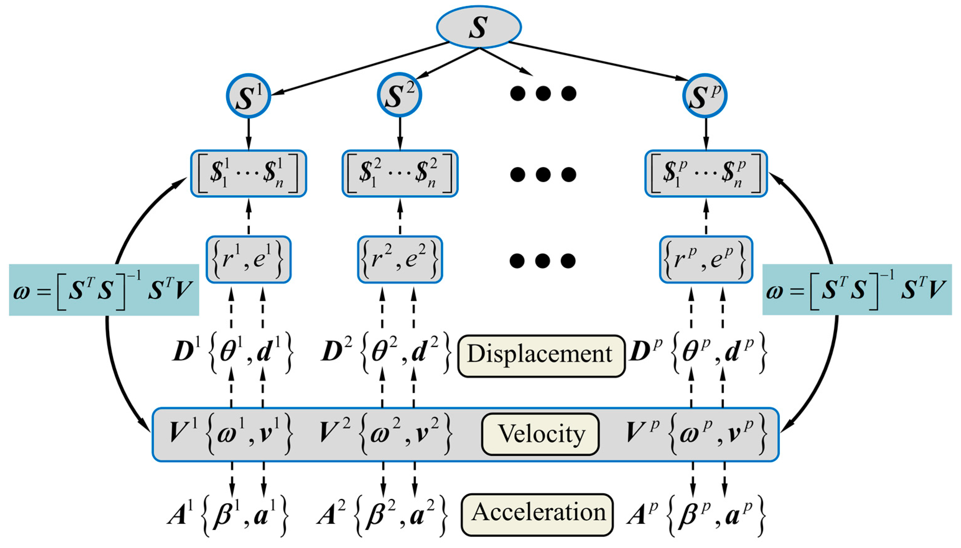
The absolute acceleration of a point on the rigid-body in the absolute ground coordinate frame 0 can be directly used in the Newton-Euler dynamics of a multi-rigid-body system. The procedures of the above calculation are illustrated in Figure 2.

Figure 2. The procedure for the kinematics on multi-rigid-body system.

3. Dynamics of a Multi-Rigid-Body System

The dynamics of a rigid body was described by the Newton–Euler equations in classical mechanics. Euler’s two laws of motion for a rigid body are grouped together into a single equation by the Newton–Euler equation. When the external loads, constraint forces, and self-weights of all bodies are taken into account in the calculation of wrenches, the balance conditions for a single-rigid-body will be

$$\left[\begin{array}{c}\mathit{T}\\ \mathit{F}\end{array}\right]=\left[\begin{array}{cc}{\mathit{J}}_n& 0\\ 0& m_n\mathit{I}\end{array}\right]\left[\begin{array}{c}\mathit{\beta }\\ \mathit{a}\end{array}\right]+\left[\begin{array}{c}\mathit{\omega }\times {\mathit{J}}_n\mathit{\omega }\\ m_n\mathbf{g}\end{array}\right]$$

(22)

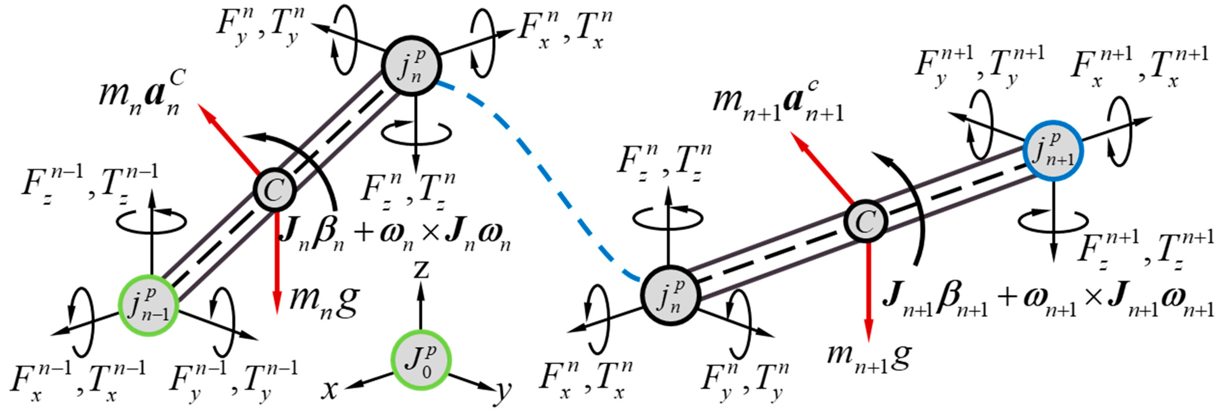
where $\mathit{T}={\mathit{T}}^n-{\mathit{T}}^{n-1}$ is the resultant torque of a single-rigid-body, in which ${\mathit{T}}^n$ is the constraint torque vector at joint $j_n$, $\mathit{F}={\mathit{F}}^n-{\mathit{F}}^{n-1}$ is the resultant force of a single-rigid-body, in which ${\mathit{F}}^n$ is the constraint force vector at joint $j_n$, $\mathit{I}$ is an identity matrix of $3\times 3$, $m_n$ is the mass of a single-rigid-body, $\mathit{a}$ is the absolute linear acceleration at the mass center, $\mathit{\beta }$ is the absolute angular acceleration, and $\mathit{\omega }$ is the absolute angular velocity. Figure 3 demonstrates the Newton-Euler parameters of two adjacent bodies in a multi-rigid-body system.

$${\mathit{J}}_0={\mathit{R}}_{0n}{\mathit{J}}_n{\mathit{R}}_{0n}^T$$

(23)

where ${\mathit{J}}_0$ is the matrix of mass moment of inertia of a single-rigid-body at its mass center in the absolute coordinate frame (coordinate frame 0), ${\mathit{J}}_n$ is the matrix of mass moment of inertia of a single-rigid-body at its principal coordinate frame of the mass center (coordinate frame $n$), and ${\mathit{R}}_{0n}$ is the rotation matrix from the coordinate frame $n$ to the coordinate frame 0.

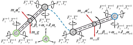
Figure 3. Newton-Euler parameters.

The Newton–Euler equations of dynamics of the multi-rigid-body system can be therefore be written as:

$$\mathit{C}{\mathit{W}}^S=\mathit{M}{\mathit{A}}^M+{\mathit{W}}^C+{\mathit{W}}^E$$

(24)

where ${\mathit{W}}^S={\left[\begin{array}{cccc}{\left[\begin{array}{c}{\mathit{T}}_1\\ {\mathit{F}}_1\end{array}\right]}^T& {\left[\begin{array}{c}{\mathit{T}}_2\\ {\mathit{F}}_2\end{array}\right]}^T& \cdots & {\left[\begin{array}{c}{\mathit{T}}_n\\ {\mathit{F}}_n\end{array}\right]}^T\end{array}\right]}^T$ is the constraint wrench matrix of a multi-rigid-body system including all constraint forces and constraint torques, ${\mathit{W}}^C$ is the Coriolis wrench matrix of the multi-rigid-body system, ${\mathit{W}}^E$ is the external wrench matrix exerted at the multi-rigid-body system which also includes the gravity, $\mathit{C}$ is the displacement matrix, $\mathit{M}$ is the mass matrix, and ${\mathit{A}}^M$ is the acceleration matrix composed by the absolute accelerations of the mass centers in the multi-rigid-body system.

When the number of constraint wrenches equals the number of equations in Equation (24), the supporting wrench can be calculated by

$${\mathit{W}}^S={\left(\mathit{C}{\mathit{C}}^T\right)}^{-1}\left(\mathit{M}{\mathit{A}}^M+{\mathit{W}}^C+{\mathit{W}}^E\right)$$

(25)

4. Kinematics and Dynamics of the Gough–Stewart Platform

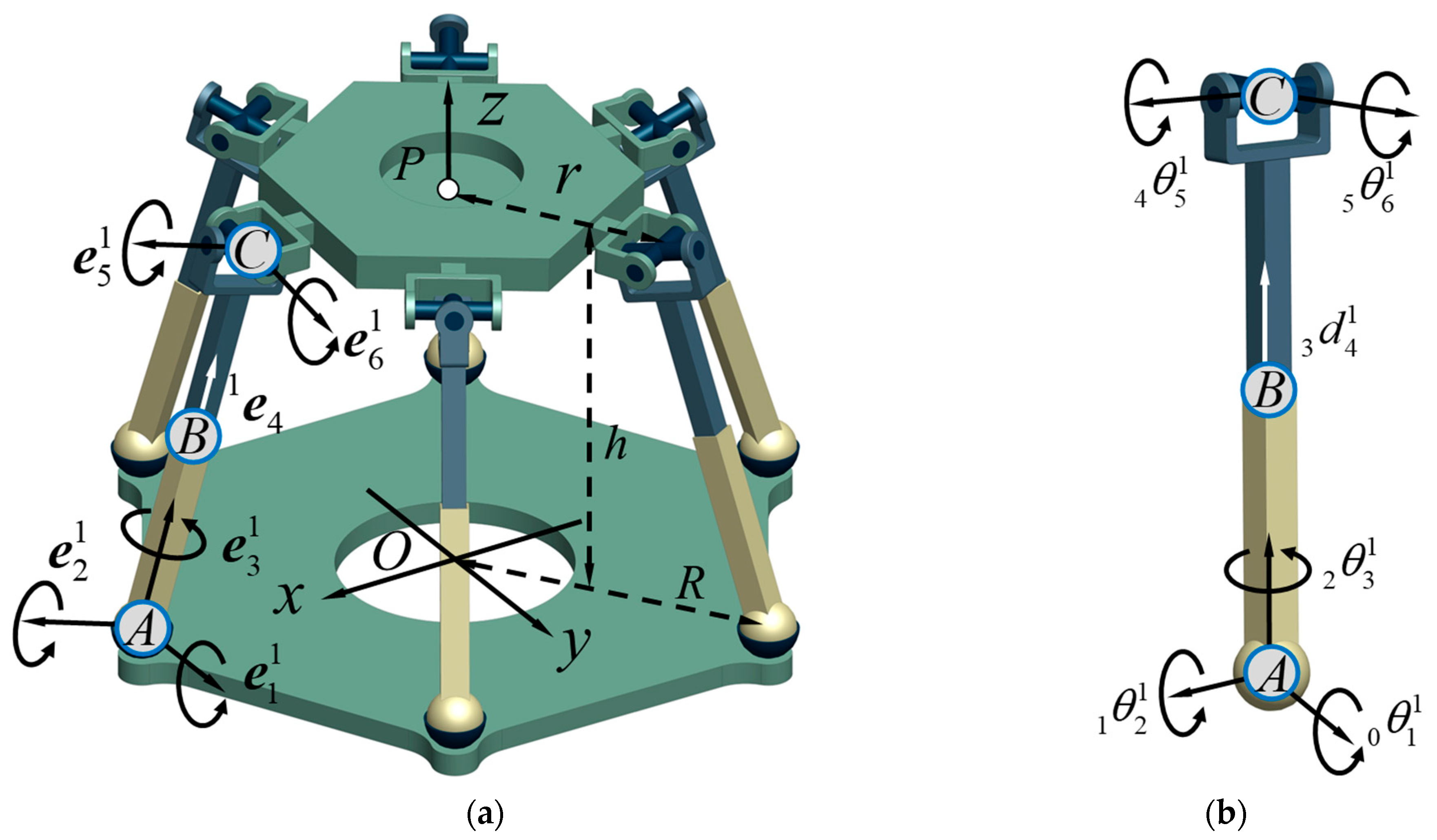
In this section, an application of the above method will be presented in the example of the Gough–Stewart platform. As shown in Figure 4, the Gough–Stewart platform consists of six kinematic chains, which are composed of a spherical joint, a prismatic joint and a universal joint. To simplify the expression of the kinematic chains, the spherical joint, prismatic joint, and universal joint are presented by the capital of the first letter of the joint name: $\mathrm{S}$, $\mathrm{P}$, and $\mathrm{U}$, respectively. The prismatic joint $\mathrm{P}$ is the actuated joint in the multi-rigid-body system. The Gough–Stewart platform has a fixed base and a moving manipulator connected by six extendable legs through universal joints at both ends.

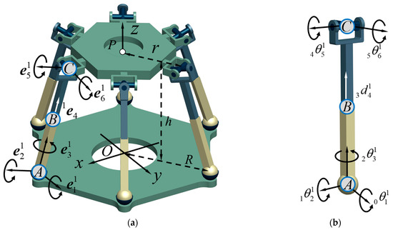
Figure 4. Kinematics analysis of the Gough–Stewart platform: (a) kinematics of the Gough–Stewart platform; (b) initial condition of the first kinematic chain.

4.1. Kinematics Analysis of the Gough–Stewart Platform

This section gives the inverse kinematics analysis of the Gough–Stewart platform. As shown in Figure 4, the inverse kinematics of the Gough–Stewart platform can be expressed as:

$$\mathit{S}\mathit{\omega }={\mathit{V}}_C$$

(26)

where $\mathit{S}=\mathit{diag}\left[\begin{array}{cccccc}{\mathit{S}}^1& {\mathit{S}}^2& {\mathit{S}}^3& {\mathit{S}}^4& {\mathit{S}}^5& {\mathit{S}}^6\end{array}\right]$ in which ${\mathit{S}}^p=\left[\begin{array}{cccccc}{\mathsf{\$}}_1^p& {\mathsf{\$}}_2^p& {\mathsf{\$}}_3^p& {\mathsf{\$}}_4^p& {\mathsf{\$}}_5^p& {\mathsf{\$}}_6^p\end{array}\right],$ and ${\mathsf{\$}}_1^p=\left[\begin{array}{c}{\mathit{e}}_1^p\\ {}_0\mathit{r}_A^p\times {\mathit{e}}_1^p\end{array}\right]$, ${\mathsf{\$}}_2^p=\left[\begin{array}{c}{\mathit{e}}_2^p\\ {}_0\mathit{r}_A^p\times {\mathit{e}}_2^p\end{array}\right]$, ${\mathsf{\$}}_3^p=\left[\begin{array}{c}{\mathit{e}}_3^p\\ {}_0\mathit{r}_A^p\times {\mathit{e}}_3^p\end{array}\right]$, ${\mathsf{\$}}_4^p=\left[\begin{array}{c}0\\ {\mathit{e}}_4^p\end{array}\right]$, ${\mathsf{\$}}_5^p=\left[\begin{array}{c}{\mathit{e}}_5^p\\ {}_0\mathit{r}_C^p\times {\mathit{e}}_5^p\end{array}\right]$, ${\mathsf{\$}}_6^p=\left[\begin{array}{c}{\mathit{e}}_6^p\\ {}_0\mathit{r}_C^p\times {\mathit{e}}_6^p\end{array}\right]$, $p=1,2,\cdots ,6$, $\mathit{\omega }={\left[\begin{array}{cccccc}{\mathit{\omega }}^1& {\mathit{\omega }}^2& {\mathit{\omega }}^3& {\mathit{\omega }}^4& {\mathit{\omega }}^5& {\mathit{\omega }}^6\end{array}\right]}^T$ and where ${\mathit{\omega }}^1={\left[\begin{array}{cccccc}{}_0\mathit{\omega }_1^1& {}_1\mathit{\omega }_2^1& {}_2\mathit{\omega }_3^1& {}_3\mathit{V}_4^1& {}_4\mathit{\omega }_5^1& {}_5\mathit{\omega }_6^1\end{array}\right]}^T$.

To get the unit screws in Equation (26), the rotation matrix is applied to express ${\mathit{e}}_n^p,{\mathit{r}}_n^p$ of each joint in the local coordinate frame, $p$ represents the $pth$ chain, and $n$ represents the $nth$ joint in a chain.

$$\{\begin{array}{l}{\mathit{e}}_n^p={\mathit{R}}_Z^p\left({\displaystyle \prod _{n=2}{\mathit{R}}_n^p}\right){\mathit{e}}_n^p\left(0\right)\\ {\mathit{r}}_n^p={\mathit{R}}_Z^p\left({}_0\mathit{r}_A^p\left(0\right)+{\mathit{R}}_2^p{\mathit{R}}_3^p{\mathit{R}}_5^p{\mathit{r}}_{AC}^p\right)\end{array},\{\begin{array}{c}\left(n=1,2,\cdots ,6\right)\\ \left(p=1,2,\cdots ,6\right)\end{array}$$

(27)

where ${\mathit{R}}_Z^p$ is the rotation matrix around z axis, which can be expressed as: ${\mathit{R}}_Z^p=R_z\left(\frac{\pi }{6}\left(p-1\right)\right)$. ${\mathit{R}}_n^p$ is the rotation matrix from link $L_n$ to link $L_{n-1}$, when it rotates around $x$-axis, ${\mathit{R}}_n^p=R_x\left({}_{n-1}\theta _n^p\right)$, when it rotates around $y$-axis, ${\mathit{R}}_n^p=R_y\left({}_{n-1}\theta _n^p\right)$, and when it rotates around $z$-axis, ${\mathit{R}}_n^p=R_z\left({}_{n-1}\theta _n^p\right)$. The initial condition parameters are illustrated in Table 1, and ${\mathbf{I}}_{\left(3\times 3\right)}$ is an identity matrix of $3\times 3$.

Table 1. Initial conditions and rotation matrix of Gough–Stewart platform.

Initial posture	${\mathit{e}}_1^1\left(0\right)$	${\mathit{e}}_2^1\left(0\right)$	${\mathit{e}}_3^1\left(0\right)$	${\mathit{e}}_4^1\left(0\right)$	${\mathit{e}}_5^1\left(0\right)$	${\mathit{e}}_6^1\left(0\right)$
	${\left[\begin{array}{ccc}0& 1& 0\end{array}\right]}^T$	${\left[\begin{array}{ccc}1& 0& 0\end{array}\right]}^T$	${\left[\begin{array}{ccc}0& 0& 1\end{array}\right]}^T$	${\left[\begin{array}{ccc}0& 0& 0\end{array}\right]}^T$	${\left[\begin{array}{ccc}1& 0& 0\end{array}\right]}^T$	${\left[\begin{array}{ccc}0& 1& 0\end{array}\right]}^T$
Initial position	${\mathit{r}}_A^1\left(0\right)$		${\mathit{r}}_B^1\left(0\right)$		${\mathit{r}}_C^1\left(0\right)$
	${\left[\begin{array}{ccc}R& 0& 0\end{array}\right]}^T$		${\left[\begin{array}{ccc}0& 0& L\end{array}\right]}^T$		${\left[\begin{array}{ccc}0& 0& 2L\end{array}\right]}^T$
Homogeneous transformation matrix	${\mathbf{R}}_1^p$	${\mathbf{R}}_2^p$	${\mathbf{R}}_3^p$	${\mathbf{R}}_4^p$	${\mathbf{R}}_5^p$	${\mathbf{R}}_6^p$
	$I$	$T_y\left({}_0\theta _1^p\right)$	$T_x\left({}_1\theta _2^p\right)$	$I$	$T_z\left({}_2\theta _3^p\right)$	$T_x\left({}_4\theta _5^p\right)$

After knowing the velocity screw of the moving platform at its mass center in the absolute coordinate frame, the relative angular velocity of each chain $L^p,\left(p=1,2\cdots 6\right)$ can be derived based on Equation (14):

$$\mathit{\omega }={\left[{\mathit{S}}^T\mathit{S}\right]}^{-1}\mathit{S}{\mathit{V}}_C^p$$

(28)

where ${\mathit{V}}_C^p,\left(p=1,2\cdots 6\right)$ is the velocity screw of joint $j_C$, which can be expressed as:

$${\mathit{V}}_C^p={\mathit{V}}_P-{}_C\mathit{V}_P^p$$

(29)

where ${\mathit{V}}_P$ is the velocity screw of the reference point $P$ on the moving platform, and it is given for the inverse kinematics. ${}_C\mathit{V}_P^p,\left(p=1,2\cdots 6\right)$ is the relative kinematics screw from joint $j_C^p,\left(p=1,2\cdots 6\right)$ to the reference point $P$ on the moving platform. It can be expressed as:

$${}_C\mathit{V}_P^p=\left[\begin{array}{c}0\\ {}_0\mathit{\omega }_C^p\times {}_0\mathit{r}_P^p\end{array}\right]$$

(30)

where ${}_0\mathit{\omega }_C^p,\left(p=1,2\cdots 6\right)$ is the absolute angular velocity of the moving platform, and ${}_0\mathit{r}_P^p,\left(p=1,2\cdots 6\right)$ is the absolute position vector of the reference point $P$ on the moving platform.

4.2. Dynamics Analysis of the Gough–Stewart Platform

a. 

Inverse dynamics equations for the fixed leg $L_{AB}^p,\left(p=1,2\cdots 6\right)$

The fixed leg $L_{AB}^p,\left(p=1,2\cdots 6\right)$ consists of one spherical joint and one prismatic joint, which is shown in Figure 5b. At spherical joint $j_A^p,\left(p=1,2\cdots 6\right)$, there are three forces ${\mathit{F}}_A$ without torque. At prismatic joint $j_B^p,\left(p=1,2\cdots 6\right)$, there are three forces ${\mathit{F}}_B$ and three torques ${\mathit{T}}_B$. The dynamics equations for the fixed leg $L_{AB}^p,\left(p=1,2\cdots 6\right)$ can be derived:

$$\left[\begin{array}{c}{}_A\mathit{r}_D\times {\mathit{F}}_A-{}_D\mathit{r}_B\times {\mathit{F}}_B-{\mathit{T}}_B\\ {\mathit{F}}_A-{\mathit{F}}_B\end{array}\right]=\left[\begin{array}{cc}{\mathit{J}}_D& 0\\ 0& m_D\mathbf{I}\end{array}\right]\left[\begin{array}{c}{\mathit{\beta }}_D\\ {\mathit{a}}_D\end{array}\right]+\left[\begin{array}{c}{\mathit{\omega }}_D\times {\mathit{J}}_D{\mathit{\omega }}_D\\ m_D\mathbf{g}\end{array}\right]$$

(31)

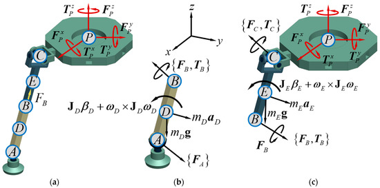
Figure 5. Dynamic analysis of the Gough–Stewart platform: (a) dynamics of the first kinematic chain; (b) dynamics of the fixed leg $L_{AB}^p,\left(p=1,2\cdots 6\right)$; (c) dynamics of the moving leg $L_{BC}^p,\left(p=1,2\cdots 6\right)$.

b. 

Inverse dynamics equations for the moving leg $L_{B\mathit{C}}^p,\left(p=1,2\cdots 6\right)$

The moving leg $L_{BC}^p,\left(p=1,2\cdots 6\right)$ consists of one universal joint and one prismatic joint which is shown in Figure 5c. At universal joint $j_C^p,\left(p=1,2\cdots 6\right)$, there are three forces ${\mathit{F}}_C$ and one torque ${\mathit{T}}_C$, the direction of the torque ${\mathit{T}}_C$ at joint $j_C^p,\left(p=1,2\cdots 6\right)$ is along the leg. At prismatic joint $j_B^p,\left(p=1,2\cdots 6\right)$, there are three forces ${\mathit{F}}_B$ and three torques ${\mathit{T}}_B$. The dynamics equations for the fixed leg $L_{BC}^p,\left(p=1,2\cdots 6\right)$ can be expressed by

$$\left[\begin{array}{c}{}_B\mathit{r}_E\times {\mathit{F}}_B-{}_E\mathit{r}_C\times {\mathit{F}}_C+{\mathit{T}}_B-{\mathit{T}}_C\\ {\mathit{F}}_B-{\mathit{F}}_C\end{array}\right]=\left[\begin{array}{cc}{\mathit{J}}_E& 0\\ 0& m_E\mathbf{I}\end{array}\right]\left[\begin{array}{c}{\mathit{\beta }}_E\\ {\mathit{a}}_E\end{array}\right]+\left[\begin{array}{c}{\mathit{\omega }}_E\times {\mathit{J}}_E{\mathit{\omega }}_E\\ m_E\mathbf{g}\end{array}\right]$$

(32)

c. 

Inverse dynamics equations for the moving platform $L_P$

The moving platform $L_P$ consists of six universal joints $j_C^p,\left(p=1,2\cdots 6\right)$, which are shown in Figure 5c. At the universal joint $j_C^p,\left(p=1,2\cdots 6\right)$, there are three forces ${\mathit{F}}_C$ and one torque ${\mathit{T}}_C$. Suppose that there is an external force system (if any) acting on the moving platform, which consists of a force ${\mathit{F}}_P$ and a torque ${\mathit{T}}_P$ in the absolute coordinate frame. The dynamics equations for the moving platform $L_P$ are expressed by

$$\left[\begin{array}{c}{\displaystyle \sum _{p=1}^6\left({}_0\mathit{r}_C\times {\mathit{F}}_C\right)+{\displaystyle \sum _{p=1}^6{\mathit{T}}_C}}\\ {\displaystyle \sum _{p=1}^6{\mathit{F}}_C}\end{array}\right]=\left[\begin{array}{cc}{\mathit{J}}_P& 0\\ 0& m_P\mathbf{I}\end{array}\right]\left[\begin{array}{c}{\mathit{\beta }}_P\\ {\mathit{a}}_P\end{array}\right]+\left[\begin{array}{c}{\mathit{\omega }}_P\times {\mathit{J}}_P{\mathit{\omega }}_P\\ m_P\mathbf{g}\end{array}\right]+\left[\begin{array}{c}{\mathit{T}}_P\\ {\mathit{F}}_P\end{array}\right]$$

(33)

d. 

Inverse dynamics equations for Gough–Stewart platform

Suppose,

$${\mathit{W}}^S=\left[\begin{array}{ccccc}{\mathit{F}}_A& {\mathit{F}}_B& {\mathit{F}}_C& {\mathit{T}}_B& {\mathit{T}}_C\end{array}\right]$$

(34)

where ${\mathit{F}}_A={\left[\begin{array}{cccc}{\mathit{F}}_A^1& {\mathit{F}}_A^2& \cdots & {\mathit{F}}_A^6\end{array}\right]}^T$, in which ${\mathit{F}}_A^1$ is the supporting force at joint $j_A^1$, and ${\mathit{F}}_A^1$ can be expressed by a 3-dimensional vector, and ${\mathit{T}}_B={\left[\begin{array}{cccc}{\mathit{T}}_B^1& {\mathit{T}}_B^2& \cdots & {\mathit{T}}_B^6\end{array}\right]}^T$, in which ${\mathit{T}}_B^1$ is the supporting torque at joint $j_B^1$, and ${\mathit{T}}_B^1$ can be expressed by a 3-dimensional vector.

Suppose,

$$\mathit{C}=\left[\begin{array}{ccccc}{}_A\hat{\mathit{r}}_D& -{}_D\hat{\mathit{r}}_B& {\mathbf{0}}_{\left(18\times 18\right)}& -{\mathbf{I}}_{\left(18\times 18\right)}& {\mathbf{0}}_{\left(18\times 6\right)}\\ {\mathbf{I}}_{\left(18\times 18\right)}& -{\mathbf{I}}_{\left(18\times 18\right)}& {\mathbf{0}}_{\left(18\times 18\right)}& {\mathbf{0}}_{\left(18\times 18\right)}& {\mathbf{0}}_{\left(18\times 6\right)}\\ {\mathbf{0}}_{\left(18\times 18\right)}& {}_B\hat{\mathit{r}}_E& -{}_E\hat{\mathit{r}}_C& {\mathbf{I}}_{\left(18\times 18\right)}& -{}_A\mathit{e}_{C\left(18\times 6\right)}\\ {\mathbf{0}}_{\left(18\times 18\right)}& {\mathbf{I}}_{\left(18\times 18\right)}& -{\mathbf{I}}_{\left(18\times 18\right)}& {\mathbf{0}}_{\left(18\times 18\right)}& {\mathbf{0}}_{\left(18\times 6\right)}\\ {\mathbf{0}}_{\left(3\times 18\right)}& {\mathbf{0}}_{\left(3\times 18\right)}& -{}_P\hat{\mathit{r}}_C& {\mathbf{0}}_{\left(3\times 18\right)}& -{}_A\mathit{e}_{C\left(3\times 6\right)}\\ {\mathbf{0}}_{\left(3\times 18\right)}& {\mathbf{0}}_{\left(3\times 18\right)}& -{\mathbf{I}}_{\left(3\times 18\right)}& {\mathbf{0}}_{\left(3\times 18\right)}& {\mathbf{0}}_{\left(3\times 6\right)}\end{array}\right]$$

(35)

where ${\mathbf{I}}_{\left(n\times n\right)}$ is an identity matrix of $n\times n$, ${\mathbf{I}}_{\left(3\times 18\right)}=\left[\begin{array}{cccccc}{\mathbf{I}}_{\left(3\times 3\right)}& {\mathbf{I}}_{\left(3\times 3\right)}& {\mathbf{I}}_{\left(3\times 3\right)}& {\mathbf{I}}_{\left(3\times 3\right)}& {\mathbf{I}}_{\left(3\times 3\right)}& {\mathbf{I}}_{\left(3\times 3\right)}\end{array}\right]$, and $0_{\left(n\times m\right)}$ is a zero-matrix. In Equation (30), $\hat{\mathit{r}}=\left[\begin{array}{ccc}0& -r_z& r_y\\ r_z& 0& -r_x\\ -r_y& r_x& 0\end{array}\right]$ and $\hat{\mathit{r}}$ is a skew matrix which consists of the position vector of joint $j_n^p,\left(p=1,2\cdots 6\right),\left(n=1,2\cdots 6\right)$ in the absolute coordinate frame.

Suppose,

$${\mathit{A}}^M={\left[\begin{array}{ccc}{\mathit{A}}_D& {\mathit{A}}_E& {\mathit{A}}_P\end{array}\right]}^T$$

(36)

where ${\mathit{A}}_D={\left[\begin{array}{cccc}{\left({\mathit{A}}_D^1\right)}^T& {\left({\mathit{A}}_D^2\right)}^T& \cdots & {\left({\mathit{A}}_D^6\right)}^T\end{array}\right]}^T$, in which ${\mathit{A}}_D^1=\left[\begin{array}{c}{\mathit{\beta }}_D^1\\ {\mathit{a}}_D^1\end{array}\right]$, and ${\mathit{A}}_D^1$ is the absolute acceleration of the mass center $D$ at the fixed leg $L_{AB}^1$ in the absolute coordinate frame.

Suppose,

$$\mathit{M}=\mathit{diag}\left[\begin{array}{ccc}{\mathit{M}}_D& {\mathit{M}}_E& {\mathit{M}}_P\end{array}\right]$$

(37)

where ${\mathit{M}}_D^1=\left[\begin{array}{cc}{\mathit{J}}_D^1& 0\\ 0& m_D^1\mathbf{I}\end{array}\right]$, and ${\mathit{M}}_D^1$ is the mass matrix consisting of ${\mathit{J}}_D^1$, the matrix of mass moment of inertia of the fixed leg $L_{AB}^1$, and mass $m_D^1$ which contains mass of the fixed leg $L_{AB}^1$.

Suppose,

$${\mathit{W}}^C={\left[\begin{array}{ccc}{\mathit{W}}_D& {\mathit{W}}_E& {\mathit{W}}_P\end{array}\right]}^T$$

(38)

where ${\mathit{W}}_D={\left[\begin{array}{cccc}{\left({\mathit{W}}_D^1\right)}^T& {\left({\mathit{W}}_D^2\right)}^T& \cdots & {\left({\mathit{W}}_D^6\right)}^T\end{array}\right]}^T$, in which ${\mathit{W}}_D^1=\left[\begin{array}{c}{\mathit{\omega }}_D^1\times {\mathit{J}}_D^1{\mathit{\omega }}_D^1\\ m_D^1\mathbf{g}\end{array}\right]$, and ${\mathit{W}}_D^1$ is a matrix consisting of the inertial torque resulting from Coriolis forces and the force of gravity.

Suppose,

$${\mathit{W}}^E=\left[\begin{array}{c}{\mathit{T}}_P\\ {\mathit{F}}_P\end{array}\right]=\left[\begin{array}{c}{\mathit{r}}_P\times {\mathit{F}}_P\\ {\mathit{F}}_P\end{array}\right]=\left[\begin{array}{c}{}_0\mathit{D}_P\left(4:6\right)\times {\mathit{F}}_P\\ {\mathit{F}}_P\end{array}\right]$$

(39)

where ${\mathit{W}}^E$ is the external force vector (if any) acting on the moving platform and is available as a force ${\mathit{F}}_P$ and a torque ${\mathit{T}}_P$ in the local coordinate frame of reference, and ${}_0\mathit{D}_P\left(4:6\right)$ represents the columns from 4 to 6 of matrix ${}_0\mathit{D}_P$.

Substituting Equations (34)–(39) into Equation (24), the dynamics equation of Gough–Stewart platform can be derived as:

$$\mathit{C}{\mathit{W}}^S=\mathit{M}{\mathit{A}}^M+{\mathit{W}}^C+{\mathit{W}}^E$$

(40)

When the number of constraint wrenches in Gough–Stewart platform is 78, and the sum of Equations (31)–(33) are 78, the wrenches can be calculated by Equation (40),

$${\mathit{W}}^S={\left(\mathit{C}{\mathit{C}}^T\right)}^{-1}\left(\mathit{M}{\mathit{A}}^M+{\mathit{W}}^C+{\mathit{W}}^E\right)$$

(41)

5. Numerical Experiment and Discussion

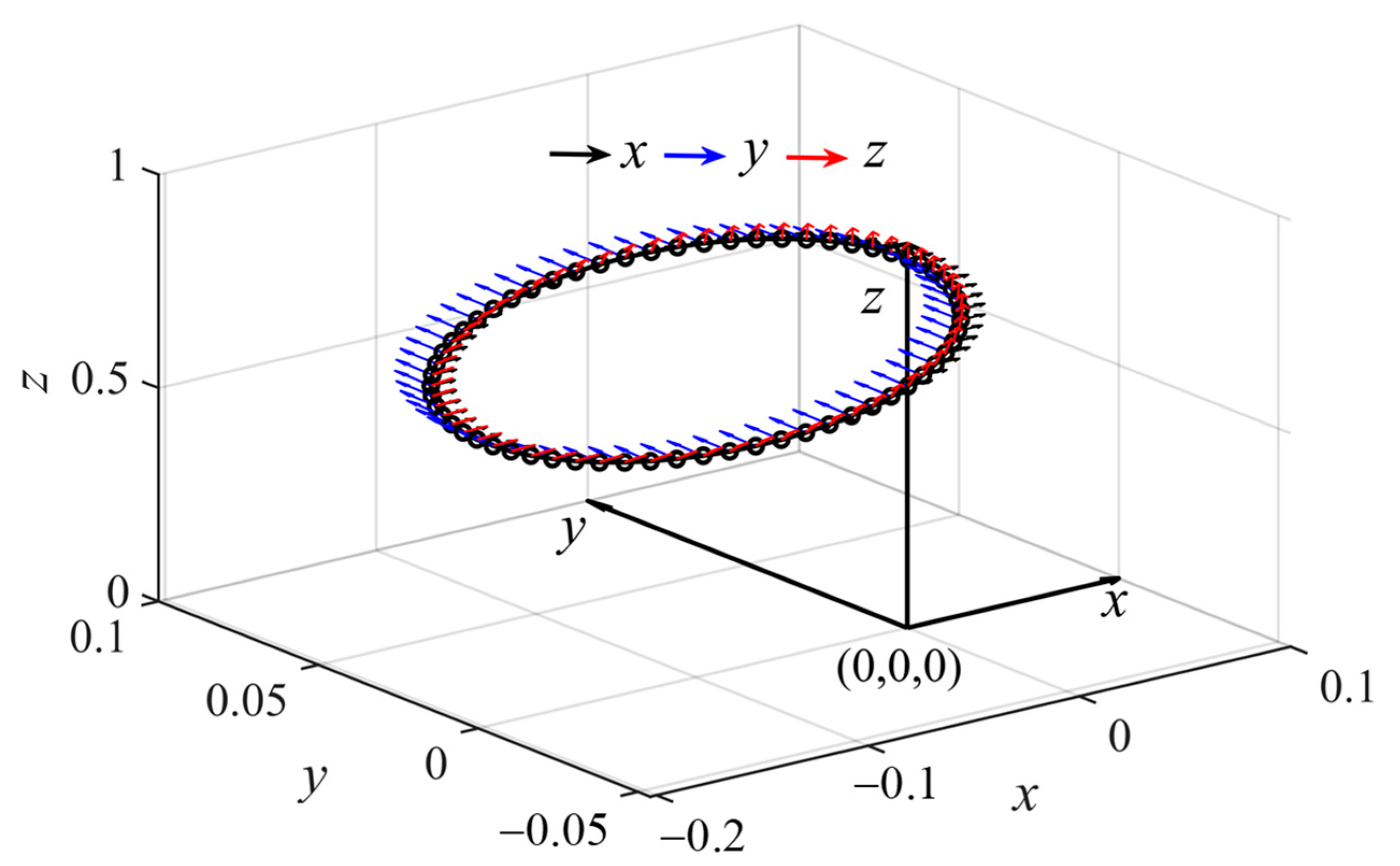
In this section, a prescribed trajectory is used to evaluate the inverse kinematics and dynamics of the Gough–Stewart platform. It has 6 degrees of freedom, including 3 translations and 3 rotations. Suppose that the moving platform follows a spiral trajectory. Here, the parametric equations of the path in displacement, velocity, and acceleration in the absolute coordinate frame are listed in Table A1. With the initial spiral trajectory of the moving platform in Figure 6, the inverse kinematics solutions of the Gough–Stewart platform can be applied directly to the dynamics.

Figure 6. Kinematics analysis of the Gough–Stewart platform.

5.1. Inverse Kinematics Simulation for Gough–Stewart Platform

When the velocity screw of the reference point $P$ on the moving platform is specified in Appendix A Table A1, and the initial conditions of the Gough–Stewart platform are also provided in Table A2 and Table A3, the inverse velocity and the inverse displacement (through one-step numerical integration) and acceleration (through one-step numerical differentiation) of the Gough–Stewart platform could be programmed in accordance with the algorithms deduced in Section 3. With the discrete conditions in Table 2 for the numerical calculations, the kinematics parameters can be output by programming in MATLAB. In Figure 7, Figure 8, Figure 9, Figure 10 and Figure 11, the kinematics of each kinematic chain for the Gough–Stewart platform are all plotted.

Table 2. Discrete conditions for numerical algorithm.

Initial Condition	Parameters	Value
Total time of the path	$t\left(s\right)$	$10$
Interval of iteration	$\Delta t$	$0.001$
Steps of iteration	$k$	$\mathrm{10,000}$

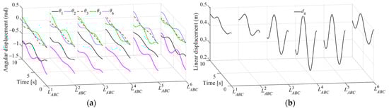
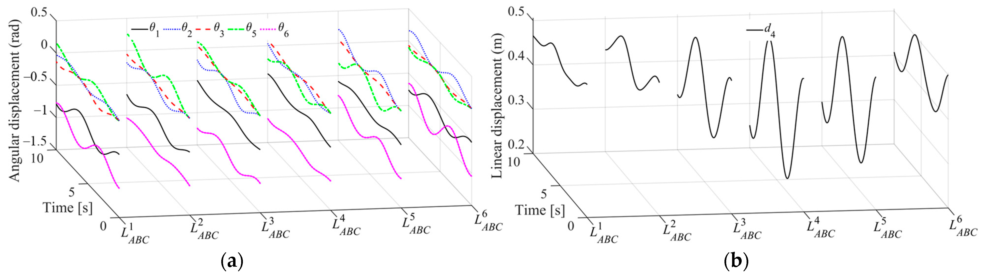
Figure 7. Relative displacements of the joints in each link: (a) relative angular displacements; (b) relative linear displacements.

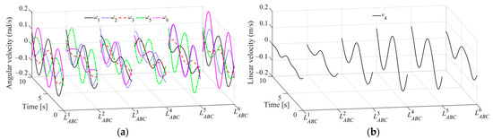
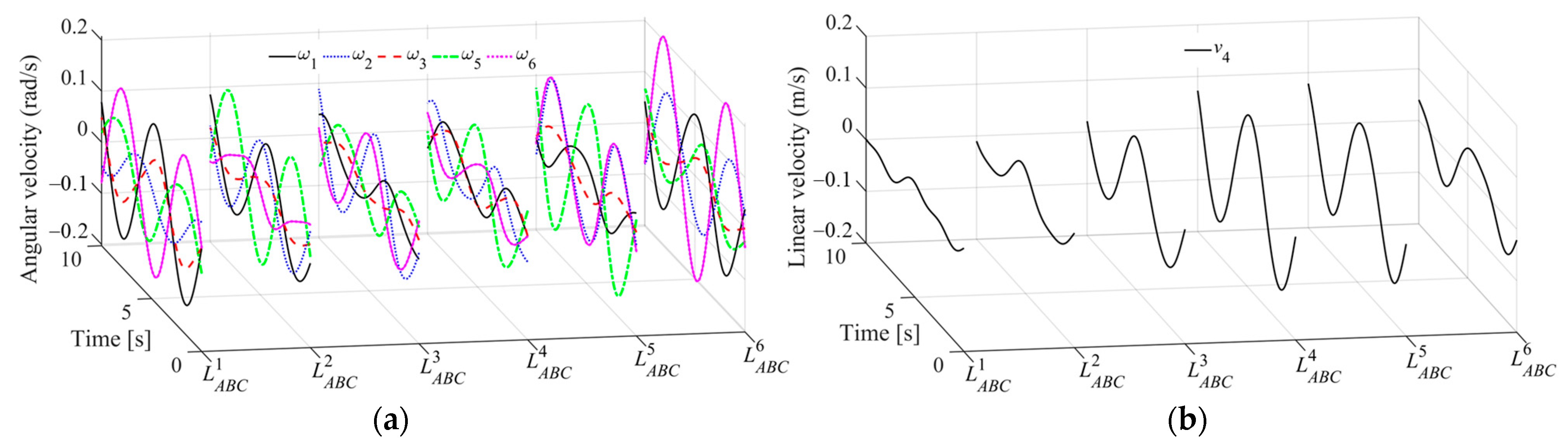
Figure 8. Relative velocities of each joint in each link: (a) relative angular velocities; (b) relative linear velocities.

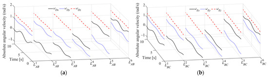
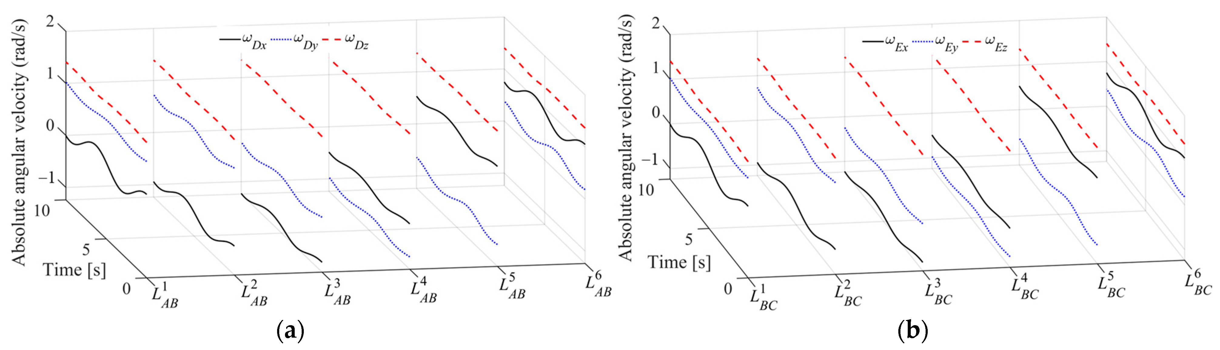
Figure 9. Absolute angular velocities of all legs: (a) absolute angular velocities of the fixed legs $L_{AB}^p,\left(p=1,2\cdots 6\right)$; (b) absolute angular velocities of the moving legs $L_{BC}^p,\left(p=1,2\cdots 6\right)$.

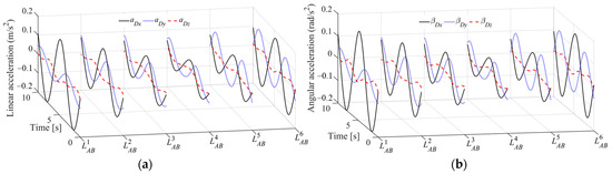
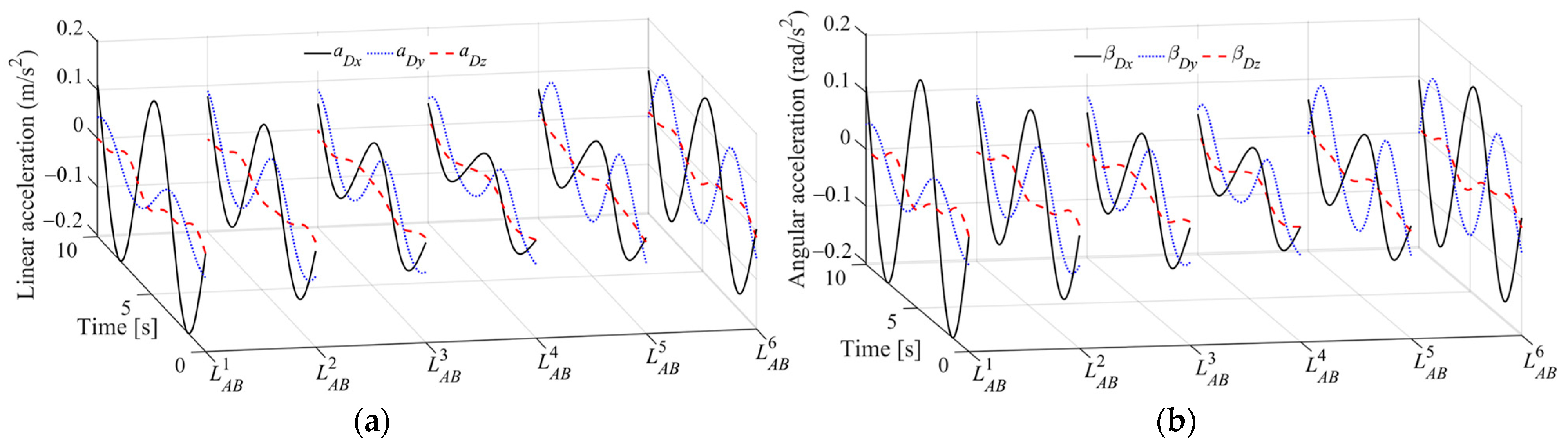
Figure 10. Absolute accelerations of the fixed legs $L_{AB}^p,\left(p=1,2\cdots 6\right)$ at their individual mass centers: (a) absolute linear accelerations of the mass centers of the fixed legs; (b) absolute angular accelerations of the fixed legs.

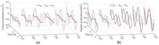
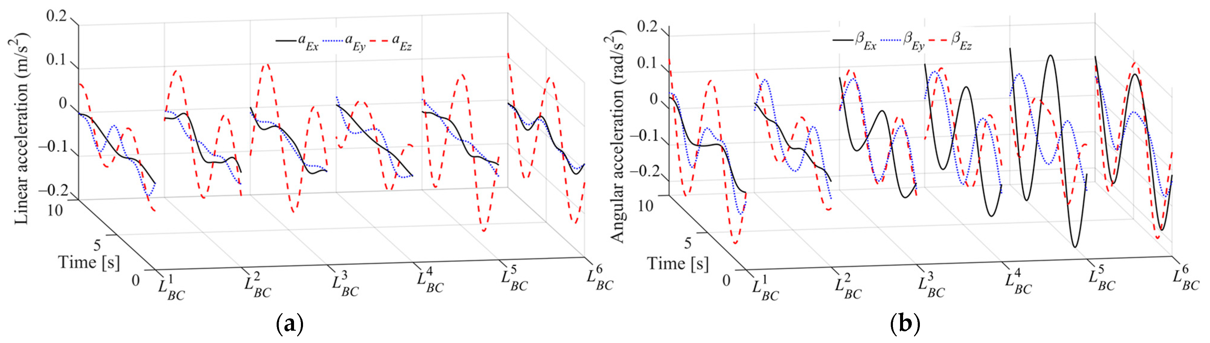
Figure 11. Absolute accelerations of the moving legs $L_{BC}^p,\left(p=1,2\cdots 6\right)$ at their respective mass centers: (a) absolute linear accelerations of the mass centers of the moving legs; (b) absolute angular accelerations of the moving legs.

Figure 7 illustrates the relative displacements of all joints. Figure 7a shows the angular displacements of all rotational joints, and Figure 7b represents the angular displacement of all prismatic joints. They are all solved by Equation (15) with the one-step numerical algorithm.

Figure 8 illustrates the relative velocities of all joints. Figure 8a shows the angular velocities of rotational joints, and Figure 8b shows the angular velocities of prismatic joints. They are all represented by Equation (14) with the one-step numerical algorithm.

Figure 9 illustrates the absolute angular velocities of all legs. Figure 9a shows the absolute angular velocities of the fixed legs $L_{AB}^p,\left(p=1,2\cdots 6\right)$, and Figure 9b shows the absolute angular velocities of the moving legs $L_{BC}^p,\left(p=1,2\cdots 6\right)$.

Figure 10 illustrates the absolute accelerations of the fixed legs $L_{AB}^p,\left(p=1,2\cdots 6\right)$ at their individual mass centers. Figure 10a shows the absolute linear accelerations of point $D$ on the fixed legs while Figure 10b illustrates the absolute angular accelerations.

Figure 11 illustrates the absolute accelerations of the moving legs $L_{BC}^p,\left(p=1,2\cdots 6\right)$ at their individual mass centers. Figure 11a shows the absolute linear accelerations of the mass centers of the moving legs, and Figure 11b shows the absolute angular accelerations of the moving legs.

5.2. Inverse Dynamics Simulation for Gough–Stewart Platform

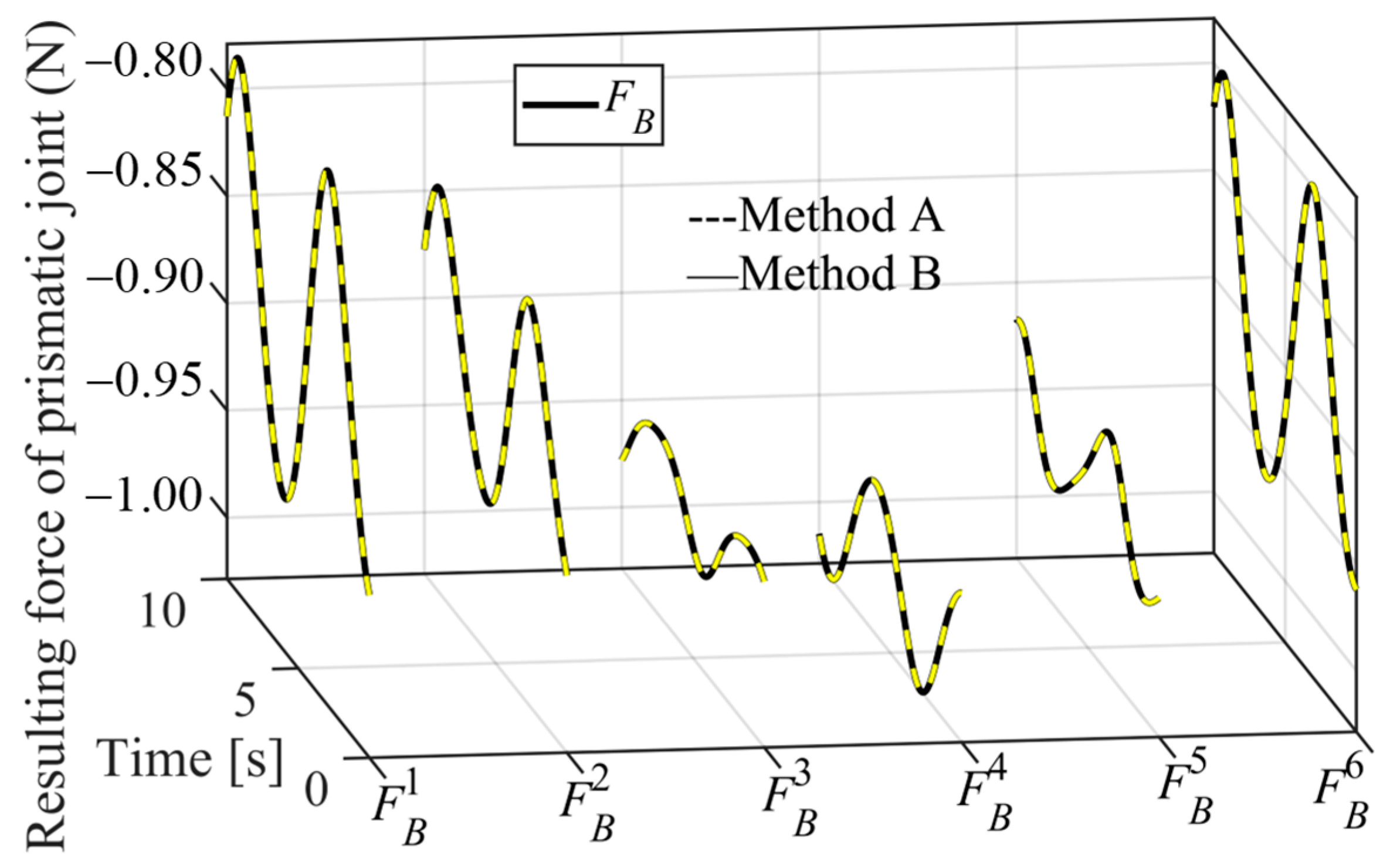
Suppose that the external force exerted on the moving platform at its center point $P$ is ${\mathit{F}}_P=\left[\begin{array}{ccc}0& 0& 10\end{array}\right]\left(N\right)$, and the torque is ${\mathit{M}}_P=\left[\begin{array}{ccc}10& 0& 0\end{array}\right]\left(Nm\right)$. With the structure variables, the mass and the mass moment of inertia of each leg of the Gough–Stewart platform listed in Table A4 and the external force and torque applied on the moving platform, the forces and torques of the driving forces ${\mathit{F}}_B^p,\left(p=1,2,\cdots ,6\right)$ can be gained (Figure 12) from the dynamics Equation (41). In order to verify this method, we compare the output calculated by vector method and our method. In Figure 12, Method A illustrates the method this paper proposed and Method B presents the method proposed by Dasgupta [11,12].

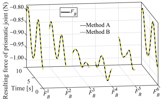
Figure 12. Resultant driving force of each prismatic joint $j_B^p,\left(p=1,2,\cdots ,6\right)$.

Figure 12 shows that the resultant driving forces at prismatic joint $j_B^p,\left(p=1,2,\cdots ,6\right)$ of the six kinematic chains. In addition, the component forces along the three coordinate frames can be derived from the direction of each chain, and the curves indicate that the driving forces are changing as the moving platform changes.

6. Conclusions

This paper provides a programmable method to solve the kinematics and dynamics of multi-rigid-body systems in screw coordinate. With this method, both displacement and acceleration are uniformly expressed in the matrix form of velocity, and as a result, a one-step numerical algorithm is sufficient to solve them for establishing the dynamics of a multi-rigid-body system. All constraint and driving forces and torques of the multi-rigid-body system can therefore be resolved straightforwardly in the form of screw coordinate. The kinematics and dynamics of the Gough–Stewart platform validate this method which is also suited to analyze a series of multi-rigid-body systems.

References

- Gough, V.E.; Whitehall, S.G. Proceedings of the 9th International Congress FISITA, London, UK, 30 April–5 May 1962.
- Fichter, E.F.; Kerr, D.R.; Rees-Jones, J. The Gough-Stewart platform parallel manipulator: A retrospective appreciation. Proc. Inst. Mech. Eng. 2009, 223, 243–281. [Google Scholar] [CrossRef]
- Furqan, M.; Suhaib, M.; Ahmad, N. Studies on Stewart platform manipulator: A review. J. Mech. Sci. Technol. 2017, 31, 4459–4470. [Google Scholar] [CrossRef]
- Hernández-Vielma, C.; Ortega-Aguilera, R.; Cruchaga, M. Assessment of simultaneous and nested conservative augmented Lagrangian schemes for constrained multibody dynamics. Proc. Inst. Mech. Eng. Part K J. Multi-Body Dyn. 2021, 235, 271–280. [Google Scholar] [CrossRef]
- Chen, M.; Zhang, Q.; Qin, X.; Sun, Y. Kinematic, dynamic, and performance analysis of a new 3-DoF over-constrained parallel mechanism without parasitic motion. Mech. Mach. Theory 2021, 162, 104365. [Google Scholar] [CrossRef]
- Smith, A.; Yang, C.; Li, C.; Ma, H.; Zhao, L. Development of a dynamics model for the Baxter robot. In Proceedings of the International Conference on Mechatronics and Automation, Harbin, China, 7–10 August 2016; pp. 1244–1249. [Google Scholar]
- Gallardo-Alvarado, J.; Rodríguez-Castro, R.; Delossantos-Lara, P.J. Kinematics and dynamics of a 4-P RUR Schönflies parallel manipulator by means of screw theory and the principle of virtual work. Mech. Mach. Theory 2018, 122, 347–360. [Google Scholar] [CrossRef]
- Azad, F.A.; Yazdi, M.R.H.; Masouleh, M.T. Kinematic and Dynamic Analysis of 3-DOF Delta Parallel Robot Based on the Screw Theory and Principle of Virtual Work. In Proceedings of the 5th Conference on Knowledge Based Engineering and Innovation (KBEI), Tehran, Iran, 28 February–1 March 2019; pp. 717–724. [Google Scholar]
- Wen, S.; Qin, G.; Zhang, B.; Lam, H.; Zhao, Y.; Wang, H. The study of model predictive control algorithm based on the force/position control scheme of the 5-DoF redundant actuation parallel robot. Rob. Auton. Syst. 2016, 79, 12–25. [Google Scholar] [CrossRef]
- Mata, V.; Provenzano, S.; Cuadrado, J.L.; Valero, F. Inverse dynamic problem in robots using Gibbs-Appell equations. Robotica 2002, 20, 59–67. [Google Scholar] [CrossRef]
- Dasgupta, B.; Choudhury, P. A Newton-Euler formulation for the inverse dynamics of the Stewart platform manipulator. Mech. Mach. Theory 1998, 33, 1135–1152. [Google Scholar] [CrossRef]
- Dasgupta, B.; Mruthyunjaya, T.S. Closed-Form Dynamic Equations of the General Stewart Platform through the Newton–Euler Approach. Mech. Mach. Theory 1998, 33, 993–1012. [Google Scholar] [CrossRef]
- Chen, G.; Yu, W.; Li, Q.; Wang, H. Dynamic modeling and performance analysis of the 3-PRRU 1T2R parallel manipulator without parasitic motion. Nonlinear Dyn. 2017, 90, 339–353. [Google Scholar] [CrossRef]
- Wang, Z.; Zhao, D.; Zeng, G. The dynamic model of a 6-DOF parallel mechanism. Mach. Des. Manufact. 2018, S1, 71–77. [Google Scholar]
- Niu, A.; Wang, S.; Sun, Y.; Qiu, J.; Qiu, W.; Chen, H. Dynamic modeling and analysis of a novel offshore gangway with 3UPU/UP-RRP series-parallel hybrid structure. Ocean. Eng. 2022, 266, 113122. [Google Scholar] [CrossRef]
- Gallardo-Alvarado, J.; Aguilar-Nájera, C.R.; Casique-Rosas, L.; Pérez-González, L.; Rico-Martínez, J.M. Solving the kinematics and dynamics of a modular spatial hyper-redundant manipulator by means of screw coordinate. Multibody Syst. Dyn. 2008, 20, 307–325. [Google Scholar] [CrossRef]
- Gallardo-Alvarado, J.; Aguilar-Nájera, C.R.; Casique-Rosas, L.; Rico-Martínez, J.M.; Islam, M.N. Kinematics and dynamics of 2(3-RPS) manipulators by means of screw coordinate and the principle of virtual work. Mech. Mach. Theory 2008, 43, 1281–1294. [Google Scholar] [CrossRef]
- Tian, Q.; Xiao, Q.; Sun, Y.; Hu, H.; Liu, H.; Flores, P. Coupling dynamics of a geared multibody system supported by ElastoHydroDynamic lubricated cylindrical joints. Multibody Syst. Dyn. 2015, 33, 259–284. [Google Scholar] [CrossRef]
- Shan, X.; Gang, C. Nonlinear dynamic behavior of joint effects on a 2(3PUS + S) parallel manipulator. Proc. Inst. Mech. Eng. Part K J. Multi Body Dyn. 2018, 233, 470–484. [Google Scholar]
- Asadi, F.; Heydari, A. Analytical dynamic modeling of Delta robot with experimental verification. Proc. Inst. Mech. Eng. Part K J. Multi-Body Dyn. 2020, 234, 623–630. [Google Scholar] [CrossRef]
- Liu, C.; Tian, Q.; Hu, H.Y. Dynamics of a large scale rigid–flexible multibody system composed of composite laminated plates. Multibody Syst. Dyn. 2011, 26, 283–305. [Google Scholar] [CrossRef]
- Gan, D.; Dai, J.S.; Dias, J.; Seneviratne, L. Forward kinematics solution distribution and analytic singularity-free workspace of linear-actuated symmetrical spherical parallel manipulators. J. Mech. Robot. 2015, 7, 041007. [Google Scholar] [CrossRef]
- Dai, J.S.; Jones, J.R. A linear algebraic procedure in obtaining reciprocal screw systems. J. Robot. Syst. 2003, 20, 401–412. [Google Scholar] [CrossRef]
- Hashemi, E.; Khajepour, A. Kinematic and three-dimensional dynamic modeling of a biped robot. Proc. Inst. Mech. Eng. Part K J. Multi-Body Dyn. 2017, 231, 57–73. [Google Scholar] [CrossRef]
- Shen, H.; Chablat, D.; Zeng, B.; Li, J.; Wu, G.; Yang, T.L. A translational three-degrees-of-freedom parallel mechanism with partial motion decoupling and analytic direct kinematics. J. Mech. Robot. 2020, 12, 021112. [Google Scholar] [CrossRef]
- Kanaan, D.; Wenger, P.; Chablat, D. Kinematic analysis of a serial-parallel machine tool: The VERNE machine–Science Direct. Mech. Mach. Theory 2009, 44, 478–498. [Google Scholar] [CrossRef]
- Zhao, J.S.; Wei, S.T.; Ji, J.J. Kinematics of a planar slider-crank linkage in Plücker Coordinate. Proc. Inst. Mech. Eng. Part C J. Mech. Eng. Sci. 2022, 236, 1588–1597. [Google Scholar] [CrossRef]
- Gallardo-Alvarado, J.; Rico-Martinez, J.M. Kinematics of a hyper-redundant manipulator by means of screw coordinate. Proc. Inst. Mech. Eng. Part K J. Multi-Body Dyn. 2009, 223, 325–334. [Google Scholar]
Disclaimer/Publisher’s Note: The statements, opinions and data contained in all publications are solely those of the individual author(s) and contributor(s) and not of MDPI and/or the editor(s). MDPI and/or the editor(s) disclaim responsibility for any injury to people or property resulting from any ideas, methods, instructions or products referred to in the content. |
© 2023 by the authors. Licensee MDPI, Basel, Switzerland. This article is an open access article distributed under the terms and conditions of the Creative Commons Attribution (CC BY) license (https://creativecommons.org/licenses/by/4.0/).