Abstract
To comprehensively evaluate the seismic performance of offshore bridges, a seismic risk analysis of an example bridge was developed based on improved two-dimensional (2D) seismic fragility analysis. Taking a simply-supported beam bridge in an offshore tidal environment as an example, the adverse effects of chloride ion erosion are considered and the seismic response process of the example bridge is simulated using the Incremental Dynamic Analysis (IDA) method. The appropriate damage indexes are chosen for the plate rubber bearing and the pier, and the one-dimensional (1D) seismic fragility curves of single components and the entire bridge are obtained. The correlation coefficients of vulnerable components are quantitatively proposed based on the correlation analysis method, and the 2D seismic fragility curves of the entire bridge are achieved while accounting for seismic correlation between vulnerable components. The seismic risk probability of the entire bridge is finally determined after combining hazard analysis at the bridge site and seismic loss analysis. The results show that there is a significant correlation between vulnerable components and that 2D seismic fragility analysis based on the reliable correlation coefficients of vulnerable components can more comprehensively evaluate the seismic performance of the entire bridge. In the context of seismic disaster reduction research focused on slight and moderate damage caused by moderate-to-small ground motions, this research can provide scientific and technical support for seismic design and seismic risk assessment of offshore bridges.
1. Introduction
Bridges a vital component of road engineering infrastructure, and undertake such important functions as traffic and transportation. With the growing economic prosperity of coastal areas, offshore bridge construction has entered a period of rapid development. However, when offshore bridges have been in the marine environment for a long time, the chloride ion corrosion phenomenon can become severe. Corrosion of the reinforced concrete structure can have a wide range of adverse effects on the seismic performance of both single components and the entire bridge [1,2,3]. In addition, bridges can suffer large dynamic vibrations when ground motion occurs; in such cases, the seismic damage to single components and the entire bridge can be considerable, resulting in significant social and economic loss [3]. Therefore, it is critical to thoroughly conduct extensive seismic disaster risk research on offshore bridges and to ensure that rational seismic performance assessment considers chloride ion erosion.
Seismic risk analysis is mainly used to quantitatively analyze and evaluate the possibility of ground motions of varying intensities, as well as the potential loss caused by engineering buildings in potential risk areas. Seismic risk analysis of bridge engineering first began in the 1980s. With the introduction of performance seismic design concepts in recent years [4], domestic and foreign scholars have performed related research work on site hazard analysis, structural fragility analysis, and seismic loss analysis, yielding a great number of research findings. Mackie and Stojadinović directly defined the bridge structure’s damage level with the damage state of the pier while taking into account the uncertainty of seismic demand, and performed seismic risk analysis for an example bridge [5]. Padgett et al. conducted seismic risk and economic loss estimates for 375 bridges in South Carolina, United States, while accounting for uncertainty, providing a specific reference basis for determining bridge reinforcement plans and emergency response [6]. Kameshwar et al. proposed a multi-hazard risk assessment method based on parametric vulnerability, which is primarily applicable to highway bridge risk assessment under hurricane and earthquake actions [7]. Based on the IDA method, Feng et al. converted the seismic intensity at the bridge site into the corresponding peak ground acceleration using Monte Carlo sampling; a cable-stayed bridge was chosen as the research object to validate the accuracy of above-mentioned method, then seismic risk analysis was performed on it [8]. Han et al. took a high-speed railway continuous beam bridge as an example to establish a seismic demand model for bridge components using the strip method, followed by the development of a seismic vulnerability function for bridge components [9]. Combining the geological structural conditions of the project site and historical earthquake damage data, they conducted seismic risk assessment for an example bridge. Employing a high-speed railway continuous beam bridge as an example, Xiang et al. investigated the influence of bond slip and chloride ion erosion on the seismic fragility of the bridge; their results revealed that the seismic damage risk of components increased with the increase in the reinforcement corrosion rate [10]. Feng took a three-span continuous beam bridge as an example to calculate the seismic risk probability of an example bridge without taking into account time-varying characteristics [11].
The above excellent papers have greatly aided the research process of seismic risk analysis for bridge engineering. Furthermore, Wu and Li have proposed that the accurate seismic fragility analysis of the entire bridge, rather than of single components, is the essential premise of seismic risk analysis [12]. Therefore, relevant scholars have conducted extensive research and proposed several seismic fragility analysis methods for entire bridges, including the wide bound method [13], the Monte Carlo sampling method [14], and the multivariate copula function [15]. However, most studies have only considered the correlation between the seismic responses of different components, while ignoring the correlations between their seismic capacities. In view of this, Cimellaro et al. proposed multi-dimensional fragility analysis (MFA) based on multiple evaluation indexes in order to consider the correlation between the seismic capacity of different components, which has been widely applied to large structures [16]. Wang et al. applied MFA to the seismic performance evaluation of large-scale bridges based on the displacement of bridge bearings and the ductility ratio of the bridge pier, considering the uncertainty of both ground motions and structural performance limit states [17]. Xiang et al. applied MFA to seismic performance evaluation of large multi-tower structures based on the probability density evolution method [18]. According to the fundamental theory of MFA, a reasonable internal relationship of different indexes is a primary basis for fragility analysis [16]. However, most current papers only provide a qualitative value to represent the relationships between vulnerable components, and do not reveal the internal correlation mechanism to obtain rational correlation coefficients [17,19]. Therefore, the internal correlation mechanism between vulnerable components must be clarified, and the correlation coefficients under different seismic performance limit states should be further developed to propose an improved MFA. In this paper, we employ the improved MFA to achieve an accurate seismic risk analysis of an offshore bridge while taking into account chloride ion erosion and the seismic correlations between vulnerable components.
In this paper, a reinforced concrete simply-supported beam bridge in an offshore tidal environment is employed as an example. Considering the adverse effects of chloride ion erosion and the uncertainty of both structural material parameters and ground motions, we first establish 300 bridge–ground motion analysis sample pairs. The seismic response process of the example bridge is simulated employing the IDA method, with the plate rubber bearing and the pier selected as vulnerable components. Based on linear regression analysis and first-order reliability theory, 1D seismic fragility curves are obtained for both single components and the entire bridge. The internal relationship mechanism between the seismic demand and the seismic capacity of different components is further explored in order to clarify the correlation coefficients of the vulnerable components and obtain the 2D seismic fragility curves of the entire bridge while considering the seismic correlations between vulnerable components. The seismic risk probability of the entire bridge is further determined based on discrete conditional probability in combination with hazard analysis at the bridge site and seismic loss analysis. This research can provide scientific and technical support for seismic design and seismic risk assessment of offshore bridges. The flowchart of this paper is shown in Figure 1.
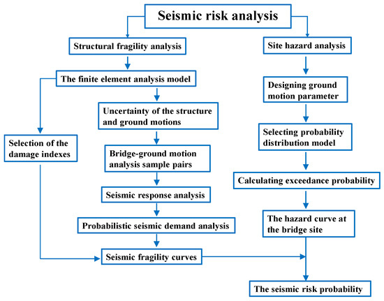
Figure 1.
Flowchart of the seismic risk analysis method used in this paper.
2. Example Bridge
2.1. Introduction of the Example Bridge
Prestressing as a means of connecting structural components promotes the development of innovative systems and construction methods for large-span structures. In this paper, a prestressed concrete simply-supported beam bridge with a span of 3 × 30 m in the offshore tidal environment is used as an example. As shown in Figure 2, the example bridge has been in service for 40 years and is located in a Class II site. The main structure adopts concrete of C40 grade with four T-beams arranged toward the transverse bridge. The height of the beam is 2.0 m, the total width of the bridge deck is 8.0 m, the capping beam adopts concrete of C30 grade, its length is 8 m, and its cross-section size is 1.5 m × 1.5 m. The pier is a double-column solid circular section pier of 1.5 m diameter and 10.5 m height; its water-cement ratio is 0.4, the longitudinal bars and stirrups are HRB335 steel bars, and the longitudinal reinforcement diameter is 25 mm; 26 pieces are arranged along the circular sections of piers; the stirrup diameter is 10 mm; and their spacing is 0.05 m in the form of spiral reinforcement. The concrete protection layer is 60 mm, with the abutments on both sides consisting of ribbed slab abutments with an expansion joint width of 50 mm between the abutment and the main beam. An ordinary rectangular plate rubber bearing (PETB) is used at the pier capping beam, with the total thickness of the rubber layer 50 mm. The schematic of the example bridge is shown in Figure 3.
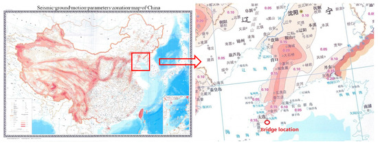
Figure 2.
Location of the example bridge.
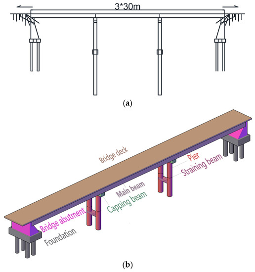
Figure 3.
Schematic of the example bridge: (a) elevation diagram and (b) structural drawing.
2.2. The Finite Element Analysis Model
The finite element analysis model of the entire bridge was established using OpenSees. Considering the advantages of no or fewer cracks in prestressed concrete structures, as well as similar engineering damage experience from previous earthquakes, the main beam would not undergo plastic deformation and the capping beam is always designed to be the capacity protection component. Therefore, the Elastic Beam Column Element was employed for the main beam and capping beam. The Zero Length Element was employed for bearings. The Force-Based Beam Column Element was employed for piers. The Mander model was used for the confined concrete in the bridge and the bilinear constitutive model was used for reinforcement, as shown in Figure 4. The concrete and reinforcement were defined by Concrete 04 Element and Steel 02 Element, respectively. According to the Seismic Design Criteria for Highway Bridges and Culverts [20], the expansion joints were simulated by the Elastic–Perfectly Plastic Gap Material. For simplicity, the interaction between the pile–soil structure is ignored in this paper. When the seismic P wave propagates in the sea, the cancellation interference effect greatly reduces the intensity of the vertical component of the seabed ground motion, resulting in a lower vertical and horizontal peak acceleration ratio of the seabed ground motion compared to that of the land ground motions. Therefore, the vertical ground motion is not considered in this paper [21,22,23].
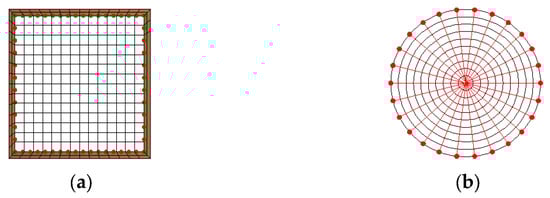
Figure 4.
Division of the cap beam and pier section: (a) cap beam and (b) pier.
2.3. Uncertainty of the Structural Parameters Considering Chloride Ion Erosion
2.3.1. Chloride Ion Erosion
The example bridge is located in an offshore tidal environment and is prone to corrosion degradation caused by chloride ion erosion. The chloride ion erosion process consists of three steps [24]: (1) diffusion, in which chloride ions diffuse to the reinforcement surface through the concrete protective layer until the reinforcement begins to corrode; (2) corrosion, in which the reinforcement corrodes and then the concrete cover begins to crack; and (3) degeneration, in which cracks occur in the concrete cover. The corrosion caused by chloride ion erosion has a negative impact on the overall seismic performance of the entire bridge. Therefore, the element model with consideration of chloride ion erosion should be employed to calculate the precise structural parameters of the example bridge at the current service time. The process of chloride ion corrosion in reinforced concrete structures is shown in Figure 5.
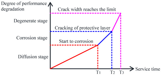
Figure 5.
The process of chloride ion corrosion in reinforced concrete structures.
- (1)
- Diffusion Stage
In this paper, the corrosion process of chloride ions to the interior of the pier concrete is simulated by employing Fick’s second diffusion law [25]. To begin, the corrosion is considered with continuous diffusion when the chloride ion concentration on the outer surface of the reinforcement reaches a threshold. The corrosion starting time () can be calculated by employing the following formulas [26]:
where is the thickness of the concrete cover, is the diffusion coefficient, is the inverse function of the Gaussian error, is the threshold for the chloride ion concentration, is the concentration of chloride ions on the concrete surface, is the water–cement ratio, and and are the calculation parameters. Previous papers have demonstrated that the parameters , , , are approximately subject to normal distributions; the statistical results are shown in Table 1 [27,28,29]. Here, is calculated as 19.40 years by taking the respective mean values and substituting the relevant parameters of the example bridge.

Table 1.
Statistical results for different parameters.
- (2)
- Corrosion Stage
When the concentration of chloride ions diffused on the surface of the reinforcement reaches a certain level, the alkaline passivation film on the surface of the reinforcement dissolves and the iron and oxygen in the water react electrochemically. As a result, corrosion of the reinforcement begins due to the electric current. The mechanical performance of the longitudinal reinforcement deteriorates with the continuous corrosion. The variation in the yield strength and diameter with the corrosion time can be calculated by employing the following formulas [26]:
where and are the initial yield stress and the diameter of the longitudinal reinforcement, respectively, is the reinforcement parameter, which can be determined to be 0.12 for screw thread reinforcement, and is the ratio of the mass loss of the longitudinal reinforcement caused by corrosion relative to the initial mass, for which the calculation formula is as follows:
When the longitudinal reinforcement begins to corrode, the reinforcement expands as corrosion products such as Fe3O4 accumulate on the surface. The internal tensile stress of the surrounding concrete then causes increased expansion of the reinforcement. When the tensile stress of the concrete reaches the threshold, the concrete cover begins to crack.
- (3)
- Degeneration Stage
When the concrete cover begins to crack, the corrosion of the reinforcement accelerates, resulting in a further increase in crack width. The relationship between the crack width and corrosion degree is as follows:
where is the crack width in the concrete cover and is the average loss of the reinforcement section.
The threshold value of is typically set to 1 mm. A large number of research results have shown that both the time required from the start of corrosion to the appearance of cracks in the concrete surface and the time required from the appearance of cracks to the width of the cracks reaching 1 mm are very short, and can be almost ignored [30]. Because the example bridge has been in service for 40 years, the concrete cover of the pier has completely corroded, and as such is ignored in this investigation. Therefore, the longitudinal reinforcement corrosion time is set to 20 years.
2.3.2. Uncertainty of the Material Parameters
Following Pan et al. [31], the yield strength of rebar , compressive strength of concrete , elastic modulus of rebar , and bulk density of the superstructure are all used with consideration of their influences on the seismic capacity of the bridge. The statistical results are shown in Table 2.
Table 2.
Statistical results for the material parameters.
To simplify the calculation, the four above-mentioned material parameters are randomly combined using the U15 (155) uniform design table to build fifteen random sample groups for the bridge. The peak compressive strain and ultimate compressive strain of the unconfined concrete were chosen as 0.002 and 0.0033, respectively. The Mander model was used to calculate the material parameters of the fifteen confined concrete groups. With consideration of chloride ion erosion, the yield strength and diameter of the pier’s longitudinal reinforcement at the current service time can be calculated using Formulas (3) and (4), as shown in Table 3. Then, the fifteen groups of bridge analysis models can be obtained while taking the structural parameter uncertainty into account.
Table 3.
Constitutive parameters of the example bridge with consideration of chloride ion erosion.
2.4. Selection of the Ground Motions
The example bridge is located in a Class II site, with a typical period of 0.40 s and 8 degrees of fortification. In order to ensure the reliability of the structural numerical simulation, this paper takes the site conditions and typical period as the main reference indexes [32,33,34] and selects fifteen measured ground motion records from the Pacific Earthquake Engineering Research Center. The detailed data and acceleration response spectrum for the fifteen ground motions are shown in Table 4 and Figure 6, respectively. The Vs30 of the selected ground motion records are mainly distributed in the range of 200~400 m/s, which accords with the conditions of Class II sites. The characteristic period of the selected ground motions is close to that of the site. The ground motions selected in this paper have typical representativeness and good universality.
Table 4.
Detailed data for the fifteen ground motions.
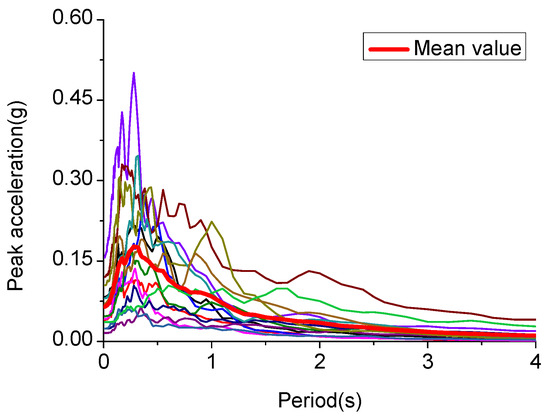
Figure 6.
Acceleration response spectrum for the fifteen ground motions.
The peak ground acceleration (PGA or A) of ground motions was chosen as the seismic intensity measure (IM), with a range of 0.05 g to 1.0 g and an incremental step of 0.05 g. Therefore, each ground motion was processed as having twenty amplitudes, yielding 300 ground motions after amplitude modulation. Then, 300 ground motions were randomly matched with the fifteen groups of the bridge analysis model. Each model group corresponded to twenty different ground motions, with PGA ranging from 0.05 g to 1.0 g; thus, a final total of 300 groups of bridge–ground motion analysis sample pairs were established.
3. One-Dimensional Seismic Fragility Analysis
3.1. Fundamental Theory of Seismic Fragility Analysis
Seismic fragility refers to the conditional probability of a structure or its components exceeding a certain performance limit state under different ground motions of varying intensities [35]; it can be generally expressed by the seismic fragility curves:
where is the seismic capacity of the structure or components and is the seismic demand of the structure or components. IM is a parameter used to evaluate the seismic intensity. Because in previous papers and are assumed to follow the normal distribution [35], Formula (7) can be simplified further as follows:
where is the standard normal distribution function and and are the logarithmic standard deviations of the structure’s or component’s seismic capacity and seismic demand, respectively. According to HAZUS99 [36], should adopt a value of 0.5 when PGA is used as IM.
3.2. Selection of the Damage Indexes
According to real seismic damage to actual bridges, the plate rubber bearing and the pier are most likely to be damaged under different ground motions. The plate rubber bearing is usually damaged because of the shear force, while the pier is usually damaged because of the bending moment. Therefore, the displacement and the displacement ductility ratio were chosen as the damage indexes for the plate rubber bearing and the pier, respectively [37]. The four seismic performance limit states of the entire bridge were defined to be slight damage, moderate damage, serious damage, and complete damage, respectively.
The moment–curvature analysis of the fifteen groups of the pier bottom section was performed by XTRACT to determine the threshold values of the pier under different performance limit states, and the corresponding ductility coefficients were obtained as well. Following the Seismic Retrofitting Manual for Highway Structures [38], the average seismic thresholds of the pier under four performance limit states were obtained based on the calculation formula related to the local displacement ductility capacity of the pier and the value of the pier column displacement ductility ratio, as shown in Table 5.
Table 5.
The seismic thresholds of the damage indexes under different performance limit states.
The allowable shear strain of the plate rubber bearing can be calculated using Formula (9). In accordance with the provisions of the Japanese Specifications for Seismic Design of Highway Bridges [39], this paper takes 100%, 150%, 200%, and 250% of the allowable shear strain as the threshold value of the plate rubber bearing under the four performance limit states. The corresponding displacement thresholds are calculated based on Formula (9), and are shown in Table 5:
where is the peak displacement of the plate rubber bearing and is the total thickness of the rubber layer.
3.3. The Seismic Fragility Curves of Single Components
The IDA method was first proposed by Bertero in 1977 [40], and is based on a sufficient number of dynamic time-history analyses that can reflect the seismic performance of structures under different ground motions of varying intensities in order to provide comprehensive and realistic evaluation of structural seismic performance [12,16,19]. This method has become widely employed in performance-based seismic engineering thanks to improvements in computational capability and structural analysis software. Therefore, the IDA method was employed to simulate 300 groups of bridge–ground motion analysis sample pairs based on OpenSees. The peak displacement of the plate rubber bearing and the peak displacement ductility ratio of the pier were calculated. The statistical information is shown in Table 6.
Table 6.
Statistical information for seismic demand.
The seismic demand of the structure or components is assumed to conform to logarithmic normal distribution [35], and the relationship between and IM should satisfy the following formula:
Taking the logarithm on both sides, we obtain
The fitting regression equations between and PGA are established by employing statistical regression analysis, as shown in Figure 7. The mean standard deviation of the fitting regression equations can be calculated according to Formula (12). A smaller indicates a better linear relationship, which is more suitable for the structural fragility evaluation index:
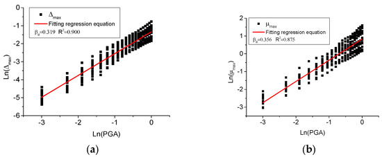
Figure 7.
Logarithmic regression analysis of single components: (a) plate rubber bearing and (b) pier.
When the fitting regression equations of the plate rubber bearing and pier are substituted into Formula (8), the following formulas for calculating the exceedance probability of single component under different performance limit states are further obtained:
The of the single components under different performance limit states can be determined according to Table 5. Employing the exceedance probability as the vertical coordinate and PGA as the horizontal coordinate, the seismic fragility curves of the single components under different performance limit states shown in Figure 8 are obtained.
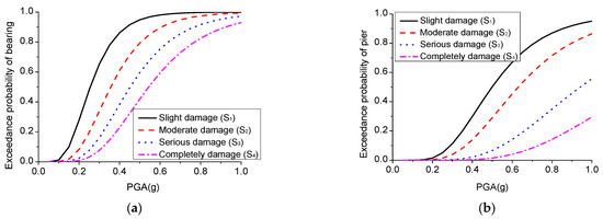
Figure 8.
The seismic fragility curves of single components under different performance limit states: (a) plate rubber bearing and (b) pier.
The exceedance probability of the single components under different performance limit states increases as PGA increases. Under ground motion with a PGA of 0.2 g, the exceedance probability of the plate rubber bearing and the pier in S1 stage is only 0.28 and 0.016, respectively, indicating that all components are in a good performance state. Under the ground motion with a PGA of 0.7 g, the exceedance probability of the plate rubber bearing in S2 stage is 0.80, indicating that the plate rubber bearing has been damaged to an extent and has potentially suffered serious damage. However, the exceedance probability of the pier in S2 stage is only 0.29, indicating that the pier has only sustained moderate damage. Under ground motion with a PGA of 0.9 g, the exceedance probability of the plate rubber bearing and the pier in the S4 stage is 0.89 and 0.21, indicating that the plate rubber bearing is almost completely damaged but that the pier would not collapse.
Comparing the seismic fragility curves of two components, the results show that the plate rubber bearing has a higher exceedance probability than the pier under different seismic performance states. The pier is the most important load-bearing component for the entire bridge, ensuring its overall seismic performance. The plate rubber bearing is the component connecting the pier and main beam, and has the advantages of simple, reliable, and convenient installation and replacement; thus, the ductility capacity of the bearing’s rubber layer is usually used for the energy consumption to reduce pier damage and avoid bridge collapse.
3.4. One-Dimensional Seismic Fragility Curves of the Entire Bridge
The seismic fragility curves of single components can directly illustrate the vulnerable positions of the entire bridge, providing an important reference for seismic performance evaluation and reinforcement of the entire bridge. However, bridge failure refers to the overall behavior, and the fragility of single components cannot represent the fragility of the entire bridge [12]. Based on the first-order reliability theory [41], relevant scholars assume that single components are either independent or completely correlated with each other, allowing the upper and lower bounds of the seismic fragility curve of the entire bridge to be obtained. Any single bridge component would interact with the others under actual conditions, and there is an internal correlation between the seismic response of single components. Therefore, the seismic fragility of the entire bridge should be within a range of upper and lower bounds, as shown in Formula (15):
The obtained upper and lower bounds of the seismic fragility curves of the entire bridge are shown in Figure 9. The results show that the lower bounds of the entire bridge coincide with the seismic fragility curves of the plate rubber bearing due to its vulnerable characteristics under ground motion. Although the first-order reliability theory has a simple concept and easily operability, it can only consider the correlation between seismic demand, not the correlations between the seismic capacity of all components. The seismic capacity of single components is determined by their structural seismic performance, which is characterized by the seismic responses of the single component. Thus, the seismic capacity of all components would have internal correlation due to the correlation between the seismic response of all components. Therefore, in this paper we investigated the seismic fragility of the entire bridge while considering the correlation between vulnerable components.
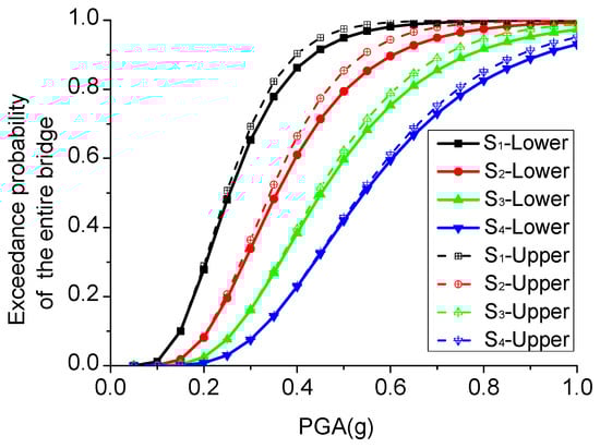
Figure 9.
Upper and lower bounds of seismic fragility curves of the entire bridge.
4. Two-Dimensional Seismic Fragility Analysis of the Entire Bridge Considering the Correlation between Vulnerable Components
4.1. Fundamental Theory of Multi-Dimensional Seismic Fragility Analysis
According to Cimellaro et al. [16], one-dimensional seismic fragility analysis can be extended to multi-dimensional analysis, and the formula of multi-dimensional seismic fragility curves of structural system can be further obtained, as shown below:
where is the seismic demand of each component and is the corresponding seismic capacity of each component under different performance limit states. Furthermore, the various performance limit states in the fragility analysis are related and random, allowing for the generalized formula of multi-dimensional performance limit state to be achieved.
where is the correlation coefficient of each component’s seismic demand, which can be obtained through experimental testing, seismic statistical data, or probabilistic seismic demand analysis. In this paper, the of the plate rubber bearing and of the pier are employed as damage indexes. Therefore, Formulas (16) and (17) can be simplified as follows:
where and are the two indexes of different performance limit states corresponding to the seismic capacity. For simplification, is assumed to be equal to and is assumed to be equal to 1; then, Formula (19) can be further simplified as follows:
where is used to measure the correlation between the plate rubber bearing and the pier under different performance limit states, which are the correlation coefficients of the vulnerable components.
4.2. Correlation Coefficients of Vulnerable Components
The diagram of the 2D joint performance limit state curves is shown in Figure 10. The elliptic curves represent the projection contour of the joint probability density function surface of the two evaluation indexes on the X-Y plane, and there are four performance limit state curves: Slight damage (S1), Moderate damage (S2), Serious damage (S3), and Complete damage (S4). When = 1, the seismic capability of two components is assumed to be completely correlated, and the performance limit state surface is projected as a straight line on the X-Y plane. When = ∞, the seismic capacity of two components is assumed to be mutually independent, and the performance limit state surface is projected as two vertical lines on the X-Y plane. According to the shape of the 2D joint performance limit state curves, directly affects the relationship between the performance limit state surface, and further influences the seismic fragility curves of the entire bridge. Therefore, the correlation between the seismic demand and the respective seismic capacities of the plate rubber bearing and the pier must be thoroughly investigated in order to obtain the fragility curves in accordance with the internal relationship of the structural seismic response.
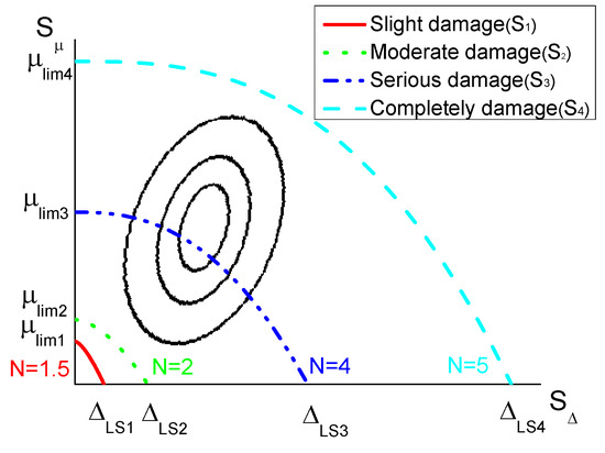
Figure 10.
Schematic diagram of the 2D joint performance limit state curves.
The Pearson correlation analysis method was used to calculate the correlation coefficients on the peak responses of the plate rubber bearing and the pier under different ground motions, as shown in Table 7. The relevant value can be obtained based on a fitting analysis. The results show that decreases as PGA increases. The bridge mainly performs the elastic response under ground motions with small PGA, and the between different components is massive. The entire bridge suffers nonlinear damage to a certain extent as PGA increases, and the between different components becomes smaller. According to Table 7, when the entire bridge is subjected to severe ground motions is approximately 0.8, indicating that the plate rubber bearing and the pier have significant relevance under severe ground motions. This is because the plate rubber bearing and the pier are connected directly, meaning that the seismic responses of the two components interact with each other. Due to the opposite correlation between and based on the correlation analysis, in this paper is taken as the reciprocal value of . Considering the short-changing of under various ground motions with different PGA, all values of under different performance limit states are chosen to be 1.215.
Table 7.
Statistical information for the correlation coefficients.
According to the seismic thresholds and between the plate rubber bearing and the pier under different performance limit states, the 2D joint performance limit state equations are as shown below:
4.3. Two-Dimensional Seismic Fragility Curves of the Entire Bridge
Following to Cimellaro et al. [16], the seismic response of the plate rubber bearing and the pier are assumed to follow the 2D joint lognormal distribution. The joint probability density of two components under ground motions with same PGA is as follows:
where , , and are the mean seismic response values of the plate rubber bearing and the pier, respectively, and are the logarithmic standard deviations of the seismic response of the plate rubber bearing and the pier, respectively, and is the correlation coefficient between and .
The correlation between the plate rubber bearing and the pier is thoroughly considered in this paper. The Monte Carlo algorithm was compiled by Matlab to obtain 106 samples with lognormal distributions. The random vector numbers falling into the structural failure domain were calculated in accordance with the equations under different performance limit states. Therefore, 2D seismic fragility curves for the entire bridge were obtained under ground motions with different PGA while considering the correlation between the plate rubber bearing and the pier. The 1D and 2D seismic fragility curves are shown in Figure 11.
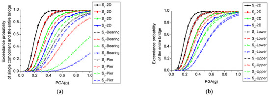
Figure 11.
Comparison of seismic fragility curves of the entire bridge: (a) seismic fragility curves of single components and the entire bridge; (b) 1D and 2D seismic fragility curves of the entire bridge.
Comparing the 1D and 2D seismic fragility curves, the 2D seismic fragility curve with consideration of the correlation between vulnerable components is significantly higher than the 1D seismic fragility curve of the entire bridge. Thus, considering only the seismic fragility of single components would overestimate the seismic performance of the bridge, which is consistent with the previous research [19]. In addition, the correlation between the vulnerable components cannot be ignored for the entire bridge due to their seismic interaction. Considering the correlation between vulnerable components, comprehensive and reliable seismic fragility curves can be obtained for the entire bridge. The PGA of S1, S2, S3, and S4 corresponding to 50% exceedance probability for 2D seismic fragility curves of the entire bridge are 0.19 g, 0.26 g, 0.34 g, and 0.40 g, respectively.
5. Seismic Risk Analysis of the Entire Bridge
5.1. Hazard Analysis at the Bridge Site
The most common site hazard analysis methods at present are empirical statistical methods, deterministic methods, and probabilistic methods. Because of the significant uncertainty in earthquake occurrence in terms of time, space, and intensity, the probabilistic method considers all potential seismic source areas for engineering sites as well as the possibility of ground motions at all levels in each potential seismic source area, and finally calculates the probability of ground motions exceeding a certain threshold at a given site, which is expressed in the form of a site hazard curve. As a result, it has become increasingly popular in recent years.
According to relevant research findings [42,43], spatial correlation exists between earthquake intensity measures. Considering the complexity of the effect mechanism, this paper adopts a point source model based on the concepts of exceedance probability and average return period in extreme value distribution theory [44]. Because the basic peak ground acceleration (A0) can be found in the Seismic Ground Motion Parameter Zonation Map of China (GB18306-2015) [45], with an exceedance probability of 10% during 50-year design reference period, A0 was employed to directly derive the calculation formula of the site hazard curve in this investigation. At present, scholars around the world generally acknowledge that the probability distribution of various seismic motion parameters follows approximately an extreme distribution [44,46,47]. Based on recent research findings [48], PGA is assumed to simulate the extreme value type II distribution with the following expression:
where is the PGA with the exceedance probability of 63.2%, is the shape factor, and the value in current seismic design codes is 6.87 when the seismic intensity at the bridge site is Degree 7 [49].
According to the relationship between the probability distribution function and the exceedance probability , Formula (26) can be further transformed as follows:
Taking the natural logarithms on both sides of Formula (27) and substituting the basic peak acceleration A0, the solution is solved simultaneously:
Because the current Seismic Ground Motion Zoning Map corresponds to the exceedance probability during a 50-year design reference period, the site hazard curve during a 100-year design reference period can be converted further. The calculation formula for the site hazard curve with PGA as the ground motion parameter can be obtained by substituting the conditions at the bridge site as follows: A0 = 0.20 g, = 6.87.
According to Formula (29), the exceedance probability under ground motions with different PGA is calculated, then the site hazard curve of the entire bridge is drawn using this as the ordinate and PGA as the abscissa, as shown in Figure 12.
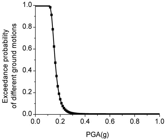
Figure 12.
The hazard curve at the bridge site.
In Figure 12, the exceedance probability of the ground motion decreases gradually as the PGA increases, indicating that the possibility of severe ground motion is decreasing. The site hazard curve drops sharply when PGA is between 0.10 g and 0.20 g, indicating that the probability of ground motion with PGA of 0.10 g to 0.20 g for the entire bridge is the highest. The site hazard curve can accurately reflect the design site’s hazard information, providing ground motion parameters for use in engineering seismic design.
5.2. Seismic Risk Analysis of the Entire Bridge
5.2.1. Mathematical Model for the Seismic Risk Analysis
The seismic risk analysis is a qualitative assessment at the probability level of ground motions of varying intensities and related social consequences that may occur in potential risk areas by fully utilizing site hazard analysis results and taking the fragility of disaster bearing bodies into account. It usually consists of three parts: seismic hazard analysis of engineering sites, fragility analysis of disaster bearing bodies, and seismic loss analysis. Seismic risk can be defined as follows: Seismic risk = Seismic hazard × Seismic loss = Seismic hazard for engineering site × Fragility of disaster bearing bodies × Seismic loss.
In this paper, the discrete conditional probability is used to represent fragility in order to simplify the calculation. The relationship described above can be expressed as follows:
where refers to the occurrence probability of the ground motions with PGA of that the structure may encounter during the design reference period, refers to the failure probability of the structure being in the j-class performance limit state when encountering ground motion with PGA of , and refers to the seismic loss risk when the structure is in the j-class performance limit state.
5.2.2. Calculation Process of Seismic Risk Analysis
The 2D seismic fragility curves and the hazard curve at the bridge site have already been obtained in Section 4 and Section 5.1, respectively. However, additional processing is required before beginning the seismic risk analysis due to the exceedance probability. According to the definition of seismic fragility, the structural failure probability of a specific level of performance limit states under ground motions of varying intensities can be calculated by employing Formula (31), as illustrated in Figure 13:
where refers to the structure’s basically intact state, refers to the exceedance probability that the structure may be in the j-class performance limit state when encountering ground motion with PGA of , and is the number of performance limit states, which is four in this paper.
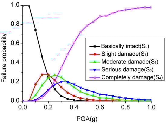
Figure 13.
Failure probabilities of the entire bridge under different performance limit states.
Similarly, according to the definition of the site hazard, the occurrence probability of ground motions of varying intensities during a 100-year design reference period can be approximately calculated by employing Formula (32), with the results shown in Table 8:
where refers to the occurrence probability of ground motions that the structure may encounter with PGA of during the design reference period and is the number PGA values, which is twenty in this paper.
Table 8.
Probability distribution of peak ground acceleration.
In view of the difficulty and subjectivity of estimating the indirect economic loss and direct input cost of earthquake relief, this paper only quantitatively estimates the direct economic loss of the entire bridge using the loss ratio defined by the American earthquake risk assessment system HAZUS [50]. The so-called loss ratio refers to the ratio between the maintenance or reconstruction cost and the initial cost of the structure under different performance limit states. Using the value indicated in Table 9, the loss ratio of the complete damage state is 2/, where is the total number of bridge spans.
Table 9.
The loss ratio under different performance limit states.
Now the seismic hazard and seismic risk probability for the entire bridge during 100-year design reference period can be calculated by employing Formula (18), as shown in Table 10.
Table 10.
The seismic risk probability for the entire bridge.
It can be seen from Table 10 that the seismic risk probability for the entire bridge ranges from 0.00454 to 0.00608. The bridge is most likely to remain basically intact or slightly damaged during ground motion. Although the loss ratio is relatively high when the structure is seriously damaged, the seismic hazard is less due to the small possibility of large ground motions. As a result, seismic disaster reduction research with respect to this bridge would focus on slight and moderate damage caused by moderate and small ground motions.
6. Conclusions
In this paper, the seismic risk analysis of an offshore bridge was investigated based on improved 2D seismic fragility analysis. The adverse effects of chloride ion erosion were considered, and a finite element analysis model of the entire bridge was established based on OpenSees. The seismic response process of the entire bridge was simulated employing the IDA method, and the displacement of the plate rubber bearing and the displacement ductility ratio of the pier were employed as damage indexes. The correlation coefficients of the plate rubber bearing and the pier under different ground motions were proposed based on Pearson correlation analysis, and the accurate 2D seismic fragility curves of the entire bridge were further obtained. The extreme value type II distribution theory was employed to directly derive the calculation formula of the site hazard curve, and the seismic risk probability of the entire bridge was finally achieved. The main conclusions are as follows:
- (1)
- Due to chloride ion erosion, the longitudinal reinforcement of the pier begins to corrode after 19.4 years, resulting in structural seismic performance degradation throughout the life cycle. The time-varying seismic fragility caused by chloride ion erosion must be comprehensively considered for offshore bridges.
- (2)
- When comparing the seismic fragility curves of two components, the results show that the plate rubber bearing has a higher exceedance probability than the pier under different seismic performance states. This is because the plate rubber bearing is often designed as a protective component in seismic design to ensure overall seismic safety performance. Due to the significant difference in mechanical properties between the plate rubber bearing and the pier, the upper and lower bounds of the 1D seismic fragility curves of the entire bridge based on first-order reliability theory are excessively broad.
- (3)
- Considering the seismic correlation between vulnerable components, the correlation coefficients were determined according to the Pearson correlation analysis method, then an improved 2D seismic fragility analysis was developed. The 2D seismic fragility curves for the entire bridge were comprehensively achieved, and are significantly higher than the 1D fragility curves based on first-order reliability theory. The results show that the seismic internal relationship between the plate rubber bearing and the pier cannot be ignored.
- (4)
- According to the 2D seismic fragility curves for the entire bridge, the PGA of S1, S2, S3, and S4 corresponding to 50% exceedance probability for the 2D seismic fragility curves of the entire bridge are 0.19, 0.26, 0.34, and 0.40, respectively, which can provide an important theoretical foundation and technical support for seismic design and performance evaluation of offshore bridges.
- (5)
- The site hazard curve drops sharply when PGA is between 0.10 g and 0.20 g, indicating that the probability of ground motions with PGA of 0.10 g to 0.20 g for the entire bridge is the highest. The seismic risk probability for the entire bridge ranges from 0.00454 to 0.00608. The bridge is most likely to remain basically intact or slightly damaged under different ground motions. Thus, seismic disaster reduction research for this scenario would be advised to focus on slight and moderate damage caused by moderate and small ground motions.
Author Contributions
Methodology, W.R.; Software, W.R.; Validation, W.R. and D.Q.; Formal analysis, D.Q.; Investigation, D.Q.; Writing—original draft, W.R. and D.Q.; Writing—review & editing, A.L. All authors have read and agreed to the published version of the manuscript.
Funding
This research was funded by [the National Natural Science Foundation of China] grant number [52208397], [the Natural Science Foundation of Shandong Province] grant number [ZR2021QE126] and [the Doctoral Research Fund Project of Shandong Jianzhu University] grant number [X20026Z0101].
Data Availability Statement
The data presented in this study are available on request from the corresponding author. The data are not publicly available due to fund requirements.
Conflicts of Interest
The authors declare no conflict of interest.
References
- Gu, Y.; Li, X.F. Seismic fragility analysis of offshore bridge structure considering chloride erosion. J. Basic Sci. Eng. 2019, 27, 1019–1032. (In Chinese) [Google Scholar]
- Zhong, J.; Mao, Y.H.; Yuan, X.Z. Lifetime seismic risk assessment of bridges with construction and aging considerations. Structures 2023, 47, 2259–2272. (In Chinese) [Google Scholar] [CrossRef]
- Li, H.N.; Cheng, H.; Wang, D.S. A review of advances in seismic fragility research on bridge structures. Eng. Mech. 2018, 35, 1–15. (In Chinese) [Google Scholar]
- Applied Technology Council (ATC). Next-Generation Performance-Based Seismic Design Guidelines-Program Plan for New and Existing Buildings; Federal Emergency Management Agency: Washington, DC, USA, 2006.
- Mackie, K.R.; Stojadinovic, B. Performance-based seismic bridge design for damage and loss limit states. Earthq. Eng. Struct. Dyn. 2007, 36, 1953–1971. [Google Scholar] [CrossRef]
- Padgett, J.E.; Desroches, R.; Nilsson, E. Regional seismic risk assessment of bridge network in Charleston, South Carolina. J. Earthq. Eng. 2010, 14, 918–933. [Google Scholar] [CrossRef]
- Kameshwar, S.; Padgett, J.E. Multi-hazard risk assessment of highway bridges subjected to earthquake and hurricane hazards. Eng. Struct. 2014, 78, 154–166. [Google Scholar] [CrossRef]
- Feng, Q.H.; Wang, W.C. Method and application of seismic risk probability analysis for large-long span bridge based on IDA-MC. J. Chang Univ. (Nat. Sci. Ed.) 2010, 30, 60–65. (In Chinese) [Google Scholar]
- Han, X.; Cui, S.A.; Cui, E.Q.; Su, J.; Zhu, B. Earthquake risk assessment of bridge based on failure probability method. J. Southwest Jiaotong Univ. 2018, 53, 696–703. (In Chinese) [Google Scholar]
- Xiang, B.S. Research on Time-Dependent Seismic Vulnerability and Risk Assessment of Prestressed Concrete Continuous Beam Bridges. Ph.D. Thesis, Southwest Jiaotong University, Chengdu, China, 2018. (In Chinese). [Google Scholar]
- Feng, L. Life Cycle Cost Analysis of High-Speed Railway Continuous Girder Bridge under Earthquake. Master’s Thesis, Lanzhou Jiaotong University, Lanzhou, China, 2020. (In Chinese). [Google Scholar]
- Wu, W.P.; Li, L.F. System seismic fragility analysis methods for bridge structures. J. Vib. Shock 2018, 37, 273–280. (In Chinese) [Google Scholar]
- Choi, E.; Desroches, R.; Nielson, B. Seismic fragility of typical bridges in moderate seismic zones. Eng. Struct. 2004, 26, 187–199. [Google Scholar] [CrossRef]
- Nielson, B.; Desroches, R. Seismic fragility methodology for highway bridges using a component level approach. Earthq. Eng. Struct. Dyn. 2007, 36, 823–839. [Google Scholar] [CrossRef]
- Song, S.; Qian, Y.J.; Wu, G. Seismic fragility analysis of a bridge system based on multivariate copula function. J. Vib. Shock 2017, 36, 122–129. (In Chinese) [Google Scholar]
- Cimellaro, G.P.; Reinhorn, A.M.; Bruneau, M.; Rutenberg, A. Multi-Dimensional Fragility of Structure Formulation and Evaluation; Report No. MCEER-06-0002; Multidisciplinary Center for Earthquake Engineering Research: New York, NY, USA, 2006. [Google Scholar]
- Wang, Q.A.; Wu, Z.Y.; Jia, Z.P. Multi-dimensional fragility analysis of bridge system. Eng. Mech. 2013, 30, 192–198. (In Chinese) [Google Scholar]
- Xiang, M.J.; Wang, X.J.; Wang, S.W.; Hu, B.; Li, C. BRB layout optimization and multi-dimensional fragility evaluation of multi-tower structure under stochastic excitation. China Civ. Eng. J. 2021, 54, 19–28. (In Chinese) [Google Scholar]
- Qiu, D.P.; Ren, W.J.; Chen, J.Y. The multi-dimensional fragility analysis of the underground large-scale frame structure based on the internal relationships of different seismic performance evaluating indexes. Tunn. Undergr. Space Technol. 2023, 136, 105093. [Google Scholar] [CrossRef]
- Caltrans. Seismic Design Criteria, Version 1.7; California Department of Transportation: Sacramento, CA, USA, 2013.
- Song, J.; Fan, Q.Q.; Feng, T.G.; Chen, Z.; Chen, J.; Gao, Y. A multi-block sliding approach to calculate the permanent seismic displacement of slopes. Eng. Geol. 2019, 255, 48–58. [Google Scholar] [CrossRef]
- Song, J.; Rodriguez-Marek, A.; Feng, T.G.; Ji, J. A generalized seismic sliding model of slopes with multiple slip surfacess. Earthq. Eng. Struct. Dyn. 2021, 50, 2595–2612. [Google Scholar] [CrossRef]
- Zhong, J.; Zhu, Y.T.; Han, Q. Impact of vertical ground motion on the statistical analysis of seismic demand for frictional isolated bridge in near-fault regions. Eng. Struct. 2023, 278, 115512. (In Chinese) [Google Scholar] [CrossRef]
- Liu, Y.; Weyers, R.E. Modeling the time-to-corrosion cracking in chloride contaminated reinforced concrete structures. ACI Mater. J. 1998, 95, 675–681. [Google Scholar]
- Cui, L. Mechanisms of Chloride Penetration into Concrete and Development of Profile in Marine Marine Environment. Master’s Thesis, Qingdao Technological University, Qingdao, China, 2010. (In Chinese). [Google Scholar]
- Li, C.; Li, H.N. Life-cycle Aseismic Performance Evaluation of Offshore Bridge Structures Considering Chloride Ions Corrosion Effect. J. Vib. Shock 2014, 33, 70–77. (In Chinese) [Google Scholar]
- Ghosh, J.; Padgett, J.E. Aging considerations in the development of time-dependent seismic fragility curves. Struct. Eng. 2010, 136, 1497–1511. [Google Scholar] [CrossRef]
- Ma, Y.F.; Zhang, J.R.; Wang, L.; Liu, Y. Probabilistic prediction with Bayesian updating for strength degradation of RC bridge beams. Struct. Saf. 2013, 44, 102–109. (In Chinese) [Google Scholar] [CrossRef]
- Zhang, W.P.; Song, X.B.; Gu, X.L.; Li, S. Tensile and fatigue behavior of corroded rebars. Constr. Build. Mater. 2012, 34, 409–417. (In Chinese) [Google Scholar] [CrossRef]
- Zhang, R.; Castel, A.; François, R. Concrete cover cracking with reinforcement corrosion of RC beam during chloride-induced corrosion process. Cem. Concr. Res. 2010, 40, 415–425. [Google Scholar] [CrossRef]
- Pan, Y.; Agrawal, A.K.; Ghosn, M. Seismic fragility of continuous steel highway bridges in New York State. J. Bridge Eng. 2007, 12, 689–699. [Google Scholar] [CrossRef]
- Wei, X.X.; Fu, B.; Wu, W.Y.; Liu, X. Effects of vertical ground motion on pedestrian-induced vibrations of footbridges: Numerical analysis and machine learning-based prediction. Buildings 2022, 12, 2138. [Google Scholar] [CrossRef]
- Zhang, N.; Pan, J.S.; Gao, Y.F.; Chen, X.; Dai, D.; Zhang, Y. Surface motion of an arbitrary number of semi-circular viscoelastic alluvial valleys for incident plane SH waves. Geophys. J. Int. 2022, 228, 1607–1620. [Google Scholar] [CrossRef]
- Dai, D.H.; Naggar, M.H.E.; Zhang, N.; Wang, Z. Rigorous solution for kinematic response of floating piles subjected to vertical P-wave. Appl. Math. Model. 2022, 106, 114–125. [Google Scholar] [CrossRef]
- Cornell, C.A.; Jalayer, F.; Hamburger, R.O.; Foutch, D.A. Probabilistic basis for 2000 SAC federal emergency management agency steel moment frame guidelines. J. Struct. Eng. 2002, 128, 526–533. [Google Scholar] [CrossRef]
- Federal Emergency Management Agency. Multi-Hazard Loss; Estimation Methodology Earthquake Model; Applied Technology Council: Washington, DC, USA, 2011. [Google Scholar]
- Hwang, H.; Liu, J.B.; Chiu, Y.H. Seismic Fragility Analysis of Highway Bridges; Mid-Ameirica Earthquake Center Technical Report, MAEC-RR-4 Project; The University of Memphis: Memphis, TN, USA, 2001; 38152, 2001. [Google Scholar]
- Buckle, I.; Friedland, I.; Mander, J.; Martin, R.; Nutt, M.P. Seismic Retrofitting Manual for Highway Structures: Part 1-Bridges; Federal Emergency Management Agency: Washington, DC, USA, 2006.
- Japanese Road Association. Specifications for Highway Bridges, Part V, Seismic Design; Japanese Road Association: Tokyo, Japan, 2002. [Google Scholar]
- Bertero, V.V. Strength and Deformation Capacities of Buildings under Extreme Environments. In Structural Engineering and Structural Mechanics; Prentice-Hall: Englewood Cliffs, NJ, USA, 1977; pp. 29–79. [Google Scholar]
- Zheng, K.F.; Chen, L.B.; Zhuang, W.L.; Ma, H.S.; Zhang, J.J. Bridge Vulnerability Analysis Based on Probabilistic Seismic Demand Models. Eng. Mech. 2013, 30, 165–171,187. (In Chinese) [Google Scholar]
- Garakaninezhad, A.; Bastami, M.; Soghrat, M.R. Spatial correlation for horizontal and vertical components of acceleration from northern Iran seismic events. J. Seismol. 2017, 21, 1505–1516. [Google Scholar] [CrossRef]
- Abbasnejadfard, M.; Bastami, M.; Fallah, A.; Garakaninezhad, A. Analyzing the effect of anisotropic spatial correlations of earthquake intensity measures on the result of seismic risk and resilience assessment of the portfolio of buildings. Bull. Earthq. Eng. 2021, 19, 5791–5817. [Google Scholar] [CrossRef]
- Cornell, C.A. Engineering Seismic Risk Analysis. Bull. Seismol. Soc. Am. 1968, 58, 1583–1606. [Google Scholar] [CrossRef]
- GB18306-2015; Seismic Ground Motion Parameters Zonation Map of China. Standardization Administration of China: Beijing, China, 2015.
- Algermissen, S.T.; Perkins, D.M. Probabilistic Estimate of Maximum Acceleration in Rock in the Contiguous United States; Open-File Report; USGS: Reston, VA, USA, 1982; Volume 82, pp. 76–416.
- Bastami, M.; Kowsari, M. Seismicity and seismic hazard assessment for greater Tehran region using Gumbel first asymptotic distribution. Struct. Eng. Mech. 2014, 49, 355–372. [Google Scholar] [CrossRef]
- Wan, H.P.; Wei, Z.C.; Su, L.; Ren, W. Seismic risk analysis of bridge structure considering pile diameter effect. J. Vib. Shock 2021, 40, 224–231. (In Chinese) [Google Scholar]
- GB50011 2010; Code for Seismic Design of Buildings. China Architecture & Building Press: Beijing, China, 2010.
- Department of Homeland Security, Federal Emergency Management Agency, Mitigation Division. MR4 Earthquake Model User Manual; Department of Homeland Security, Federal Emergency Management Agency, Mitigation Division: Whashington, DC, USA, 2009.


Disclaimer/Publisher’s Note: The statements, opinions and data contained in all publications are solely those of the individual author(s) and contributor(s) and not of MDPI and/or the editor(s). MDPI and/or the editor(s) disclaim responsibility for any injury to people or property resulting from any ideas, methods, instructions or products referred to in the content. |
© 2023 by the authors. Licensee MDPI, Basel, Switzerland. This article is an open access article distributed under the terms and conditions of the Creative Commons Attribution (CC BY) license (https://creativecommons.org/licenses/by/4.0/).