Article

Energy-Based Economic Sustainability Protocols

by
Federico Taranto
1,*,
Luigi Assom
2 and
Alessandro Chiolerio
3,*
1
Ecological Democracies—IT Department, Anthony Moddermanstraat 100, 1063 LT Amsterdam, The Netherlands
2
Nifty Works—Untangle Knowledge, Bellini 1, 31044 Treviso, Italy
3
Bioinspired Soft Robotics, Center for Converging Technologies, Istituto Italiano di Tecnologia, Via Morego 30, 16165 Genova, Italy
*
Authors to whom correspondence should be addressed.
Appl. Sci. 2023, 13(11), 6554; https://doi.org/10.3390/app13116554
Submission received: 7 March 2023 / Revised: 21 May 2023 / Accepted: 24 May 2023 / Published: 28 May 2023
(This article belongs to the Section Green Sustainable Science and Technology)

Abstract

:
In this paper, a sustainability framework for global and scalable payment systems is introduced. It is based on energy and resource consumption and pollutant classes and is inspired by ISO14040 principles. This paper aims to provide guidance for the implementation of blockchain-based technologies in a Life-Cycle Assessment methodology. The impact criteria adopted in this first approximation are at the stakeholders’ level. Enhancement through Enterprise Resource Planning software integration is considered to extend the impact allocation to the level of products and services. The system is designed on environmental economic models based on resources. A continuous depletion in the quality of exchangeable output is also modelled with respect to raw material consumption. We also consider the geophysical coordinates of pollutant emissions and the concurrent emission of pollutants affecting the quality of such outputs. This framework aims to be initially applied to the CO2eq indicator, which is identified by a set of aerial pollutants with global warming potential as proposed by the Intergovernmental Panel on Climate Change. Nonetheless, an incentive scheme within the so-defined payment system is possible and herein suggested, including the extension to other impact criteria (e.g., pollutants released in water and soil). Multiple approximations are made in order to overcome the difficulty in sampling reservoirs of natural resources, such as (1) disregarding regeneration rate and physical limits of raw material reservoirs and (2) estimating the minimum amount of pollutants affecting the perceived quality of economic transactions. Eventually, sampling policies are outlined as fundamental tactics to foster the effectiveness of this framework.

1. Introduction

The history of economics only started to account for sustainability issues at the beginning of last century. The physiocratic school was one of the early attempts to incorporate sustainability into economics by considering land as a primary resource for wealth generation [1]. Energy economics progressively emerged as a new approach that aimed to integrate sustainability accounting into economics. The energy economics approach differs from previous methodologies that dealt with externalities. Originally, it introduced the concept of energy cost as part of the production cost and provided a novel interpretation of value and its impact on society based on physical principles [2]: two examples are Pigou’s analytical solution, which aims to internalize external costs, and the Coasian approach, which sets an upperbound to social costs and allows transferring them in a secondary market [3,4]. In the last decades of the past century, environmental awareness further emphasized the need for sustainability accounting, and energy economics offered a way to recontextualize existing approaches: energy economics has the potential to posit a new basis of valuation that incorporates the principles of physics into economic relationships [5]. The goal of this paper is to emphasize the importance of transparent accounting systems with bottom-up decision-making processes and to propose a methodology that integrates Life-Cycle Assessment (LCA) into blockchain-based protocols for sustainable economies. The purpose of this work is to improve interoperability of LCA frameworks by contributing to overcome the limitation of utilizing proprietary data (e.g., Ecoinvent or SimaPro) [6], of lack of specificity of monetary data (e.g., Environmental Input–Output in Exiobase (EIO) (Environmental Input–Output in Exiobase—https://www.exiobase.eu/, accessed on 23 May 2023)), and of standardization of indicators and metrics [7,8].

2. Background

This work is motivated by the main limitations affecting: (i) the regulation of the commons, (ii) data accessibility and homogeneity in LCA accounting, and (iii) risks of misuse of environmental reporting (e.g., mismatches between the value of environmental resources that are physically bounded and their pricing).

2.1. Limitations on Impact Assessments

The concept of the commons refers to public resources that are freely accessible, but their regulation is often lobbied for business opportunities rather than preservation of ecological equilibrium (e.g., mitigating the discharge of a business’s external costs). In this paper, the term “commons” refers to energetic resources such as raw materials, air, water, and biological ecosystems, disregarding if property or usage rights exist in public or privatized form.
Life-Cycle Assessment (LCA) is a framework for assessing the potential environmental impacts of products; its adoption is challenged due to problems with consistency of data and consensus and exchange of life-cycle data. Examples of factors of data unavailability are legally binding (e.g., property or usage rights) non-homogeneous metrics and allocation methods and different standards in procurement activities [9]. Economic input/output models offer a less data-intensive approach than LCA methods [10] but lack specificity in accounting (e.g., allocating payment flows to specific commodity or company features [11]).
One challenge in embedding sustainability criteria in financial reporting for policymaking and risk assessment is the limited comprehensiveness of indicators in international frameworks. As an example, indicators solely relying on CO2eq may promote the adoption of technologies based on Rare Earth Elements (REE) without considering the effects of mining on common resources. Another concern is the lack of disclosure regarding the origin of procurement, which prevents open validation of actual allocations (e.g., utility companies claiming to produce renewable energy may use technologies that require non-renewable resources [12]); a deficiency of this kind is found in the Land Use, Land-Use Change, and Forestry (LULUCF) sector and in European regulations applied to the Emission Trading Scheme (ETS), which stated that biomass had an emission factor of 0 and its CO2 emissions could be withdrawn from total emissions (Part 5, section 2 in No. 601/2012/EU; point 15 in Decision No. 525/2013/EU and No. 529/2013/EU). This kind of uncertainty increases the risks of double expending and misuse of impact assessments in favour of stakeholders benefiting from competitive advantages in negotiation power or exercising exploitation rights. The economic nature of resources, characterized by different degrees of excludability and rivalry, exacerbates this problem. For example, air is considered fully non-excludable, while water is not always fully non-excludable. Additionally, water consumption and pollution are more sensitive to location due to its different physical state and control volume compared to air [13,14]. Therefore, water holds a higher degree of rivalry compared to air considering impact criteria of climate change [15].

2.2. Opportunities for Blockchain-Based Impact Assessment

Hybrid approaches embedding LCA and input/output models) in conjunction with blockchain-based payment tracking systems may improve the effectiveness and uptake of environmental assessment practices. Examples of potential applicability are traceability and accessibility of the historical transaction records of supply chains from origin to products and even by-products; persistence of and public access to data; and flexibility to elicit, design, and deploy consensus-based indicators that are universal for industrial domains and yet specific for each subdomain (e.g., metrics of global warming risks associated with by-product pollutants). Another benefit of blockchain-based payment-tracking systems is persistent data availability as an asset for computational sustainability research, such as in the field of reservoir computing [16].
On the whole, we consider that a strength of a blockchain-based protocol for impact assessment would be the capability to increase the resolution of environmental accounting measures and flexibly incorporate new metrics so as to address the need for more comprehensive indicators across industries [17]. We also argue that such indicators should be based on physically bounded resource availability (e.g., total available energy), so as to inform the economic activities that follow from use of resources, and from policies shaped on digital frameworks that could inter-operate through interconnected industries.

3. Materials and Methods

3.1. Circular Economy Reformulation: About Energy-Based Protocols on Resources and Impacts

In this section, we will critically discuss a reformulation of the circular economy concept that is particularly suitable for the sustainability framework described in this paper. While the circularity paradigm promotes the reuse of raw and recycled materials, resulting in a reduction in the depletion of raw materials, we encounter two limitations: (1) the circularity paradigm relies on information that incurs its own associated costs, and (2) it is bound by the second law of thermodynamics, which states that energy is inevitably lost in the form of waste heat during any energy conversion process. Thus, it should be complemented by other environmental frameworks. It is clear that there will always be consumption of materials and energy, which leads to the depletion of shared resources regardless of the degree of circularity within the economic paradigm.
Therefore, for our purposes, the impact of any economic system in terms of energy, raw materials, and emitted pollutants can be primarily quantified by evaluating its energy expenditure, which largely contributes to the depletion of shared resources in terms of both quality and quantity, as depicted in Figure 1. This remains true even when resources are completely recycled (in a fully circular economy). While it is not feasible to achieve complete resource recycling, it holds true to a certain extent, but the introduction of measuring common raw materials, tracking energy consumption, and evaluating their impact is becoming increasingly viable in today’s technological landscape. Notable advancements in energy trading systems and smart-metering hardware enable more-accurate LCA estimates in the food production sector [18]. This opportunity allows the allocation of users’ energy consumption to respective sets of pollutants derived from the impact assessment analysis of the energy source utilizing various approximation criteria [19,20].

3.2. Framework Boundaries

Required raw materials, energy exchanges, processes, and measurements are considered all along the life-cycle of products and services [21]. Due to lack of data, usually at the product and service level, it is common practice to refer to data of similar products or similar trade-offs. Nonetheless, an ad hoc analysis would be ideal, and an opportune incentive to foster its adoption is necessary for a truly sustainable society. Examples of best practices are certifications such as the Environmental Product Declaration (EPD), which defines Product Category Rules (PCRs) (a set of standards for sampling and analysis that needs to be performed for each specific product category in accordance with its composition or processing; also called single-company product-specific EPD, https://www.environdec.com/pcr-library, accessed on 23 May 2023)). In particular, categories of criteria concerning the EPD standards are provided in Table 1. Impacts, particularly from an LCA perspective, must refer to a gate-to-gate modelling approach, and therefore their allocation is only due to their respective stakeholder’s activity.

3.3. LCA Tree: Allocation, Aggregation, and Cut-Off

As previously introduced, each activity processes materials and energy to produce value in the form of finite products and services. Each activity, accounting for GHG protocol Scope 1, is responsible only for its direct contribution to the depletion of the environment. This means that at the Scope 1 level, a company that emits 3 Kg of CO2eq is only responsible for such an amount of CO2eq. Meanwhile, at the Scope 2 level, the amount of emissions generated by the considered activities is allocated to its energy production process. At the Scope 3 level, the amount of Scope 1 is incremented by the CO2eq emitted through all the prior activities supplied to the service of such company, including the supply of energy. This framework defines a multivariate approach, with features defined in Section 4.1.3 and Section 5.1 and better expanded in Appendix A.2 and Appendix A.4. This approach allows for a comprehensive and scalable scope definition, upgrading the current Scope 1, Scope 2, and Scope 3 categorization of the International Panel on Climate Change (IPCC) as well as other scopes as per those of the Global Reporting Initiative (GRI or EPD).

3.4. Impact Standardisation

Currently, LCA studies are conducted using various boundary conditions, such as gate-to-gate, cradle-to-gate, and cradle-to-grave, which refer to different stages of the supply chain. The absence of standardised metrics (e.g., EPD, ReCiPe, IPCC, and other protocols) and the inherent challenges in achieving single-score aggregation while maintaining the comprehensiveness of results are limiting factors for the development of robust models. In this paper, we limit our discussion to a single-score aggregation by using as an example the EPD standard with gate-to-gate boundary conditions. The values of each impact category should be standardised, either with the Z-Score (through statistical properties such as average and standard deviation) or m i n m a x normalisation (through the absolute maximum and minimum values in the whole dataset). Normalisation allows us to compare different patterns of signals whose magnitude may otherwise differ in size. Given that elicitation of weights and identification of the criteria are part of the decision-making and political process, for the sake of easier understanding, each weight will be set to 1 for each of the five criteria of the EPD certification.

4. Theory

In this section, the combination of the Energy Theory of Value is introduced to blockchain systems under an LCA perspective.

4.1. Energy Theory of Value

Starting from the commons introduced in Section 2, we will evaluate the surplus value that can be harnessed from raw resources and the externalities affecting their appreciation by any activity and, more broadly, by society. The idea is to shift the current economic evaluation to a valorisation that can create economic value for society more effectively [22]. To this purpose, we first associate the surplus value that can be extracted from common resources to the ability of society to generate productive means; then, we bridge these productive means to capital. This approach is inspired by physiocrats such as Quesnay and Turgot [23], who examined agricultural practices, and, more recently, by Serrano who examined non-agricultural productive activities [24]. With this approach, we contextualise the political economy aspects discussed in the formulation of the power theory of value by Nitzan and Bichler and lay the basis for an accounting of nominal (exchange value) vs. actual values (use value) [25]. We neglect the adoption of a financialisation based on capital as non-physical power (e.g., decisional dependence), as considered by Nitzan and Bichler, and rather focus on its physical features through implementation of the Energy Theory of Value to outline a new financialisation paradigm inspired by the previous work of several scientists in the last decades [26,27,28,29]. Particularly, we combine the trade value with the pleasure value, as defined by Stallinga [30], by grouping them in a subjective value form (e.g., use value) so as to extend the notion of mere physical quantities and overcome the limitation of net energy amounts as a policy planning tool—as pointed out by Hyman [31]. At the basis of this rationale, we consider that exergy represents a qualitative feature of energy transfer potential, as inspired by the previous work of Szargut in the indicator for cumulative accounting along supply chains [32] and Ayres for the bi-dimensional mapping of physical (energy/material) and subjective (value) dimensions [33].

4.1.1. Capital (Energy) and Debt

Considering physical commodities, we can harvest and transform existing reservoirs, which, in certain cases, are continuously renovated by external sources. The most important contribution to commons comes in electromagnetic form from the Sun. Natural storage of this constant flux may occur in multiple forms, mainly chemical (transformation of solar energy into cellulose by vegetable livestock and long-term creation of natural gas, coal, and oil reserves), thermal (heating of the atmosphere through its heat capacity, storage of charged energetic particles in the Van Allen belt, and heating of the oceans and landmass through their heat capacity), and kinetic (atmospheric circulation, thermo–haline circulation, water cycle, etc.). Another contribution comes from the radioactive decay of minerals that are thought to generate geothermal potential. Other common resources that can only be depleted are raw materials, such as technological metals and other elements such as rare earths, lithium, semiconductors, noble gases, and so on. Although accounting for the amount of energy stored in all raw materials retrievable on Earth could better help us understand the amount of surplus of wealth that can be potentially generated, let us disregard such a balance by justifying this choice with the fact that energy is needed in any case to extract and transform raw resources to make them suitable either for usage or for further energy extraction. The maximum ready-to-use energy availability (and therefore capital such as human labour, machinery, and commodities) that an economy can create while keeping its energy balance positive can be roughly approximated with the incoming solar net energy on Earth’s surface. Given the average value of 340 W/m2 estimated by NASA [34] and a surface of approximately 5.1 × 10 14 m2, the incoming power results to be approximately 1.7 PW; therefore, it is around 2 ZJ of energy per year ( 1 Z = 10 21 ). This amount could be trimmed to match the effective land surface of Earth, or fractions of it, but we feel that land-use allocation and technological capabilities remain a political decision, so we set the limit at a conceptual level at this stage. Although all this power may be potentially retrievable, technological and economic trade-offs imply a different reality. Nonetheless, this amount will be referred to as the maximum amount of energy that can be potentially used every year by a sustainable society. Therefore, as introduced in Section 5.2.2, the maximum amount of issuable debt that can be sustainably generated on Earth cannot be higher than the overall energy potentially consumed.

4.1.2. Use Value and Exchange Value

The statement that machines and humans produce a different quality of work is colliding nowadays with the increase in flexibility and efficiency of Artificial Intelligence (AI)-powered systems. The usage of statistical and logical methods for simulating complex decision-making capabilities has nearly approached the level of creativity that humans possess.
Energy is, regardless, always required. Considering that labour is a transformed form of energy, humans as biological thermodynamic machines, and a colliding relation between exchange value and use value [35], let us take the use value for the accounting of externalities affecting the utility of purchasers [36]. In this analysis, behavioural science will not be discussed in detail; therefore, let us consider this function as a random variable for now. Let us also justify this approximation by stating that information retrievable—for a high number of stakeholders—allows us to consider it only as white noise with known statistical properties. Part of the scope of this paper is to allow the gathering of the metrics for a heuristic assessment of the distribution of such statistical properties at an operational stage. Furthermore, let us define the resultant benefit that drives the feasibility of a transaction for the buyer as the maximum between the exchange value of the activity (exv) and its subjective value (usev) for the buyer:
b e n e f i t = max ( u s e v , e x v ) = max ( f ( U i , j ) , O i , j )
where f(Ui,j) is a function of the personal needs of the stakeholders towards the activity (or a set of activities) i purchased from stakeholder j. Oi,j is the exchange value of the activity, and Ui,j is the utility of the buyer towards the output generated by the activity of the considered seller.

4.1.3. Measuring the Exchange Value

Based on the work of Szargut and Morris [37], we use the CExC to be able to account for raw materials and energy and for the perfection of production processes leading to the activity (or supply chain) under consideration. The value of the activity can be expressed as the energy consumed ( E i , j ) plus the value of the materials processed by the stakeholder to create a certain output of its activity ( C H ( N ) ), where H represents the set of extracted flows from the common reservoirs for a degree of depth of the analysis N.
O i , j = C i , j H ( N ) + E i , j
The wealth O i , j in this case represents the exchange value of the produced output, which is an objective and quantitative reference of value. However, in addition to this value, we need to consider the subjective difference in cost or benefit, as defined in Equation (7), which relates to the value of the common as defined in Equation (1). The customers’ willingness to pay will also depend on the environmental externalities generated by each activity, which, in our first approximation, are captured through a custom utility function that is dependent on socio–economic aspects. The internalization of these social costs will be discretised in a time unit and referred to as the Stakeholder’s Responsibility Paradigm (see Section 5.1), considering that stakeholders as well as industrial policymakers fully internalize them as a cost upstream from their supply chains. For now, let us continue deriving the dependence of activities on each other and on the raw materials and resources stakeholders process and extract. Using Equation (2) and knowing that the value of the commodities in input CH(N) is the weighted composition of the value of commodities purchased by the supplier plus the energy consumed to process them and proceeding recursively until extraction from the reservoir of the considered resource (e.g., N = ), we can define the energetic cost as:
E i , j = μ i , j ϕ i , j ψ i , j C i , j
where:
μ i , j = efficiency [ % ] ϕ i , j = compound exergy [ k W h K g C i , j ] ψ i , j = energy price [ EUR k W h ]
The term KgCi,j in Equation (4) is the weight of the resource used by j to produce activity i. Equation (2) can be rewritten as the summation over all users belonging to the tree of the transaction (p) considered; we drop the index j for simplicity:
O i = p π ( N = ) μ p ϕ p ψ p R p
where:
R p = R p * [ k g m 2 · y r ] · A p [ m 2 ] · Δ t i [ y r ]
The term C i , j in (4) is now substituted by the term R p , which represents the intake from common resources R as specified in (7). Equation (5) represents the relation between the exchange value of an activity to all the activities it depends on and the raw resources dispersed over an area A, whose depletion occurs during a time Δ t . The term π stands for the whole set of transactions limited by a degree of depth, or accuracy, N; while p stands for the current level of the transaction tree being accounted for. Both sizes will be further described in Section 5.1. The density of the extraction capabilities of the raw materials over a considered area is defined via Equation (6), where the surface and time units have been expressed in m 2 and y r , respectively. It is worth pointing out that this cumulative expression of energy exchanges, represented in the form of embodied wealth, is already integrated along time units through the term Δ t . This formulation will be re-contextualised in (11).

4.2. Evaluation of Societal Wealth

This paragraph introduces the theory for evaluating societal activities, which mirrors the quantifiable energy metrics previously introduced and contributes to defining the objective wealth of an economy.

4.2.1. Quality of the Common

The quality of activity output (and of the resources) is an important concept in the proposed theory. It does not only identify a part of the utility any user can perceive from a certain activity, as defined in Equation (2), but also its physical properties that affect the utility of its usage and, therefore, the subjective value component of any stakeholder. The “quality” of a stream of by-products (waste matter/energy released into the environment by any activity, waste heat being the biggest energy flow mankind is generating, as big as 142 PWh/y [38]) represents the availability of harnessed energy therein contained. In the context of stakeholders or species interacting with toxic, carcinogenic, or mutagenic compounds dispersed into matter or energy flows, the concept of exergy in thermodynamics can be used to represent the potential energy contained in such streams of by-products [39]. This qualitative feature of matter and energy, which represents also the potential to retrieve energy from materials or to cause harm to the same stakeholder, is mapped according to the availability of users to pay for the activity that creates said feature. As exergy represents the entire potential of energy state changes in relation to an environment that normally provides lower grade enthalpy for exchanges, so stakeholders’ utility functions represent wealth changes of the seller due to the utility of their products to the buyer (both for products, waste, and irreversible waste that cannot be recovered, such as dispersed emissions) in relation to both system states.
Let us refer to this resulting economic outcome of the quality of output as commons depletion/restoration due to the modification of the intrinsic value of the resources or, economically speaking, to the externalities that the considered activity creates in the appreciation of such value.

4.2.2. The Value of the Common

What would be the value of a resource without any living creature being able to use it? In the specific case of Intellectual Property (IP) issues, the resources required for knowledge production are a form of energy, such as food, electricity, information, and experiences, that bring inventors and innovators to a certain result. It is energy that generates information. IP value is not only the energy required to produce it nor its agreed material value; rather, it is a subjective expression of the buyer. Therefore, without stakeholders producing added value through exchanges (activities) and depleting the resources, there would not be any initialization of such a concept to account for. As such, in this model, all resources will be ordered according to stakeholders’ use: in other words, purchase transactions rather than in a physical spatio–temporal locus. Let us call C the value of the common, and R is the value of all raw materials extracted for the production of the activities of stakeholders j belonging to ensemble J, all of them involved in transaction i, which is part of the total set of transactions I. Let us continue to add to the resources used for common economic purpose the difference between the subjective value perceived by the purchaser and the (energetic) production cost of the considered transactional value exchanged by the seller. The dynamics defining this term will be represented by the demand and production cost curve of the stakeholders involved in the transaction through the relation expressed in Equation (1). The value of the common will be the value of all raw materials possessed (resources extracted) by these stakeholders plus the subjective value of all stakeholders generated by the exchanges of such goods:
C = R + i , j I , J Π max ( u s e v i , j e x v i , j [ P i , j ] , 0 ) u s e v i , b u y e r = f ( U i j , b u y e r ) see Equation ( 1 ) e x v i , s e l l e r = O i s e l l e r see Equation ( 2 )
The term Π stands for the transaction tree of the whole system and embraces the set of all transaction trees π , as defined in (5). Pi,j represents the impact cost created by the seller j of the considered transaction i. This term is surrounded by square brackets to indicate that it can be considered only if the cost relative to the impacts under analysis can be quantified. In case the cost of such impacts cannot be quantified (e.g., due to the complexity of modelling pollution, the complexity of toxicology dynamics, etc.), the term P i , j is accounted as affecting the utility function of the term u s e v i , j . This is equivalent to considering information on pollutants affecting purchases while disregarding the spatio–temporal locus, considering, therefore, that pollutant emission influences stakeholders and their transactions ubiquitously and instantaneously. The removal of noxious emissions is considered a negative social cost, while its injection into the environment is a positive social cost. This choice is due to the harmful effects on living beings of noxious compounds [40]. The hypothesis behind this assumption is that externalities occur because production is satisfied by the demand (that creates the transaction), whose value represents the value subjectively perceived by the buyer. No assumptions are made about the properties of the commons: the framework we use must be seen from a holistic point of view—that of the ecosystem.

4.2.3. Evaluating the Costs of Impacts

The utilitarian internalisation can be considered, as defined in Section 4.2.2 (omitting the impact term and considering the ubiquitous and immediate knowledge of stakeholders), in case it is not possible to describe how pollutants can affect the economies of society, either due to the lack of markets for a specific pollutant or due to the lack of modelling and sampling schemes. Let us introduce the theory for evaluating tradeable pollutants whose impacts and costs can be quantified. We define the monetized impact Pi,j, referring to an activity i operated by the stakeholder j, as:
P i , j = p i , j τ C i , j
where:
τ = EUR S . I . U . = impact value p i , j = S . I . U . k g i , j = impact unitary rate
and:
C i , j = C i , j * [ k g m 2 · y r ] · A i , j [ m 2 ] · Δ t i [ y r ]
The relationship between quantity and externalities is assumed to be linear. It can be also described by higher-order functions, though this implies higher computational costs for the identification of sustainable policies. In case this framework is applied only to CO2eq, τ refers to the carbon market price. In case of multiple impacts instead, the weighting of the criteria will be calculated according to the standardisation defined in Section 3.4. In case of a positive impact to or mitigation of resource extraction, the regenerative rate or depletion rate can be accounted for as an impact once the values and the amounts of the resource regenerated or depleted are known. The figures introduced in the previous equations are listed in Table 2.

4.3. Time-Discrete Activities, Overcoming a Lack of Raw-Material Tokenization

For example, let us consider Bob buying a product from Alice. By knowing only the impact of Alice’s operation and assuming Alice will provide different products/services as the output, we cannot allocate the impact of inputs (resources such as energy, input commodities, and raw materials) and processing labour for only the product purchased by Bob. Therefore, this sustainability protocol must be integrated with ERP (Enterprise Resource Planning software) data in order to operate at the product/service level, otherwise the economic canvas can be redistributed only at the stakeholder level. Nonetheless, we can consider impact and resource responsibilities related to the overall set of products/services produced in a time unit t t 0 = Δ t s y s , defined as the time-step for the economic protocol, by a stakeholder j, and considering energy expenditures of the same stakeholder in the same time unit, expressed by the following relation:
E j = t 0 t E i , j Δ t s y s P j = t 0 t P i , j Δ t s y s C j H ( N ) = t 0 t p π ( N , j ) C p H Δ t s y s
By doing so, we will be able to discretize differences among stakeholders’ transactions and processing intervals and the pace of the system’s accounting for transactions. For the sake of clarity, we dropped the subscript j in Equation (11), which represents the stakeholders whose activities belong to the transaction tree of stakeholder j.

5. Results

In this section, the conceptual results obtained by application of the protocol defined above are shown. For clarity, we recall that the definition of the protocol is the combination of Equations (2), (3), (5)–(8), and (10) and the boundary conditions defined in Figure 1. The result is a system represented in Figure 2, where cylindrical shapes are entities of the protocol and trapezoidal shapes are processes that upgrade the entities of the protocol. The Social Cost Compensation in Figure 1 is now called Compensation and is provided thanks to stakeholders that spend energy to compensate for the cost of energy consumption of other stakeholders in an energetic, material, or informational form. Further implications of the results discussed hereafter can be found in the Appendix A, Appendix B and Appendix C.
The synchronisation process among nodes is therefore a transparent standardisation process of LCA locally validated data. We are now going to discuss more detailed implications.

5.1. A Tool for Industrial Policies: Stakeholder’s Responsibility Paradigm

Considering a policymaker whose intention is to evaluate the industrial strategy that creates more wealth for a certain set of stakeholders at a certain level of the supply chain, from a given stakeholder, proceeding upwards until level N in the procurement of energy and input materials required for the activity of any stakeholder over the time unit t t 0 , the wealth balance of a j th stakeholder can be defined by the following equation:
O j = C j H ( N ) R e s o u r c e s + E j p ( j ) π ( N , j ) P j j , j + 1 N th s c o p e
which derives from Equation (2) and the social cost defined in Equation (7). The cost of externalities is hidden by the producer, therefore resulting in a decreased value of the produced wealth. The O stands for Output and is represented by a monetary size, while C represents the commodities in the input, as a sum of the withdrawn value of all raw materials H for the considered degree of accuracy of the impact assessment N. P is the impact generated, represented as wealth depletion. The sum on the right-hand side refers to the transaction level of stakeholders. Particularly, superscript j, j + 1 refers to the stakeholder at level j to the stakeholder at level j + 1 , where j purchases from j + 1 . N represents the degree of accuracy of the impact allocation threshold, further explained in Appendix A.2, while π is a subset of Π introduced in (7). Particularly, j is the counter for the depth-level of the analysis (at the transaction/procurement level); this refers to the considered stakeholder whose impact is being cumulated. The grouped references Resourcesand Nth scope in Equation (12) represent, respectively, the Resource and the Nth-scope component of this model. Introducing the definition of the wealth from raw materials (R) from Equation (5) and substituting it into Equation (12), we can write:
O j = p ( j ) π ( N = , j ) μ p ϕ p ψ p R p p ( j ) π ( N , j ) P j j , j + 1
Stating that the value of the overall activities produced by stakeholder j in the time span t t 0 is equal to the algebraic sum of the energy produced for the extraction of all the required resources, both for electricity production (e.g., energy carriers such as coal or uranium) and raw materials (e.g., water and minerals) consumed in the interval t t 0 minus the sum of the impact the stakeholder is responsible for, which affects its supply chain upstream. Please note also that the energy produced is proportional to the value of the energy exploitable from the compound and to the price at which such energy can be sold to the market, as well as to the efficiency of the transformation. For raw material extraction, it is the maximum of the energy retrievable from raw materials (an example can be found in [41]) and the minimum amount of work required to extract such resources [42]. In this context, the coefficients μ , ψ , ϕ can be considered as weighted averages of the respective sizes of all process-specific activities generated by stakeholder j in the time unit t t 0 .

5.2. Grouped Interests

In this section, the theory for the accounting of grouped stakeholders pursuing a joint strategy is discussed. The group of stakeholders can be any conglomerate of decision-making votes. It can be represented by countries, local communities, or even by blockchain nodes. Each member of any of these groups is thought to contribute to the political vote of the group according to the criterion defined by the group (e.g., the land each user’s activity insists on, the energy consumed, etc.; see Section 5.4).

5.2.1. Wealth of Territories

By territories, we mean not only countries, but also any land extension where labour exists as a part of an economy that processes resources through a network of value exchanges based on interests. From aggregation of the user value for all users J within a certain territory z, the wealth balance of the territory can be written as follows:
O z = j J ( z ) O j = C z H ( N ) + j J ( z ) E j + j J ( z ) P j
where C z stands for all commodities produced in the territory z from the needed set of raw materials H and for a cutoff N of the protocol. The summations E j and P j stand for all energy expenditures and respective social costs generated by the stakeholder j. Please note that in the above equation, the N th scope term is not present, compared to the stakeholder’s responsibility paradigm (see Section 5.1). Given its subjectivity, in terms of stakeholder’s perceived value, is not necessarily reflected in an objective impact on society, therefore the term f(U), as defined in Equation (1), is omitted. We note the fact that the countries distribution is not necessarily based on a territory map: federations of countries where goods (or services, or information) are produced and transported can still offer a sustainable solution, thus keeping well-balanced wealth and accommodating for local unbalances globally.

5.2.2. Land Use Issuance Cap

As introduced in Section 4.1.1, irradiance being equal to γ and considering ideal efficiency to transform energy into work, the maximum amount of debt we can issue per country z can be given by the following equation:
I ( O t ) = max ( O t z , A , t γ ψ A A t o t d t d A )
where ψ is the price of electric energy, and O t z is the total value produced by all activities of the stakeholders in the country z during the time interval t. The irradiance value, γ , is dependent on time, latitude, and longitude of the country from a first-order approximation and is, therefore, integrated along the time and the surface of the country. The term A / A t o t is a redistribution coefficient to account for differences in area extension of lands of different communities, with A t o t being the total surface of the globe. Different criteria could also be defined, for example, by including other external indicators or weighting the irradiance with a redistributive coefficient.

5.3. Sustainable Minting Function: Keen Universal Basic Energy

The green arrows in Figure 3 represent the energy purchased or sold by different stakeholders and, therefore, the credit (+) or debit (−) they get rewarded with for the potential they have in creating value to society from such energy exchanges. Let us name this concept Keen Universal Basic Energy (KUBE) in honour of the person who first introduced this term. Through this instrument, users are provided with an amount of currency unit proportional to the energy consumed and to the inverse of its impact (more complex indicators can be defined for the KUBE function).
i = | E i , j | P i , j if P > 0 i = P i , j | E i , j | if P 0
It is worth noting that each of the represented stakeholders can take the role of an energy banking supplier. This framework is intended to facilitate the sustainable adoption and extension of carbon credit schemes and other impact assessment criteria to activities that not only produce energy, as is currently the case, but also any other product or service. Considering this system as a payment network, accounts are expected to have a unique identifier or address, which might be related to sensitive information required by local jurisdictions. The anonymity of stakeholders is of paramount importance in the adoption and acceptance of any payment system: privacy concerns can be addressed by clear rules embedded into an appropriate minting function, which can also allow analysis of economic flows for scientific research purposes.

5.4. Node Consensus for Pollution Sampling Schemes

Impact aggregation to a single score is necessary to compare and rank activities for distributing financial incentives. This process is very sensitive to the weight of parameters used for the aggregation. In this paper, integer values for all indicators are considered as defined above by the EPD standard. Nonetheless, particular aggregation rules can be specified after geographical, social, and environmental economic analysis for the attainment of specific targeted needs of reduction or increase for any criterion (e.g., see Section 3.4). This process can be implemented through different nodes that interact with each other automatically to manage the conversion of different weights and criteria adopted in a transparent manner.

5.5. The Role of a Payment Tracking System in the Depletion of the Commons

Let us consider two companies that own land located above a natural water spring (having neither a well nor smart metering hardware), and let us suppose that the local legislation allows these companies to be entitled to exert full control over the raw materials located on their property. Now let us suppose both companies decide to bottle natural water, collecting it from two natural springs, and both are harvesting it from the same groundwater reservoir. Satellite imagery may provide an effective tool for assessing water withdrawals for better planning of water reservoirs [43]. However, discriminating stakeholders’ individual consumption for nearby withdrawals from the same reservoir may be challenging. Therefore, tracing the amount of water harvested from the environment by focusing on monitoring the event of water depletion while maintaining spatio–temporal resolution is not as effective as focusing on anonymous stakeholders’ behaviour in known locations would be.

5.6. About Extractors, Recyclers, and Optimizers

Any activity that mitigates resources consumption can be given a special role. The laws defining the energetic costs and the impact of the regeneration activity for any resource are defined the same for the energy providers, particularly as per Equation (3). Considering a set of stakeholders inside an approximated supply chain, as shown in the diagram of Figure 3, the extractors are set in red and the blue arrows stand for the wealth generated due to resource restoration. We might consider particular activities that are conceived to optimize or reduce expenses under special circumstances while processing and consuming energy. For example, climate change has statistically increased the likelihood of dealing with floods, droughts, and storms. Investing money and energy to spatially reconfigure raw materials is a way to optimize resources without necessarily depleting them in order to reduce the risk of disasters, which would imply much higher reconstruction costs. Scientific research and the IP it produces also belong to an optimization problem characterized by unknown spatio–temporal scopes: constant investments will generate, randomly, optimization of resources, new stakeholders, new resources to be depleted, and new energy channels to utilize.

6. Conclusions

In conclusion, we have shown a possible way of tackling sustainability challenges nowadays. These being a widespread adoption of sampling of externalities and the integration of impact assessment into economics, we have proposed a methodology for integrating such two aspects, overcoming the concerns of confidentiality of supplier information with anonymous stakeholder reward systems. Particularly, the adoption of public blockchain databases enables transparency of scientific research over a persistent data layer and promotes progress in standardisation through heterogeneity of interconnected domains. Bottom-up ingestion and withdrawal of credit from energy consumption (data retrieved from electricity consumption metering devices) were discussed as approaches to avoid wealth-distribution issues. An initial model framing resource-based economics was proposed in the context of the blockchain protocol, where model constraints are defined as energy retrievable per land-use allocation. A set of general criteria for impact assessment of resource depletion and pollutants was proposed as a component to facilitate, in their simplicity, global scalability and adoption and to create intrinsically sustainable economies whose sustainability impact is digitized at the transaction time and persists in a globally accessible protocol. Finally, we have discussed the political need to incentivize sampling and standardisation of impacts among all stakeholders in a supply chain as a condition towards comprehensiveness and adoption of sustainability frameworks.   

Author Contributions

F.T.: Conceptualization, Methodology, Investigation, and Writing—Original Draft. L.A.: Critical revise, Writing—Review and Editing. A.C.: Supervision and Writing—Review and Editing. All authors have read and agreed to the published version of the manuscript.

Funding

This research received no external funding.

Data Availability Statement

No new data were created or analyzed in this study. Data sharing is not applicable to this article.

Acknowledgments

The authors would like to thank Matteo Rocco for his feedback, Marco Guido Ponti and Steve Keen for providing constructive insight and critiques, and F.J. Duijnhouwer for clarity of national practices of impact allocation and frameworks.

Conflicts of Interest

The authors declare no conflict of interest. This research did not receive any grants nor directives from funding agencies in the public, commercial, or not-for-profit sectors.

Nomenclature and Abbreviations

The following nomenclature and abbreviations have been used in this manuscript:
CExCCumulative Exergy Consumption is an indicator introduced by Szargut [32] in 1987. It integrates exergy accounting as an ecological and thermodynamic indicator for the assessment of production processes and supply chains.
CFCommunity (-based) Forestry is the concept of local communities that, when granted sufficient property rights over local forest commons, can organize autonomously [44].
cradle-to-gateCradle-to-gate is a boundary condition of LCA analysis. It refers to an assessment of the life cycle of events related to the production of a good from the extraction of raw materials required for its fabrication until the product’s sale [45].
cradle-to-graveCradle-to-grave is a boundary condition of LCA analysis. It refers to an assessment of the life cycle of a product from the extraction of raw materials required for its fabrication, until its use and disposal.
EIBEuropean Investment Bank. The EIB has as shareholders the EU member states.
EPDEnvironmental Product Declaration is a report standard that states what a product is made of and how it impacts the environment across its entire life cycle. It is defined by International Organization for Standardization (ISO 14025) as a Type III declaration [46]. It enables comparisons between products fulfilling the same function. For more information, see: www.environdec.com, accessed on 23 May 2023).
ETSEmission Trading System is a market mechanism that limits by a ’cap’ the number of emission allowances. In this paper, ETS is particularly referred to as European emission trading system (EU ETS). https://ec.europa.eu/clima/policies/ets/cap_en, accessed on 23 May 2023.
exchange valueThe objective value given as the cost of production sustained by the seller to create a particular activity [47].
externalitiesExternal costs that are not computed in the production cost by the producer given the divergent interest among the decisional criteria of the producer (e.g., minimization of cost) and the internalisation of its social cost [48].
FDIForeign Direct Investment is an investment made by a firm or individual resident in one specific country into business interests located abroad.
gate-to-gateGate-to-gate is a boundary condition of LCA analysis. In this paper, gate-to-gate refers to the boundary condition from the procurement of the resources until sales of goods. Therefore, it is only referenced in the production stage of the considered activity.
GHGGreenhouse Gases are those gaseous constituents of the atmosphere, both natural and anthropogenic, that absorb and emit radiation at specific wavelengths within the spectrum of thermal infrared radiation emitted by the Earth’s surface, the atmosphere itself, and by clouds. This property causes the greenhouse effect.
GRIGlobal Reporting Initiative is an international standards organization that helps businesses, governments, and other organizations to understand and communicate their impacts. https://www.globalreporting.org/, accessed on 23 May 2023.
IMFInternational Monetary Fund. https://www.imf.org/en/About, accessed on 23 May 2023.
IPIntellectual property refers broadly to the intangible creations of the human intellect.
IPCCIntergovernmental Panel on Climate Change is a paragovernmental organization based in Switzerland. Website: www.ipcc.ch, accessed on 23 May 2023.
irradianceIrradiance is the net amount of electromagnetic energy per unit of area that hits the Earth’s surface. It depends on the spectrum of the incoming source, on the absorbance characteristics of the atmosphere, and on the incident angle with respect to the planet surface.
ISOThe International Organization for Standardisation is an organization that brings together experts to share knowledge and develop voluntary, consensus-based, market-relevant International Standards. https://www.iso.org/home.html, accessed on 23 May 2023.
LCALife-Cycle Assessment methodology, the conjunction of impact assessment to life-cycle inventory analysis.
ReCiPeReCiPe is a method of Life-Cycle Impact Assessment (LCIA). It was first developed in 2008 through cooperation between Rijksinstituut voor Volksgezondheid en Milieu, Radboud University Nijmegen, Leiden University, and PRé Sustainability
REDD+Reducing Emissions from Deforestation and forest Degradation is a monetary incentive framework idealised by United Nations in Midtown Manhattan, New York City, United States. and having its claimed purpose as the conservation and sustainable management of forests and enhancement of forest carbon stocks in developing countries.
resourcesA resource is a source or supply from which a benefit is produced and that has some utility. Throughout this paper, the term resource is used to identify both the raw material (e.g., air, water, minerals, etc.) and output of production activities, if not otherwise specified.
Scope 1Scope 1 emissions are direct emissions from sources that are either owned or controlled by stakeholders.
Scope 2Scope 2 emissions are indirectly produced by the generation of purchased energy.
Scope 3Scope 3 emissions are all indirect emissions (not included in Scope 2) that occur in the value chain of the reporting company, including both upstream and downstream emissions.
Type III declarationEnvironmental label or declaration that provides quantitative environmental data using predetermined parameters (based on the ISO 14040 series of standards) and, where relevant, additional environmental information in the form of quantitative or qualitative information.
use valueThe subjective value, or usefulness, that a transaction has for the buyer [47]. Such value is defined only if higher than the exchange value of a transaction or higher than the value of the transaction plus the social cost (if not previously internalised at the production stage by the seller).
user groupsGroups of stakeholders in charge of managing CF practices. These groups are committees having the same interest with respect to the CF policies defined by the governmental authority that provides the ownership of the land.

Appendix A. Featuring the LCA Framework

In this section, different guidelines for the creation of the LCA framework are introduced; these are the same as the guidelines followed in creating this protocol.

Appendix A.1. Lack of Sampling Penalty

In case stakeholders do not declare their impact, its sampling and communication can be incentivized by considering the maximum impact registered by the system for similar activities. Similar incentive mechanisms can be adopted to foster the sampling of activities whose impact is assessed to be far bigger than the average activity of the system.

Appendix A.2. LCA Boundaries and Impact Thresholds

As described by the concept of stakeholder’s responsibility (Section 5.1) considering the same product purchased by Bob from Alice, to assess cradle-to-gate impact, it is necessary to define a threshold of computations to perform. This threshold can be, for instance, in terms of percentage contribution: the algorithm stops relating transactions if the impact of the n t h supplier is lower than, e.g., 1% of the current cumulative impact. The threshold can also be expressed in terms of the dependency number n, where n is the number representing the maximum steps to go backwards among stakeholders’ transactions for allocating impacts. In any case, double-accounting criteria must be in place, as defined in Appendix A.4.

Appendix A.3. Asset-Specific Activities

For a proper implementation of any protocol under an environmental modelling perspective, it is necessary to comprehensively overcome the stakeholder’s responsibility paradigm, given that stakeholders’ activities are not necessarily impactful by themselves. It is necessary to assess and calculate impacts at the activity level following a unique and comprehensive standard, globally defined, and with initial accounting and tokenization of activities already at the level of extraction of raw materials. One of the chosen examples is represented by EPD because it provides reliable product-specific guidelines for the creation of the assessments. Any other comprehensive standard for impact assessment having Scope 1 impacts could be used in this protocol.

Appendix A.4. Double-Allocation Criterion: Avoiding Double Counting

In order to solve loops among supply chain trees of transactions, it is necessary to define a criterion so as to avoid the double accounting of impacts along stakeholders that have both supplying and consuming relationships. To solve this problem, if the address of the sender is the same address whose impacts are currently being analysed cumulatively, the cumulative process must stop. Different criteria may also be expressed by paying importance to the fact that their creation requires a democratic and transparent communication/decision-making process of each stakeholder.

Appendix A.5. Economy-Embedded LCA, with or without Inventory

Inserting LCA impact metrics into a currency system allows reconstruction of impacts disregarding material inventories through the application of data-based models against features of materials, transaction processing, features of processes, and other parameters (e.g., time, location, mass, etc.). Particularly, through the relation of timestamps, consumed energy, and impact allocated to the buyer and the seller, it is possible to pair the stakeholders’ transactions and compute their historical values of impacts by recursively traversing the supply chain orders. This algorithm allows one to also relate impacts generated at the level of Scope 3 (cradle-to-gate), although its definition will not be in the conventional meaning of the term but rather in the sphere of stakeholders’ responsibility (impacts associated with stakeholders’ overall activity and not to single activities, such as goods or services, and in accordance with the definition of a threshold level (also called depth-level or accuracy)). The creation of a life-cycle inventory for all activities in our economy is one of the ultimate goals for realizing a sustainable society. Its scope is not covered at this stage, since it would require, as already mentioned, the application of a cryptographic algorithm to encode the information of the thermodynamic, electromagnetic, nuclear, or gravitational properties of raw materials in a standard size output and unique per same input information to define entropic conditions of the resources within the payment system as described in this paper: having embedded LCA metrics. Nonetheless, the modelling involved allows future integration with unique activities. The limit to data collection through ERP integration can be overcome with the integration into a lower number of ERP systems of stakeholders, representative of the different set of products compared to the economy such systems are inserted into. Thus, after a consistent amount of data are retrieved, data-based models can offer a valid alternative for estimating the impacts for those stakeholders that did not proceed in sampling.

Appendix B. Pigouvian Relativism

In this appendix, a simple contextualization of the concept of Pigouvian taxation (after Arthur Cecil Pigou [4]) is introduced; the steps performed for its definition are also explained. All sizes introduced hereafter will be in a continuous mathematical form; given the size of these phenomena in the physical world being of finite magnitude, for the sake of mere consistency with the mathematical formulation in economics, these sizes will be considered as the lim C i .

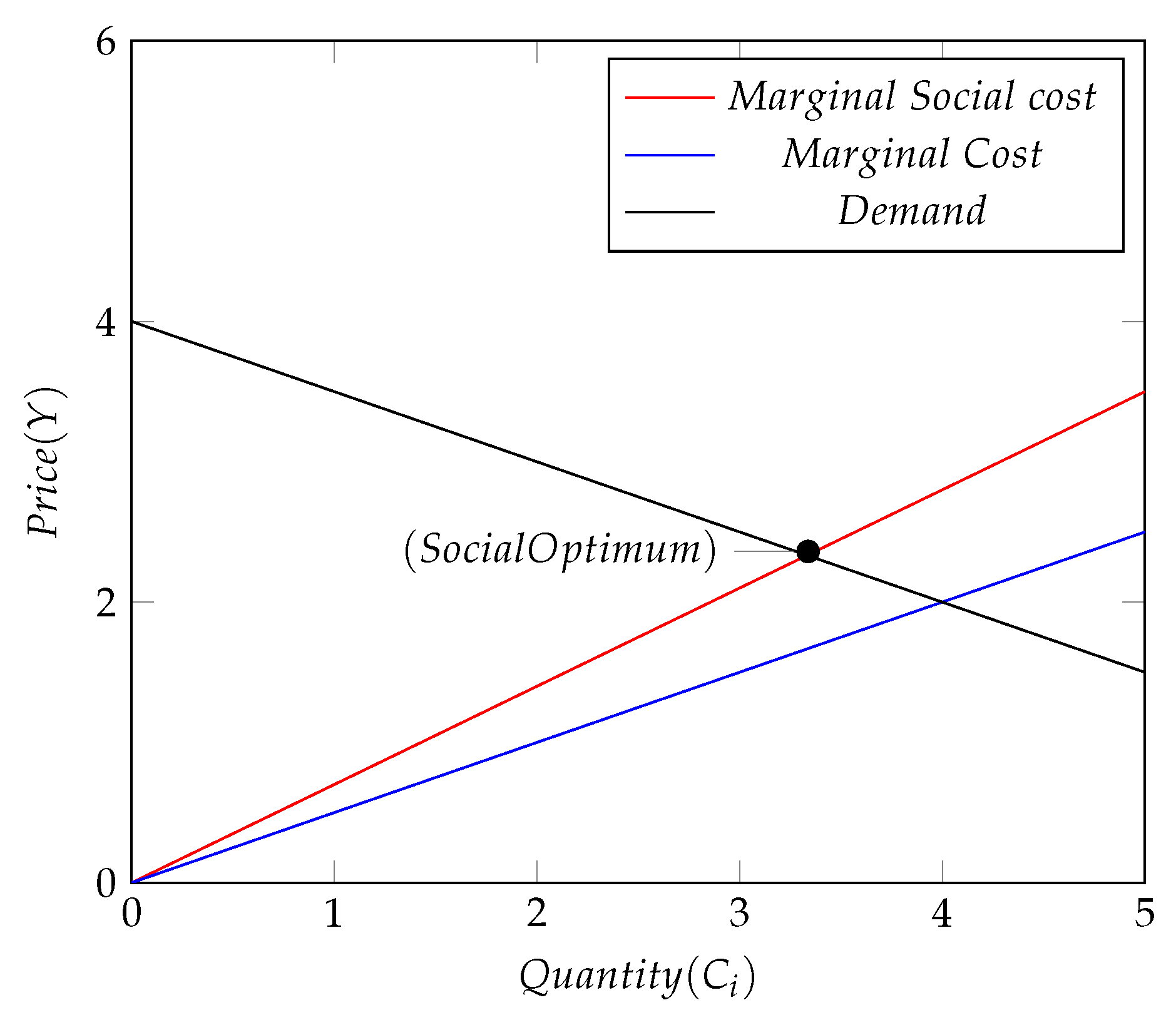
Appendix B.1. One Transaction

To introduce a Pigouvian applicative case, the following assumptions are needed. First, a hypothetical relation between price and quantity that considers the price to be a 1-1 monetary form of benefit is represented by a monotonically decreasing line. This assumption, together with the monotone constant increase to the marginal social cost MSi and the marginal production cost MCi, is arbitrarily set for the sake of understanding through a simple visual explanation. This demand is intrinsically related to the Utility (U), defined in Equation (1), and represents the stakeholder’s perceived benefit for the activity considered. The demand curve for the hypothetical considered good is described by the following arbitrary relation:
Y = α β C i α = 4 β = 0.5
Y is the demand and Ci is the quantity; let us proceed to identify the marginal production and social costs (MC and MS) stemming from the previous Equation (2). Let us proceed to substitute the value in (3) into the term E and consider that the activity does not require raw materials (e.g., the supplier does not have incoming transactions). Let us proceed to assume the marginal cost of the producer i (MCi, blue) for the production of the activity (the same can be done for a set of activities, with its resultant unit being a weighted average of the single entities) considered. The result will be the following:
M C i = E i = μ ϕ ψ C i
where Ci is the accounting unit in I.S.U. (International System of Units), and μ , ϕ , and ψ are, respectively, the efficiency of the energy processes of the producer, the compound exergy (or retrievable amount of work from the source material), and the energy price. Now let us consider the marginal cost of production as:
M C i = μ ϕ ψ C i = 0.5 C i
We can then assume and derive a hypothetical value for the μ , ϕ , and ψ (MCi):
μ = 0.5 ϕ = 1 ψ ψ = 0.25 EUR per kWh
Then, we assume the value for the price of carbon dioxide ( τ ) and its specific emission per quantity of output (pi) to be, respectively, EUR 28 per ton of CO2eq and 0.2/28 ton CO2eq per Kg. It follows that the impact cost per output of activity i is dependent on the specific materials required for the production of the energy necessary to produce the activity:
P i = τ p i C i = 0.2 C i
We can derive the resultant marginal social total cost by adding the cost of pollutants to the energetic cost of the activity. The marginal social cost plus the private cost curve (social total) are shown in the following equation (MSTi):
M S T i = E i + τ p i C i = 0.7 C i M S T i = M C i + M S i
Now, let us introduce the criterion that the producer would tend to maximize:
max C M B d C M C d C
which is the chosen amount of production C that defines the maximum of the revenue. This optimum will be a private (local) optimum because it does not yet include the externalities. By knowing also the criterion of the social authority (representing the whole set of stakeholders affected by this activity):
max C M B M S T d C
Solving graphically Equations (A6) and (A7), we get the respective private (local) and social (global) optimum, where the social optimum corresponds to a complete internalisation of the impact cost (MS). Particularly, its values are those of the following tuples of (C,Y) coordinates:
MC equilibrium : ( 4 , 2 ) MST equilibrium : ( 3 . 3 ¯ , 2 . 3 ¯ )
and a graphical representation is shown in the following plot:
Figure A1. Social optimum.
Applsci 13 06554 g0a1

Appendix B.2. Pigouvian Optimum in Real Case Scenario

The authority may proceed either to regulate quantities or prices. Let us consider it opts for price taxation. If emission and abatement costs were known for all stakeholders at transaction time t, then their information could be used to identify a better social optimum (considered as the internalization of all external costs, social cost, plus abatement cost). However, this is often not the case: considering a fixed tax T, this tax would be defined at the social equilibrium by having its value set as the value of the social cost non-internalized by the producer. Hence, a fixed tax inevitably implies non-efficient taxation of the externalities in the transitoriness of a production process because of the difference in marginal social costs (stakeholders may emit the same pollutant amounts but have different social costs (e.g., a factory in a populated centre versus the same or different factory in an industrial area)) for the same emissions and the stakeholders may have different abatement costs (access to different markets providing different abatement technology at different prices and efficiencies), but there also may be differences in demand and production costs (different utilities of goods in space and time and custom production features that make each production cost different among users along the time). Consider four stakeholders: A, B, C, D, with activities having demand, social cost, and private cost quantified according to the following scheme:
A
  • Total marginal cost: 0.8Ct
  • Marginal prod. cost: 0.5Ct
  • Marginal benefit (Price): 4 − 0.5Ct
B
  • Total marginal cost: 0.8Ct
  • Marginal prod. cost: 0.3Ct
  • Marginal benefit (Price): 4 − 0.1C3t
C
  • Total marginal cost 2 − 0.3Ct
  • Marginal prod. cost: 2
  • Marginal benefit (Price): 4 − 0.8Ct
D
  • Total marginal cost 1.2Ct
  • Marginal prod. cost: 0.6Ct
  • Marginal benefit (Price): 1 − 0.2C3t + C2t
Let us proceed to aggregate (this reasoning holds also for activities that are different for the audience reached, in its probability of purchase, and in the utilities to consumers, as well for different energetic costs, as it may be the case that there are different energy prices at different locations; it is valid as long as the variables of each activity are linearly independent from each other, e.g., social cost, production cost, abatement cost) them to obtain the resultant scenario for allowing the governmental authority to set its tax. Particularly, considering the demand, marginal social cost, and private cost curves as the sum of the four marginal social and private costs and demand for the goods resulting from A, B, C and D activities, the optimal tax to be chosen will be that value that minimizes the social costs while maximizing the benefits of the exchange. Thus, let us reintroduce the optimization criterion for obtaining the optimal social equilibrium for the governmental authority, as previously defined in Equation (A7):
arg max C M B M S T d C C * 3.08274421240038
By solving the maximization problem above, we get an optimal amount of Ct, which is approximatively equal to 3.08. Now let us substitute the social optimal quantity in the demand function. Given the marginal production cost (energetic cost) in line with the amount of the social optimum equilibrium being equal to:
A:
 1.54137210620019
B:
 0.924823263720113
C:
 2
D:
 4.00756747612049
The optimal Pigouvian tax, in the absence of information on abatement costs, can be deduced for each stakeholder as the difference between the price of the marginal benefit and the production curves, both evaluated at the social optimum amount previously discovered in Equation (A9):
A:
 0.917255787599622
B:
 0.14554876689045
C:
 −0.466195369920302
D:
 0.636488464188661
If any stakeholder has a positive impact, its taxation is considered as a subsidy and is represented with a negative sign. The optimal tax is different per each stakeholder because the sum of the marginal social cost and private cost of each stakeholder follows different patterns. Therefore, a fixed Pigouvian tax creates trade-offs among private stakeholders’ revenues and social optima proportional to the difference in patterns among the resultant total curves and the single stakeholder ones. Therefore, the standardisation introduced by a zero-order (constant) tax for all stakeholders would induce differences in the accounting of social effective costs due to a higher order of the social cost patterns of each stakeholder, i.e., due to different social costs occurring in different social contexts or locations (given the fact that impact for many polluting emissions depends on their dispersion and uptake into the ecosystem, the impact would be difficult to compensate for effectively. Moreover, the impact of the same pollutant could also depend on social conditions and behaviour, which are subjective and too complex for a proper accounting of without introducing further modelling on locations of emissions and pollutant dynamics).

Appendix B.3. Pigouvian Fixed Tax and Known Abatement Costs

Now let us consider a tax equal to the average tax among all four stakeholders previously introduced. Let the tax T be, therefore,
T 0.308
By knowing this time also the abatement cost each user has, the governmental authority may decide, once the tax T is set, to meter the achievement of its policies through the following indicator:
M S T a x ( C t C AB ) M C AB C AB d C
where MS stands for the marginal social cost, MCAB for the marginal abatement cost, and dCt and di, respectively, for the differential operator along amount C of activity i. Compared to the criterion previously defined, as in Equation (A7) or (A6), Equation (A10) is missing a term proper of a criterion; this is the reason why it is only an indicator of the attainment of the policies previously defined. The authority, once it has solved its first objective (A9) and set the optimal tax, does not have any role to intervene (unless with further additional policies). Let us now introduce the marginal abatement cost functions for the four considered stakeholders:
MCAAB:
        0.1Ct
MCBAB:
        0.3Ct
MCCAB:
        0 (does not emit the pollutant considered)
MCDAB:
        0.4 C2t
As the reader may point out, a given stakeholder, having a higher marginal abatement cost than the value of the tax, will convene to abate its impacts until the marginal abatement cost becomes greater than the value of the tax [44]. This phenomenon occurs because, once the amount of tax T is known, the producer benefit would be affected negatively either by the tax or by the abatement cost, given its criterion is still represented by Equation (A6) but this time with the subtraction of the term:
min ( T a x , M C A B )
where MCAB stands for the marginal cost of abatement for the considered amount of production C in the transitoriness. With the introduction of a fixed tax, the different abatement costs of each producer lead them to different strategies in the attainment of social equilibrium.
Considering the graphs in Figure A2, the reader can graphically see the amount each user would abate of the considered pollutant. This amount is expressed in relation to the units of the good produced, which, in this real-case scenario, has been assumed to be specific for each producer (through the term pi) and is expressed in relation to the output quantity Ct. The green line represents for each stakeholder the sum of its marginal abatement cost curve plus its marginal cost of production (energetic cost), and the dotted purple lines are its marginal cost curve (energetic cost) plus the tax introduced previously. The intersection of the purple line (dotted) with the green line represents the maximum amount that the user will find convenient to abate. By solving the maximization of the revenue for each stakeholder, and, once fixed, the total amount produced (amount at social optimum):
max C M B t M C t T a x ( C t C AB ) M C AB C AB d C
the amount CAB is found, which represents the quantity of abatement (always expressed as a function of the production of the good Ct considered). Particularly, for A, B, C, D, the chosen amount that maximizes each user’s revenue appears to be approximately equal to:
A
 3.08274420502072
B
 1.02758137221261
C
 0
D
 0.877887281291458
Figure A2. Pigouvian taxation in a real case scenario.
Applsci 13 06554 g0a2
As such, the Pigouvian tax still represents the achievement of a social Pareto optimal equilibrium in terms of Equation (A9), while in terms of minimization of abatement and social cost (introduced as the new social indicator in (A10)), the new target value after each stakeholder decides the amount to abate does not necessarily reach its optimum. As a result, non-compensated externalities occur proportionally to the deviation in value of the tax from the marginal social cost of each stakeholder i evaluated at its output amount Ct (at social equilibrium). Further, if abatement costs were known and integrated into (A9) in the evaluation of the optimum, the deviation among stakeholders would not allow the use of a fixed tax to abate all social costs. For this reason, a fixed tax can only aim at attaining the social optimal demand C through the abatement of social costs as long as the marginal abatement cost equals the fixed tax value (thus, a stakeholder may find it more convenient to pay the tax than to abate the emission). The abated amount can be increased by increasing the tax; nonetheless, its feasibility, in terms of modified output value for each stakeholder’s objective, will depend on the combination of the different abatement cost curves and social costs of the different stakeholders. Therefore, even when considering one single transaction, the fixed tax is a constant value, while the abatement costs in the transitoriness may have different patterns of higher or lower order. With a fixed tax rate, the tax payment exceeds the marginal damage cost for all units of output until the chosen abated quantity (the quantity at which marginal abatement costs become greater than the tax), causing an excess of total tax payment over total damage [44], which brings the user to quit the abatement, leading to lower values as indicated in Equation (A10).

Appendix B.4. Cap and Trade Market

Instead of considering the taxation as a price of the good, the authority may opt to tax the quantity of emissions. Knowing, therefore, the price of the pollutant for the criterion considered, we have previously introduced the price for the CO2eq in Equation (A4), which is equal to EUR 28/TonCO2eq.. The authority, once defining the global optimal amount at the social equilibrium (relative to the total amount of the four aggregated stakeholders, e.g., via Equation (A7)) decides to let the market self-regulate through the creation of vouchers that can be traded by those who feature lower emissions with respect to their allocated amount CALt. Therefore, the authority decides to opt for a strict egalitarian redistribution of the economic effort needed to achieve the social optimum amount. The authority sums all social costs of the four stakeholders and divides them by four, allocating to each of them an equal amount of the social cost. From previous simulation for the outcome of Equation (A9), the sum of social costs equal to (the social cost of the market (social cost curves of four stakeholders aggregated) divided the total amount of production is equal to the tax previously introduced) 3.80132473343553 with the tax per unit of Ctot equal to the previously defined tax. By so doing, each stakeholder is assigned a target amount to abate of
0.950331183358883
The different abatement costs of each producer lead them to different strategies in attaining the maximization of their revenue (which, at first approximation, let us consider to be dependent mainly on the differences in abatement costs); this creates a market for second-best attainment of the social optimum, which is driven by exchanges (trade) of allowances, having the resultant objective of keeping the total amount of emissions within the amount (cap, e.g., amount of emission at social optimum) chosen by the authority. In this particular case, given the abated amounts obtained from the previous section:
A
 3.08274420502072
B
 1.02758137221261
C
 0
D
 0.877887281291458
and calculating the effective social cost of each stakeholder at the social optimal amount (relative to the impact of the non-abated amount of emissions)
A
 0
B
 1.05592356733896
C
 −2.85099355007665
D
 1.45841821623506
Subtracting from it the share allowance in cost previously obtained, the resultant amount of money of each stakeholder either to be gained (−) or spent (+) through trading all allowances of abatement is equal to:
A
 0 − 0.950331183358883 = −0.950331183358883
B
 1.05592356733896 − 0.950331183358883 = 0.10559238398008
C
 −2.85099355007665 − 0.950331183358883 = −3.80132473343553
D
 1.45841821623506 − 0.950331183358883 = 0.508087032876176
Therefore, it follows that each user would be able to trade the above maximum amount of wealth (from reduced/increased emissions compared to its allocated amount of 0.950331183358883/tax). It follows that by dividing the costs above with the tax, the tradeable amount of each user is as follows:
A
 EUR −0.950331183358883/28 EUR TonCO 2 eq = −0.033940399405674 Ton CO2eq
B
 0.003771156570717 Ton CO2eq
C
 −0.135761597622698 Ton CO2eq
D
 0.018145965459864 Ton CO2eq
From the above values, you can also see how the cap-and-trade (fixed quantity) approach leads to inefficiencies in the abatement of all social costs. This effect is also due to the fact that even by acting on the total quantity Ctot at social optimum, this would not allow for considering differences in social costs induced by different impacts of the same pollutants emitted by different users. With the introduction of different abatement costs, the problem of abatement exit (defined in previous section) would also occur, therefore implying a non-optimal alternative as per criterion in Equation (A10). Moreover, compared to a price taxation, the creation of an emission market leads to further bias of accessibility and accountability. The profits generated out of the tax will no longer represent a governmental fund to mitigate the costs of the emission of third parties (not involved in the transaction), but rather it will represent an incentive for particular industrial strategies that (defined by particular social and abatement costs and technological scenarios) may favour particular industrial development strategies, especially under the influence of transnational corporations.
This might result in penalising the lower-middle-class citizens, who will make efforts to change their behaviour for producing sustainable outcomes whose benefits are claimable only by corporations; meanwhile their effects are not mitigated nor accounted for opportunely infra countries, knowing human life and natural capital have the same value at different locations. For instance, different health and safety laws for different countries imply different sampling and exposure standards, regardless of different estimates per each country provided by the IMF [45].

Appendix B.5. Scenario Comparison: The Decisional Problem

In this section, two variants are introduced to the four-stakeholder problem in the previous sections. The aim of this section is to highlight the Paretian decisional problem in terms of fulfilment of each stakeholder criteria (e.g., Equation (A6)) and social governmental criteria (e.g., Equation (A9)). The decisional problem is defined as following: knowing the amount of tax and the emission produced, each stakeholder modifies its abated amount CAB to maximize its own revenue, therefore influencing the governmental indicator defined in (A9). This problem has been simulated using Python’s Platypus library for multi-objective decisional problems, and its codebase implementation is hereby reported:
Listing A1. Problem initialization.
  • problem = Problem(4, 5, 9)
  • problem.types[:] = [Real(0, 3.08274420502072),
  •                                                   Real(0, 3.08274420502072),
  •                                                   Real(0, 1∗10∗∗(−10)),
  •                                                   Real(0, 3.08274420502072)]
  • problem.constraints[:] = “<=0”
  • problem.function = total_cost
  • problem.directions[:] = Problem.MAXIMIZE
  • algorithm = SPEA2(problem)
  • algorithm.run(1000)
where Problem(4,5,9) is used for initializing the problem class to solve a five-objective optimization problem subject to nine constraints and four decision variables. The Problem.MAXIMIZE function provides the criteria for the gradient to choose the next attempt of the dependent variable. With the maximization of a negative indicator being equal to the minimization of its respective positive amount, the constraints are considered negatively and their criterion set to lower than 0. This implies an abated amount between 3.08274420502072 and 0, with the sum of the four abated amounts by all stakeholders being lower or equal to 4 times 3.08274420502072. The algorithm used is SPEA2, and the cost function is: To answer the question of how the achievement of the social and individual objectives is influenced by a custom tax or by an authority that decides the amount of taxation including the abatement cost, the cost function defined above has been modified as later explained. In the following section, we will introduce different graphs to represent the Paretian decisional space, both in the alternative and objective space, as well in the overall achievement of the results.

Appendix B.5.1. Fixed Tax vs. Custom Tax

In case of custom taxes, the values to be compared are the outcome of the previous function defined in Listing A2 with the outcome of its new variant having different coordinates:
  •     tax = [0.91725579497928, 0.145548790143704,
  •               0.466195364016576, 0.636488470361734]
In the following graph, the feasible alternatives found are summarized, which have been filtered through Platypus from the Pareto dominated.
Figure A3. Social indicators (optimum in the alternative space—fixed vs. custom tax).
Applsci 13 06554 g0a3
Listing A2. Cost function.
  • def total_cost(va):
  •     x = va[0]; y = va[1]; z = va[2]; h = va[3]
  •     tax = [0.308274422867036, 0.308274422867036,
  •               0.308274422867036, 0.308274422867036]
  •     ctot = 3.08274420502072
  •     social = −tax[0]∗(ctot−x) \
  •                  −tax[1]∗(ctot−y)\
  •                  +tax[2]∗(ctot−z) \
  •                  −tax[3]∗ (ctot−h) \
  •                  − 0.1∗x∗∗2/2 − 0.3∗y∗∗2/2−0.4∗h∗∗3/3 \
  •                  − 1.4 ∗ ctot ∗ ctot /2 − 2 ∗ ctot \
  •                  + 13 ∗ ctot\
  •                  − 1.2 ∗ (ctot∗∗2) /2 \
  •                  + 1 ∗ (ctot∗∗3) /3 \
  •                  − 0.3 ∗ (ctot∗∗4)/4
  •     objectiveA = 4∗ctot −0.5∗(ctot∗∗2)/2 −0.5∗(ctot∗∗2)/2 \
  •                       − 0.1∗(x∗∗2)/2 − tax[0]∗(ctot−x)
  •     objectiveB = 4∗ctot−0.1∗(ctot∗∗4)/4 − 0.3∗(ctot∗∗2)/2 \
  •                       − 0.3 ∗ (y∗∗2)/2 \
  •                       − tax[1] ∗ (ctot−y)
  •     objectiveC = 4∗ctot \
  •                       − 0.8∗(ctot∗∗2)/2−2∗ctot\
  •                       −0.1∗(z∗∗2)/2 \
  •                       + tax[2]∗(ctot−z)
  •     objectiveD = ctot −0.2∗(ctot∗∗4)/4\
  •                       + (ctot∗∗3)/3 \
  •                       − 0.6∗(ctot∗∗2)/2 \
  •                       − 0.4∗(h∗∗3)/3 \
  •                       − tax[3]∗(ctot−h)
  •     constraints =  [x + y + z + h − ctot ∗ 4 ,
  •                       −x,
  •                       −y,
  •                       −z,
  •                       −h,
  •                       x−ctot ,
  •                       y−ctot ,
  •                       z−ctot ,
  •                       h−ctot]
  •     return [objectiveA,
  •              objectiveB,
  •              objectiveC,
  •              objectiveD,
  •              social], constraints
Particularly, we can notice how the algorithm converges to different alternatives of abated amounts for stakeholders A (circle), B (star), and D (triangle). In this graph, stakeholder C (square) has been neglected for the sake of representation and is not actually part of this decisional problem (choice of abated amount of emission) given its emissions are positive.
Figure A4. Trajectories of the decisional problem—fixed vs. custom tax.
Applsci 13 06554 g0a4
The blue and orange hues stand for the social objective result for both a custom-tax scenario and a fixed-tax scenario. The same alternatives can be represented in the space of objectives, having values represented by the Pareto border. Combining the two in Figure A5, we plot on the Y-axis the result of each private stakeholder’s objective (e.g., (A6)) and on the X-axis the abated amount of each stakeholder; the coloured bars represent achievement of the social optimum (Equation (A9)). It can be noticed how stakeholder C is the only one who benefits from the introduction of a custom tax. By introducing a custom tax, each stakeholder would not be induced to lower the choice of its abated amount, which would come at a cost proportional to its revenues.
Figure A5. Decisional scenario—fixed vs. custom tax.
Applsci 13 06554 g0a5

Appendix B.5.2. Influence of Information on Abatement Costs in the Decisional Process

Similar to what was previously done for identifying the differences between a custom and fixed Pigouvian taxation, a new comparison function is introduced. This new function has the total amount value equal to the quantity at the new social optimum equilibrium (Equation (A9)) obtained by using the information on abatement cost in the optimization criterion of the social optimum. Knowing the new total quantity Ctot of each stakeholder is equal to 2.43488451004777 as the result of Equation (A9), the new tax can be found, and the cost function can be modified accordingly:
  •     tax = [1.07984316017484, 1.07984316017484,
  •             1.07984316017484, 1.07984316017484]
  •     ctot = 2.43488451004777
Continuing, plotting the same graphs as in the previous section, it can be seen how the accounting of the abatement costs would induce a lower equilibrium, bringing further minimization of social costs but at an increasing price of each stakeholder’s revenue.
Figure A6. (a) Social indicators (fixed tax and custom tax) in the alternative space. (b) Decisional scenario.
Applsci 13 06554 g0a6
We invite the reader to see how the objective of C (square) increases compared to the custom tax, given its subsidy will increase. The stakeholders A (circle), B (star), and D (triangle) are those that will see their revenues reduced with an accounting of the abatement cost. Particularly, D will be the stakeholder that will be most affected, given its abatement costs increase with a higher order of magnitude compared to A or B. Moreover, it has been shown how the imposition of a tax created with the accounting of abatement costs may induce a lowering of the total social benefit overall, although Equation (A10) can be further optimized.

Appendix C. Transparency in Neofeudalism

In this section, we aim to put into context the usage of the protocol above. It is introduced to transparently and scientifically assess the dynamics of wealth generation involving landownership rights. In this context, particularly, we will disregard the influence capital polarization has in purchasing consensus for decision-making purposes, the scope of which is rather inherent in the structure itself of the energetic protocol previously introduced. Rather, the purpose of this section is to highlight the role of the distribution of land property rights.
Classical economists aimed to overcome the effects of the outweighing of wealth accumulation due to revenues from royalties over land ownership compared to labour income. This wealth, at that time accumulated by stakeholders called rentiers, occurred to be heritable, and so still is mostly worldwide.
Nowadays, although a century of economic development has passed, wealth from land royalties is still being concentrated at the vertix of the economic pyramid even though the feudal class evolved into postfeudal creditors. One of the reason that this wealth polarization occurred is the ability of stakeholders to inherit their wealth either from generation to generation or via sale of ownership with respective inheritance rights [46]. This phenomenon, as both Michael Hudson and Joel Kotkin highlighted, is not only related to ownership rights, but, currently, to a cooptation of interests between governments and speculators in the form of decision makers and capital owners as, for instance, is the case with real estate prices [46,47].
As previously mentioned, disregarding the dynamics regulating capital influence over decision making, we will focus on an oversimplified example to contextualise the sizes involved in the protocol introduced and to show how important it is to have a transparent understanding of wealth flow dynamics depending on the land-use planning and ownership rights. In this context, we will neglect the influence of Foreign Direct Investment FDI, for instance, operated by institutions such as the European Investment Bank (EIB). Through practices involving carbon offsetting and companies such as Ecosia, the influence of foreign capital flows plays a fundamental role, given the offsetting mechanism of CO2eq. influences land-use allocation with the risk of polarization of benefits by foreign stakeholders over satisfying local population needs, especially considering the involved non-governmental organizations harnessing local cheap labour, often in volunteer form. This situation is even more of a public concern when the organizations used as vehicles for Community (-based) Forestry CF policies are financed by taxpayers’ money from foreign countries, whose citizens are often completely uninformed of the risk of criminal practices of this new form of colonialism. Researchers have shown how Reducing Emissions from Deforestation and Degradation (REDD+) payments are not a comprehensive and holistically valid economic mechanism to address the diverse and competing interests of forest-dependent people and to compensate them adequately and equitably. In the worst cases, the implementation of CF policies has imposed added costs to the poor in terms of reduced access to forest products and forced allocation of household resources for communal forest management, implying insecurity over the benefits at the household level. As Mohan Poudel mentions, insufficient payment may not only be ineffective, but it may also be counterproductive [48].

Appendix C.1. Land-Use Allocation in Wealth Generation

For the purpose of having stakeholder interests more transparently identified and negotiated, the protocol defined in this paper was idealised. Therefore, let us consider a hypothetical case involving a land extension equal to 15 ha. This area is divided in three regions of equal size, each one having one decision-maker group, represented for the sake of simplicity by a single organization that represents the majority of the owners of the respective area. Each area consists of a population P, which is the same for each area and is equal to 500 people. Half of the population is not involved in any decision making or voting rights within the owner’s organization; indigenous people are an example of this, as they harness products from common land but lack legal claims over its ownership or its management, which may instead be assigned to a group of private stakeholders who benefit from concessions in land use. Further, let us consider a CF policy that aims at preserving the biosphere of all three areas, and in doing so, allows the managers and owners of the land to have control over the planning choice of resources producible on that land as long as they preserve vegetation, which is meant as governmental policy for CF. Let us further define three classes of production choices the landowners have: officinal plants (A), fruit trees (B), and wood houses (C). Each user group, for the sake of simplicity, is able to choose only one among the three planting alternatives A, B, or C for its whole area (50 km2). The average withdrawal of CO2eq is assumed to be 10 and 5 t o n h a y r for officinal plants and fruit, respectively. For wood houses, it can be considered as the carbon aerial intake of the primary resource used for their construction, which we will consider sourced from vegetation of a deciduous temperate forest with a rate equal to 20 t o n h a y r . Meanwhile, regarding the efficiency in the production of 1 Kg of products (e.g., officinal herb, fruit, or one house), let us suppose each officinal plant is able to produce 10 Kg of officinal herb, each fruit tree 15 Kg of fruit, and each biomass tree 20 kg of wood on average per year and per hectare, and let us hypothesize that the intraspecies competition of these different plants is the same, allowing for a maximum amount of 10,000 plants per hectare. Let us further consider the area has negligible rainfall compared to the amount of water required for growing the three different kinds of vegetation. This water is provided by a common water stream having a yearly renewed capacity of 5000 m3 of water from inflows external to the considered territory. From this water reservoir, each plant intake is 30, 40, or 50 m3 per year, respectively, for officinal, fruit, or biomass plants. Now let us introduce the exergy value of the primary common resource that all the three choices would need: water. Let us consider the exergetic value of water to be equal to 0.05 MJ/kg, which is also expressible as 0.013 8 ¯ kWh/kg. After that, let us assume that constructing wood houses is an output product of producing wood, which has, in terms of labour, a negligible amount of energy required for its creation, with the same reasoning used for its relative impact. Therefore, assume that both landowners and aborigens can build their own house from a certain biomass amount at a negligible cost. Or, similarly, assume that x value of biomass produced allows the building of a house of the same value. All sizes introduced are listed in Table A1.
Table A1. Variable set, units, and values for land-use implementation.
SymbolUnitValue50 km2, 1 yr
Tree DensityNo. of Plants/ha · yr10,000 5 × 10 7
RA* − YieldAkgofficinalis/plant10 5 × 10 8 Kg
RB* − YieldBkgfruit/plant15 7.5 × 10 8 Kg
RC* − YieldCkgbiomass/plant20 1 × 10 9 Kg
τ A | B | C EUR/tonCO228-
p A tonCO2/ Kg−0.2-
p B tonCO2/ Kg 0.0 6 ¯ -
p C tonCO2/ Kg−0.2-
CAtonCO2/m 2 yr−1 1 × 10 8 tonCO2
CBtonCO2/m 2 yr−0.5 5 × 10⁷ tonCO2
CCtonCO2/mm 2 yr−2 2 × 10⁸ tonCO2
μ A | B | C | C A | B | C H N %1-
ϕ A kWh/kg0.34 (24 h · 365 d)/10-
ϕ B kWh/kg0.34 (24 h · 365 d)/15-
ϕ C kWh/kg0.34 (24 h · 365 d)/20-
ψ A | B | C | C A | B | C H N EUR/kWh0.2-
R A C H N * m water 3 /plant30 1.5 × 10 9 m3
R B C H N * m water 3 /plant40 2 × 10 9 m3
R C C H N * m water 3 /plant50 2.5 × 10 9 m3
ϕ C A | B | C H N kWh/kg 0.014 8 ¯ -

Appendix C.1.1. Evaluating Objective Wealth

Let us now consider that landowners would tend to optimize their subjective wealth, expressed by Equation (3). We can write the yearly wealth balance for the three user groups of the three respective areas having equal geographic extension and similar physical properties as the following:
O U G = C A | B | C H N + E A | B | C
Consider any of the three areas of 5000 ha of extension and a single transaction in the time interval t t 0 of 1 year. The equation above can be written as following considering the stakeholder committee decides to produce product A:
O U G = μ C A H N · ψ C A H N · ϕ C A H N · R A C H N + μ A · ψ A · ϕ A · R A O U G = 1 × 0.2 × 0.014 8 ¯ × 1.5 × 10 9 + 1 × 0.2 × 297.64 × 5 × 10 8 = EUR 2.976 × 10 10
In case the product decided to be produced is product B, the previous equation assumes the following value:
O U G = μ C B H N · ψ C B H N · ϕ C B H N · R B C H N + μ B · ψ B · ϕ B · R B O U G = 1 × 0.2 × 0.014 8 ¯ × 2 × 10 9 + 1 × 0.2 × 198.56 × 7.5 × 10 8 = EUR 2.978 × 10 10
Instead, for product C, we can write the following:
O U G = μ C C H N · ψ C C H N · ϕ C C H N · R C C H N + μ C · ψ C · ϕ C · R C O U G = 1 × 0.2 × 0.014 8 ¯ × 2.5 × 10 9 + 1 × 0.2 × 148.92 × 1 × 10 9 = EUR 2.979 × 10 10
As we can see from the above wealth generation values, in this fictitious example, the activity that creates most of the value involves the production of biomass. This is due to the increased amount of water exploited for the production of the so-created product and its higher yield per unit of area (the same plants have the same maximum density per unit of area). This result represents the produced wealth of the three economic activities from the resources they harness; however, it is meaningless in terms of added wealth to stakeholders unless we consider a transaction counterparty, and therefore the benefit and relative utility that the buyer would have in such a produced good. The higher the benefit for the buyer, the higher the profit would be for the producer in the sale of such produced goods. Thus, the last assumption needed is the utility value the different producible goods have for the population. For sake of simplicity in the understanding, we will be considering the utility as a one-to-one monetary form of the benefit of constant value per output amount and equal among landowner and aborigen categories, as defined in Table A2:
Table A2. Benefits of stakeholders from activities.
Stakeholdersf(UA)f(UB)f(UC)
user groupsEUR 10EUR 1EUR 2
AborigensEUR 4EUR 2EUR 1
Further, let us assume both groups are not limited by any account balance restriction in achieving their needs, and that during a year, each stakeholder of both groups aims at satisfying the whole demand of produced goods in the whole area during a year. We will neglect the study of the sizes involved among users of the same group. The example we discuss aims at providing insights on how to apply the protocol to wealth generation from land-use allocation dynamics.

Appendix C.1.2. Evaluating Subjective Wealth

To this purpose, let us now proceed to apply both Equations (7) and (12) as planning tools for the landowners to decide which choice among the producible output can maximize their revenue. For Equation (7), we can write:
O U G = 250 × ( 10 + 4 ) × 5 × 10 8 μ C A H N · ψ C A H N · ϕ C A H N · R A C H N + μ A · ψ A · ϕ A · R A = 1.75 × 10 12 2.976 × 10 10 EUR 1.720 × 10 12
Continuing for product B:
O U G = 250 ( 1 + 2 ) × 7.5 × 10 8 μ C B H N · ψ C B H N · ϕ C B H N · R B C H N + μ B · ψ B · ϕ B · R B = 5.625 × 10 11 2.978 × 10 10 EUR 5.327 × 10 11
While for product C:
O U G = 250 × ( 2 + 1 ) × 10 9 μ C C H N · ψ C C H N · ϕ C C H N · R C C H N + μ C · ψ C · ϕ C · R C = 7.5 × 10 11 2.979 × 10 10 EUR 7.20 × 10 11
From the results above, we can see that in the considered area, the first product would be more profitable for the stakeholders of the user group landowners. Nonetheless, this would create a penalising situation for aborigens that will see their wealth decrease relative to their initial wealth and compared to that of the landowners; it is proportional to the difference in the utilities the two groups have: f ( U A | B | C U G ) f ( U A | B | C N o n U G ) for equal production cost.

Appendix C.1.3. Including Impacts

Let us rewrite the above equations for the user groups now including the impact term we quantified in Table A1.
Again for product B:
O U G = 250 ( 1 + 2 ) × 7.5 × 10 8 + 28 × 5 × 10 7 μ C B H N · ψ C B H N · ϕ C B H N · R B C H N + μ B · ψ B · ϕ B · R B = 5.625 × 10 11 2.978 × 10 10 EUR 5.341 × 10 11
Finally, for product C:
O U G = 250 × ( 2 + 1 ) × 10 9 + 28 × 2 × 10 8 μ C C H N · ψ C C H N · ϕ C C H N · R C C H N + μ C · ψ C · ϕ C · R C = 7.5 × 10 11 2.979 × 10 10 EUR 7.258 × 10 11

References

  1. Quesnay, F. Tableau Oeconomique; Macmillan: New York, NY, USA, 1894. [Google Scholar]
  2. Cobb, C.W.; Douglas, P.H. A theory of production. Am. Econ. Rev. 1928, 18, 139–165. [Google Scholar]
  3. Coase, R.H. The problem of social cost. In Classic Papers in Natural Resource Economics; Springer: Berlin/Heidelberg, Germany, 1960; pp. 87–137. [Google Scholar]
  4. Pigou, A.C. The Economics of Welfare; Palgrave Macmillan: London, UK, 2013. [Google Scholar]
  5. Baumol, W.J. Leontief’s great leap forward: Beyond Quesnay, Marx and von Bortkiewicz. Econ. Syst. Res. 2000, 12, 141–152. [Google Scholar] [CrossRef]
  6. Frischknecht, R. Transparency in LCA-a heretical request? Int. J. Life Cycle Assess. 2004, 9, 211–213. [Google Scholar] [CrossRef]
  7. Fritter, M.; Lawrence, R.; Marcolin, B.; Pelletier, N. A survey of Life Cycle Inventory database implementations and architectures, and recommendations for new database initiatives. Int. J. Life Cycle Assess. 2020, 25, 1522–1531. [Google Scholar] [CrossRef]
  8. Wittmaier, M.; Langer, S.; Sawilla, B. Possibilities and limitations of life cycle assessment (LCA) in the development of waste utilization systems-Applied examples for a region in Northern Germany. Waste Manag. 2009, 29, 1732–1738. [Google Scholar] [CrossRef] [PubMed]
  9. Howard, N. Environmental assessment and rating-have we lost the plot? Procedia Eng. 2017, 180, 640–650. [Google Scholar] [CrossRef]
  10. Leontief, W. Environmental repercussions and the economic structure: An input-output approach. Rev. Econ. Stat. 1970, 52, 262–271. [Google Scholar] [CrossRef]
  11. Hendrickson, C.; Horvath, A.; Joshi, S.; Juarez, O.; Lave, L.; Matthews, H.S.; McMichael, F.C.; Cobas-Flores, E. Economic Input-Output-Based Life Cycle Assessment (EIO-LCA). Mental 1998. Available online: https://www.researchgate.net/profile/H-Matthews-2/publication/242142910_Economic_Input-Output-Based_Life-Cycle_Assessment_EIO-LCA/links/0c96053b2c2bd76615000000/Economic-Input-Output-Based-Life-Cycle-Assessment-EIO-LCA.pdf (accessed on 23 May 2023).
  12. Troszak, T. Why do we burn coal and trees to make solar panels? Res. Gate 2019. [Google Scholar] [CrossRef]
  13. Remme, R.P.; Edens, B.; Schroter, M.; Hein, L. Monetary accounting of ecosystem services: A test case for Limburg province, the Netherlands. Ecol. Econ. 2015, 112, 121. [Google Scholar] [CrossRef]
  14. Ruet, J.; Gambiez, M.; Lacour, E. Private appropriation of resource: Impact of peri-urban farmers selling water to Chennai Metropolitan Water Board. Cities 2007, 24, 110–121. [Google Scholar] [CrossRef]
  15. Neir, A.M. The history of the Federal government’s involvement in water resources: An attempt to correct externalities? Water Resour. Prof. Proj. Rep. 2010, 12–13. Available online: https://digitalrepository.unm.edu/cgi/viewcontent.cgi?article=1140&context=wr_sp (accessed on 23 May 2023).
  16. Chiolerio, A. Liquid Cybernetic Systems: The Fourth-Order Cybernetics. Adv. Intell. Syst. 2020, 2, 2000120. [Google Scholar] [CrossRef]
  17. Solid Biomass Conformity Assessment Scheme for Energy Applications. Available online: https://wetten.overheid.nl/BWBR0040431/2018-01-01/ (accessed on 23 May 2023).
  18. Murray, D.; Stankovic, L.; Stankovic, V.; Espinoza-Orias, N. Appliance electrical consumption modelling at scale using smart meter data. J. Clean. Prod. 2018, 187, 237–249. [Google Scholar] [CrossRef]
  19. Pratt, R.G.; Balducci, P.J.; Gerkensmeyer, C.; Katipamula, S.; Kintner-Meyer, M.C.; Sanquist, T.F.; Schneider, K.P.; Secrest, T.J. The Smart Grid: An Estimation of the Energy and CO2 Benefits; Technical Report; Pacific Northwest National Lab. (PNNL): Richland, WA, USA, 2010. [Google Scholar] [CrossRef]
  20. Toma, A.R.; Gheorghe, C.M.; Neacsu, F.L.; Dumitrescu, A.M. Conversion of smart meter data in user-intuitive carbon footprint information. In Proceedings of the 2017 5th International Symposium on Electrical and Electronics Engineering (ISEEE), Galati, Romania, 20–22 October 2017; IEEE: Piscataway, NJ, USA, 2017; pp. 1–6. [Google Scholar] [CrossRef]
  21. Taranto, F. Exergy Indicators for Resource Impact Assesment: An Application of Erosion Remediation Techniques on Highway Slope. POLITesi 2013. Available online: https://www.politesi.polimi.it/handle/10589/75062 (accessed on 23 May 2023).
  22. Cochrane, D.; Hammarfelt, B.; Rushforth, A.D.; de Rijcke, S.; Chong, P.K.; Bourgoin, A.; Meyer, M.; Wilbanks, R.; Bidet, A. Disobedient Things: The Deepwater Horizon Oil Spill and Accounting for Disaster. Valuat. Stud. 2020, 7, 3–32. Available online: https://valuationstudies.liu.se/article/download/357/1023 (accessed on 23 May 2023). [CrossRef]
  23. Hennings, K.H. Capital as a Factor of Production. In Capital Theory; Springer: Berlin/Heidelberg, Germany, 1990; pp. 108–122. [Google Scholar]
  24. Serrano, F.; Mazat, N. Quesnay and the Analysis of Surplus in the Capitalist Agriculture. Contrib. Political Econ. 2017, 36, 81–102. [Google Scholar] [CrossRef]
  25. Nitzan, J.; Bichler, S. Capital as Power: A Study of Order and Creorder; Routledge: London, UK, 2009. [Google Scholar]
  26. Alessio, F.J. Energy analysis and the energy theory of value. Energy J. 1981, 2. [Google Scholar] [CrossRef]
  27. Chen, J. An entropy theory of value. Struct. Chang. Econ. Dyn. 2018, 47, 73–81. [Google Scholar] [CrossRef]
  28. Costanza, R. Value theory and energy. Encycl. Energy 2004, 6, 337–346. [Google Scholar]
  29. Sciubba, E. From Engineering Economics to Extended Exergy Accounting: A Possible Path from Monetary to Resource-Based Costing. J. Ind. Ecol. 2004, 8, 19–40. [Google Scholar] [CrossRef]
  30. Stallinga, P. On the Energy Theory of Value: Economy and Policies. Mod. Econ. 2020, 11, 1083–1120. [Google Scholar] [CrossRef]
  31. Hyman, E. Net Energy Analysis and the Theory of Value: Is It a New Paradigm for a Planned Economic System? East-West Center: Honolulu, HI, USA, 1980. [Google Scholar]
  32. Szargut, J. Analysis of cumulative exergy consumption. Int. J. Energy Res. 1987, 11, 541–547. [Google Scholar] [CrossRef]
  33. Ayres, R.U.; Van den Bergh, J.C. A theory of economic growth with material/energy resources and dematerialization: Interaction of three growth mechanisms. Ecol. Econ. 2005, 55, 96–118. [Google Scholar] [CrossRef]
  34. Lindsey, R. Climate and Earth’s Energy Budget. NASA-Earth Obs. 2019. Available online: https://earthobservatory.nasa.gov/features/EnergyBalance (accessed on 23 May 2023).
  35. Brown, N. Contradictions of value: Between use and exchange in cord blood bioeconomy. Sociol. Health Illn. 2013, 35, 97–112. [Google Scholar] [CrossRef]
  36. Delgado-Galvan, X.; Perez-Garcia, R.; Izquierdo, J.; Mora-Rodriguez, J. An analytic hierarchy process for assessing externalities in water leakage management. Math. Comput. Model. 2010, 52, 1194–1202. [Google Scholar] [CrossRef]
  37. Szargut, J.; Morris, D.R. Cumulative exergy consumption and cumulative degree of perfection of chemical processes. Int. J. Energy Res. 1987, 11, 245–261. [Google Scholar] [CrossRef]
  38. Garofalo, E.; Bevione, M.; Cecchini, L.; Mattiussi, F.; Chiolerio, A. Waste Heat to Power: Technologies, Current Applications, and Future Potential. Energy Technol. 2020, 8, 2000413. [Google Scholar] [CrossRef]
  39. He, W.; Kong, X.; Qin, N.; He, Q.; Liu, W.; Bai, Z.; Wang, Y.; Xu, F. Combining species sensitivity distribution (SSD) model and thermodynamic index (exergy) for system-level ecological risk assessment of contaminates in aquatic ecosystems. Environ. Int. 2019, 133, 105275. [Google Scholar] [CrossRef]
  40. Chanel, O.; Douenne, T.; Lefèvre, M. Valuing the Economic Consequences of Air Pollution-Related Health Risks: A Review of Recent Studies. Int. J. Environ. Res. Public Health 2019, 16, 2373. [Google Scholar] [CrossRef]
  41. De Meester, B.; Dewulf, J.; Janssens, A.; Van Langenhove, H. An improved calculation of the exergy of natural resources for exergetic life cycle assessment (ELCA). Environ. Sci. Technol. 2006, 40, 6844–6851. [Google Scholar] [CrossRef]
  42. Bosch, M.E.; Hellweg, S.; Huijbregts, M.A.; Frischknecht, R. Applying cumulative exergy demand (CExD) indicators to the ecoinvent database. Int. J. Life Cycle Assess. 2007, 12, 181. [Google Scholar] [CrossRef]
  43. Castano, S.; Sanz, D.; Gomez-Alday, J.J. Methodology for quantifying groundwater abstractions for agriculture via remote sensing and GIS. Water Resour. Manag. 2010, 24, 795–814. [Google Scholar] [CrossRef]
  44. Burrows, P. Pigovian Taxes, Polluter Subsidies, Regulation, and the Size of a Polluting Industry. Can. J. Econ. 1979, 12, 497–499. [Google Scholar] [CrossRef]
  45. Parry, I.W.; Heine, M.D.; Lis, E.; Li, S. Getting Energy Prices Right: From Principle to Practice; International Monetary Fund: Washington, DC, USA, 2014. [Google Scholar]
  46. Hudson, M. The Road to Debt Deflation, Debt Peonage, and Neofeudalism; Number 708, Working Paper; Levy Economics Institute of Bard College: Annandale-On-Hudson, NY, USA, 2012. [Google Scholar]
  47. Kotkin, J. The Coming of Neo-Feudalism: A Warning to the Global Middle Class; Encounter Books: New York, NY, USA, 2020. [Google Scholar]
  48. Poudel, M. Examining Outcomes of REDD+ through Community Forestry in Rural Nepal. Ph.D. Thesis, Institute of Forestry, Tribhuvan University, Kirtipur, Nepal, 2014. [Google Scholar]
Figure 1. System boundaries and energy and information flows.
Applsci 13 06554 g001
Figure 2. Protocol gate-to-gate diagram.
Applsci 13 06554 g002
Figure 3. Interaction of stakeholders in a simplified supply chain sub-system.
Applsci 13 06554 g003
Table 1. EPD categories.
CriterionUnit
AcidificationKg SO2eq
EutrophicationKg PO4-eq
Global warmingKg CO2eq
Depletion of stratospheric ozone layerKg CFCeq
Formation of tropospheric ozoneKg Ethyleneeq
Table 2. Variables and units.
SymbolUnit
tStakeholder
NThreshold
jSupplier
Oi,j
Ei,j
Ci,jKg or m3 s.c.
Pi,j
pi,jStandardised impact
unit (S.I.U.)/Kg
Table 1; Section 3.4
Disclaimer/Publisher’s Note: The statements, opinions and data contained in all publications are solely those of the individual author(s) and contributor(s) and not of MDPI and/or the editor(s). MDPI and/or the editor(s) disclaim responsibility for any injury to people or property resulting from any ideas, methods, instructions or products referred to in the content.

