On Fuzzy and Case-Based Dynamic Software Development Process Modeling and Simulation Approach

Abstract

The software development process (SDP) is complex because it uses specific knowledge, skills, tools, and techniques to deliver value to people, and the user’s needs are always growing and becoming more complex. Practitioners and academics have proposed different approaches for improving the successful implementation of the SDP. This remains a non-trivial task, and the number of successful software development projects increases only slightly each year. This paper proposes a new approach for adapting the classical SDP to a dynamic, knowledge-intensive, and context-dependent model by applying the case-handling and fuzzy inference approaches for SDP modeling and simulation. The advantages and novelties of this approach consist in: SDP dynamicity modeling using the case-handling approach; the inclusion of human factor uncertainty into the execution of SDP activities through fuzzification; and agent-based simulation, which allows for the inclusion of human actors in SDP simulations. Modeling and simulation of Agile SDPs were carried out using this prototype. Experiments show the correspondence of the proposed approach to the needs of dynamically changing and human-factor-dependent SDPs, as well as the possibilities for modeling and simulating the SDP, predicting SDP execution, and observing possible risks.

1. Introduction

The software development process (SDP) is complex, dynamic [1], and knowledge-intensive [2] by its nature, and it is affected by a dynamically changing environment. Examples of such dynamic changes of environment include regulatory adaptations (e.g., changes in raw material prices), market evolution (e.g., stock price change), changes in customer behavior (e.g., rapid change in customer needs), process improvement, and policy shifts and exceptions.

Existing approaches used to model, simulate, and adopt SDPs with regard to these changes insufficiently cover the actual needs of businesses. Increasing numbers of authors are discussing the inadequate planning that causes the failure of software projects [3]. The reasons for these failures are investigated via different approaches. Some authors have already investigated possible influential factors in Agile or other software projects. For example, [4] emphasized such factors as national culture, organizational culture, and collaborative work environment as being influential regarding Agile adoption. Meanwhile, [5] considered the social and human factors that impact SDP and productivity. Their research was based on a survey and aimed to gather information on the perceptions of software development teams regarding the social factors that influence productivity. This information was then compared with the different variables of the software developers themselves. From this perspective, social and human factors play a significant role in the SDP and can influence the performance of the development team [6,7]. Those factors can be considered characteristics of an individual based on their behaviors from both a social and individual perspective.

This also can be seen from the Chaos Report [8], which indicates that the number of successful projects increases slightly from year to year [9].

Thus, there is a need in the area of SDP simulation, which allows us to view the SDP as a dynamic and knowledge-intensive business process (BP) that is highly dependent on human factors and business needs.

In the literature, different BP modeling techniques can be observed based on different viewpoints. The most widely known are: (1) Business Process Modeling Notation (BPMN) [10]; (2) a flow chart [10]; (3) a Petri Net [10]; (4) rich pictures [11]; and (5) a Gantt chart [11].

However, since the SDP does not require a strictly predefined process flow, instead requiring that employees have access to all of the information relevant to a particular case and the freedom to make decisions [12], a case-handling approach is appropriate for this kind of process modeling. This approach also focuses on what can be done to achieve a predefined process goal rather than using a predefined workflow of the process that corresponds to the Agile work principle [13]. A case-handling approach is implemented in the Case Management Model and Notation (CMMN) [13].

Fuzzy logic offers a useful approach when modeling application domains requiring the incorporation of subjective information and significant uncertainties [14]. This approach is already used for software cost estimation, when solving the software effort estimation problem [15], or to make decisions in information security management for software-defined networks. The human factor (HF) is becoming a thoroughly discussed topic in different subject areas as it has a significant influence on different processes. Because calculating and predicting the influence of the HF is difficult and can differ according to subject areas, in this research we are going to use fuzzy logic to express HFs when simulating the SDP.

Simulation in various complex BPs is already applied by organizations seeking to optimize long-established workflows [16]. BP simulation allows process executors to see a complete picture of the simulated process (i.e., the interdependencies of activities, the conditions for the execution of activities, and possible crashes or downtime locations). SDP simulation can help to plan the SDP and reduce its chance of failure. However, SDP simulation is insufficient and lacks both theoretical and practical components. Current BP modeling and simulation techniques are suitable for the modeling and simulation of a static BP and can precisely predict which activities to execute and in what order. The bulk of present tools and techniques demand extremely tight BP specification, and unanticipated BP activity sequences cannot be included during BP execution [1].

Consequently, the main aim of this paper is to propose an approach to fuzzy and case-handling-based dynamic SDP modeling and simulation. For the sake of clarity, the Agile SDP management methodology is chosen for research in this paper.

The main scientific contributions of this paper are as follows:

• A new, fuzzy, case-handling-based dynamic SDP modeling and simulation approach is proposed, which allows us to predict the SDP in terms of its resources, task execution time, and sequence of tasks.
• The proposed approach to fuzzy and case-handling-based dynamic SDP modeling and simulation is applicable for: (1) dynamic SDP through application of the case-handling approach; (2) understanding the impact of the HF through fuzzification; and (3) using an adaptive neuro fuzzy inference system (ANFIS) to achieve more precise simulation results.
• The proposed fuzzy and case-handling-based dynamic SDP modeling and simulation approach is implemented as an automatic SDP simulation, employing both the CMMN model and ANFIS.
• The proposed fuzzy and case-handling-based dynamic SDP modeling and simulation approach was applied to a particular SDP management method: Agile.

The novelty of the current research is the combination of fuzzy inference applying ANFIS with case-based process modeling using CMMN into one simulation model.

This study contributes to SDP research by: investigating BP modeling approaches suitable for the SDP; adopting CMMN for dynamic and knowledge-intensive BP; and analyzing the impact of HF on SDP execution. Moreover, the results of this study allow the authors to precisely predict possible deviation and to reduce possible risks in the SDP.

This paper is intended to assist researchers and practitioners working on software implementation projects. The practical utility of this paper is that it familiarizes researchers and practitioners with the key properties of the SDP, enabling their application in order to enhance the success of software implementation projects. This results in a more complete picture of the SDP during the simulation process.

The rest of the paper is organized as follows: Section 2 describes preliminaries; Section 3 reviews the literature on SDP; Section 4 describes the approach of this research; Section 5 presents a case study and the results of an experimental study by using SDP modeling and simulation; and, finally, Section 6 and Section 7 conclude the paper.

2. Preliminaries

The SDP is the process of developing a software product. In general, it includes most development processes and makes use of the following activities: requirement gathering, design, implementation, testing, and maintenance [17].

The Agile approach is an iterative method of project management and software development that supports teams in providing value to their clients more rapidly and efficiently. Agile approaches in software development include: requirement discovery and solution improvement through cooperative work with end users by self-organizing, cross-functional teams; adaptive planning; evolutionary development; early delivery; ongoing improvement; reactions that are able to adapt to changes in needs and capacity; and understanding the problems to be solved [18].

A dynamic business process (DBP) is a process that supports structural and functional changes (i.e., has no predefined activities nor sequence of activities) during the DBP instance run-time according to its context and rules and that can be implemented with minimal delay [19].

CMMN is known for its adaptive approach to case management, which assists in decision making by making suggestions and retaining people in management positions. In contrast to the workflow-based approach, which uses a control flow to describe the process, case management is concerned with providing data and information about the process case to the workers [13].

A fuzzy set—A, in the example below—is a set where each of the elements have degrees of membership [20]:

$$A=\{u, {\mu }_A\left(u\right)|u\in U, {\mu }_A: U\to \left[0;1\right]\}$$

where A is in the universe of discourse U, and µ_A(u) is a membership function (MF) of u in A. The value µ_A(u) represents the grade of membership of u in A and is interpreted as the degree to which u belongs to A.

3. Related Works

Because software has been a critical part of the global economy for a considerable length of time, many authors have already analyzed possible approaches to SDP modeling. In [21], the authors compared seven different development models: waterfall, iterative, spiral, V-shape, incremental, RAD, and Agile. They considered and compared different software development models, focusing more on the management of software development modeling (i.e., how software development is divided into stages and in which order it should be conducted).

As was observed in the introduction, the SDP is dynamic, flexible, and knowledge intensive. In this section, we provide an overview of approaches to modeling such processes. In a previous paper, we analyzed BPs and approaches to their modeling according to SDP requirements [22]. This involved the search for another perspective from which to compare existing types of BP modeling and find the approach most suitable to the software development subject area. The results of this comparison show us that the BP modeling approach most suitable for the SDP is case handling, as it meets all of the defined requirements for the SDP. Moreover, it focuses on what can be done to achieve a predefined process goal rather than using a predefined workflow.

CMMN provides greater flexibility and features in order to represent work on task lists [23]. Work can be organized in phases with different semantic execution. Tasks in work can be optional, and their potential sequence of execution does not need to be explicitly modeled—only a particular criterion for routing among tasks needs to be provided. However, this CMMN-based modeling may require more domain analysis than the same process specified in a BPMN model. CMMN also supports elements for goal-driven and declarative modeling [23]. Thus, by adapting CMMN and assessing the scope, resources, and risks of a future SDP, the probability of SDP failure can be reduced [13]. CMMN is already used to model DBPs. In [24], the authors set the goal of examining whether CMMN could be effectively used to model social processes. Their research proposed an extension to case management by infusing social characteristics into the methodology of adaptive case management [24]. The authors proved that the alteration of adaptive case management, supported by CMMN, is effective in modeling human-intensive processes—especially when executable CMMN models are automated and executed within social environments.

CMMN is designed to capture common elements used by the case management of the same product. CMMN is known for its adaptive case management, which assists in decision making by making suggestions and keeping people in managerial positions. The case management approach provides workers with data and information about a case in order to give them control regarding how a case runs [12]. The case model is focused on real, rapidly changing information and relationships, while traditional BPs are focused on predefined sequences of activities [12]. CMMN is declarative, meaning what can and cannot be done in a process is described; meanwhile, BPMN is imperative, meaning how a process can proceed is described [12]. The main difference between this and other Object Management Group (OMG) (https://www.omg.org/, accessed on 5 December 2022) notations is that in the case management system, workers are responsible for business goals (i.e., the system is only a tool to achieve these goals) [12]. It could also be said that CMMN and BPMN represent a shift from procedural to declarative models [25]. CMMN is commonly used to model dynamic processes, and increasing numbers of tools are now emerging that allow models to be run and integrated with other tools. The case model shows all tasks and their execution parameters, which shows that these tasks can be performed inconsistently—some tasks can be commenced during the execution of other tasks if there are sufficient free resources in the same time interval [26]. One of the main advantages of CMMN is that it provides the opportunity to illustrate discrete events, thus allowing case handlers to decide for themselves whether a task is relevant to the execution process and whether it will be executed [25]. It was observed as early as 2013 that CMMN could provide a suitable opportunity to identify and model dynamic processes. CMMN proposes that users move away from traditional process flow modeling and start to use task sets that can be commenced dynamically once the entire process begins [27].

There are already some methods suggested in related works that could help improve project management or software development in various organizations. For example, the Constructive Cost Model (COCOMO) helps to estimate software cost and quality, analyze risk, and so on [27], and was built based on 63 software projects [27]. COCOMO also has its disadvantages, such as its ignorance of requirements and documentation, hardware issues, personnel turnover levels, and its dependence on the amount of time spent on each phase [28]. Therefore, different model extensions are proposed, such as COCOMO-Fuzzy [29], which applies a neuro-fuzzy approach to retain some desirable fuzzy features, including learning ability and good interpretability, while maintaining the merits of the COCOMO model. The model effectively deals with imprecise and uncertain input and enhances the reliability of software cost estimates. In addition, it allows inputs to have continuous rating and linguistic values, thus avoiding similar projects having high variance in estimated costs [29].

Another famous simulation method is Monte Carlo [30], which relies on repeated random sampling and statistical analysis to compute results. This method is considered appropriate for “what-if” analysis [30]. In addition, it is a direct method for performing both simulation and integration [31]. The main disadvantage of the traditional Monte Carlo method is that it is suitable for static data only (i.e., it is not suitable for run-time adaptations during simulation); moreover, it is difficult to conduct large-scale maneuvers in Monte Carlo [32]. The Monte Carlo method is also integrated with fuzzy logic [33]. Some authors [33] have proposed a method that provides a better measure of uncertainty than existing methods (i.e., unlike the traditional risk analysis method). This approach considers both the variability and uncertainty of information in risk calculation; instead of a single risk value, interval risk values are provided for a given percentile of risk.

In [34], the authors suggested using the Integrated Business IT Impact Simulation (IntBIIS) approach to adequately reflect the mutual impact between BPs and information systems (IS) in simulation. This approach is implemented by extending the Palladio tool chain with BP simulation concepts [34]. IntBIIS predicts the impact of IS design and BP performance. The main disadvantage of the suggested approach is that the HF (stress level, motivation, experience, etc.) is not considered. This method is also more suitable for the simulation of a basic BP, but not a dynamic and complex BP management process that has various additional sub-processes.

Other authors have already used machine learning methodologies for optimizing and modelling processes in different domains. For example, the authors in [35] use machine learning for engineering challenges in non-linearity and complexity areas. Other authors in [36] use data-driven machine learning techniques for forecasting thermophysical features and heat transfer rate. The authors reviewed literature to highlight the current advances in machine learning for their domains. They concluded that machine learning techniques can accurately predict nanofluid characteristics.

In [37], the author observed that there is no standard model for BP simulation; they differ because of the chosen software development methodologies. Existing approaches have their advantages and disadvantages, some of which are presented above. Moreover, there are difficulties in integrating the analyzed models, because, as the aforementioned author states, they are not described clearly enough. As such, additional research is needed to investigate process simulation—or, more precisely, SDP simulation and how we can adapt machine learning techniques to predict SDP characteristics.

Therefore, in this paper, we propose a new CMMN-based model for SDP simulation.

4. Materials and Methods—On the Fuzzy CMMN Model for SDP Simulation

In this section, we describe our proposed fuzzy and case-handling-based dynamic SDP modeling and simulation approach. This consists of the following main elements:

• the SDP model;
• case handling for the SDP model;
• fuzzy inference in the SDP model;
• the simulation of the SDP model.

4.1. The SDP Model

In this research, we used an Agile SDP for more detailed analysis. This is the most common model now in use [38] and is an iterative and fast-changing method with dynamism and parallelism in task execution. These characteristics allow us to limit the number of features (i.e., distribute change requests and software development tasks into groups of priorities or functionalities) and divide them into time cycles that are called sprints [38].

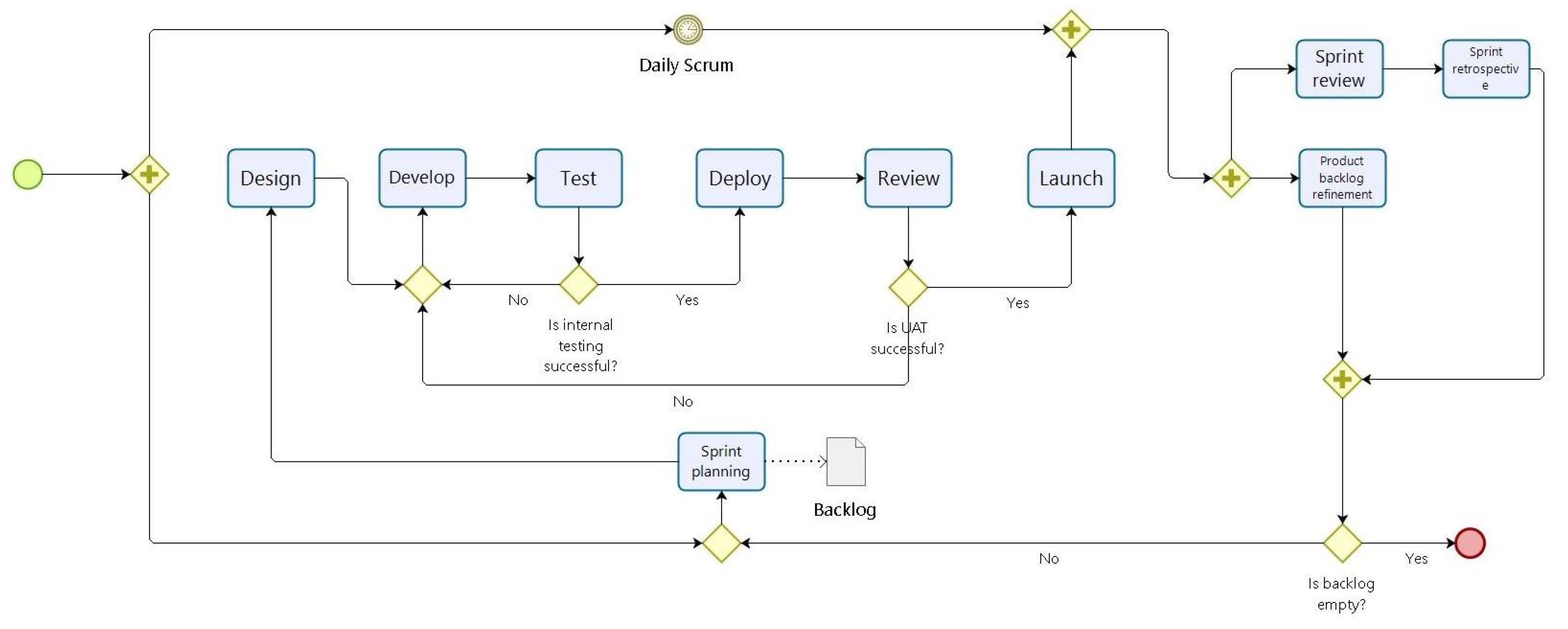
Based on the Agile idea presented in [39], an Agile SDP model is presented in Figure 1.

The Agile methodology is iterative, with specific “ceremonies” that must be repeated after every iteration [39]. The main iteration is a sprint, which has six main stages: design, develop, test, deploy, review, and launch. When all of these stages are complete, another iteration can be moved to. The main ceremonies for Agile SDP are as follows:

• Daily scrum—a short meeting that repeats every working day and usually takes up to 15 min. A daily scrum seeks to efficiently use delivery team time and resources for problem solving or sharing relevant information.
• Sprint planning—an activity that starts each sprint, where all stakeholders discuss which product backlog task will be included in the next sprint.
• Sprint review—an activity that takes in the previous sprint to share the accomplishments of the sprint with the delivery team.
• Sprint retrospective—the final activity in the sprint. During this phase, the entire delivery team should discuss the sprint’s successes and emphasize things that could be improved.
• Product backlog refinement—this activity takes place towards the completion of a sprint. Here, the backlog is reviewed and kept clean and ready for the next sprint.

4.2. Case-Handling for the SDP Model

Case-handling is a paradigm that enables flexible, knowledge-intensive BPs. It is heavily reliant on data [40,41] and mainly focuses on what can be done to achieve a business goal rather than using established process control structures describing what should be done during a workflow process. When it comes to case handling, the knowledge worker in charge of a certain case actively decides how the goal of that case will be met. In the case handling allocation system, workers are aware of the whole case at any time, which can be advantageously viewed as a single BP instance. This decreases processing time and eliminates errors because the knowledge worker is already aware of the situation and can address difficulties and handle them quicker than a colleague who is unfamiliar with it [22]. Case handling is the most suitable option to model dynamics and parallel activities because of its focus, flexibility, and adaptation to different types of BP.

Since an Agile SDP is a knowledge-intensive process and highly depends on data, which are presented in the form of SDP development characteristics, the case handling approach is suitable and can be used for the modeling and simulation of Agile SDP models. Moreover, the core features of case handling [41] are well suited to modeling an Agile SDP as they enable users to:

• avoid context tunneling—all information about a particular Agile SDP is separated from other SDPs and provided as a whole and separate piece;
• decide which activities are enabled based on the information available—the knowledge worker is responsible for BP execution;
• divide task distribution and authorization and accept roles other than the execute function;
• add or modify data after activities have been executed—whether dynamically or in parallel.

4.3. Requirements for the SDP

Based on previous work that has already described the requirements for SDP modeling [27], the following requirements are defined for the developed SDP CMMN model:

• The model should describe and show the dynamics of activities and tasks in a subject area.
• It should be possible to define and observe the context or the business environment of the SDP instance.
• Knowledge workers should be responsible for the sequence of activities and the method of how the goal of the SDP is reached.
• The focus should be placed on a single process instance rather than on a workflow.
• The parallel modeling of activities or the parallel assignment of activities to one resource in the same or separate cases should be supported.
• There should be the possibility to assign risks for activities.

These requirements were developed based on the main software development features.

4.4. Fuzzy Inference in the SDP Model

The SDP is a dynamic and knowledge-intensive BP because of HFs within process activities. As it is very difficult to predict how HFs influence one another in the implementation of an activity, we take them as fuzzy variables.

The influence of the HF on the SDP can be expressed as $HF\left(f_1,f_2,\dots ,f_n\right)$, where f_i denotes a particular attribute of a resource. In this research, we emphasize such resource attributes as motivation (f₁), experience (f₂), and availability (f₃).

Consequently, a linguistic variable of HF consists of linguistic attributes f_i—such as motivation (f₁), experience (f₂), and availability (f₃)—whose value set T can, in turn, be divided into meaningful crisp intervals, and whose linguistic meaning denotes the human linguistic attribute level as Excellent (5), Good (4), Moderate (3), Low (2), or None (1).

We chose these HF variables because it is already established that motivation, experience, and availability can make a difference in the performance of any human-related activities. For example, employee motivation is considered a force that drives employees towards achieving specific goals and objectives [42,43]. In [42], the authors observed that a significant and positive relationship exists between employee motivation and employee performance. Employee experience level turns human resources management in an organization into a more strategic process that engages the employee through meaning and providing value [44]. Availability is the parameter that shows how much time a resource can be used for task execution. It is very important to include the possibilities of HFs in BP simulation in order to achieve more precise values of task execution time and to see the impact of deviation from the estimated time.

In this paper, HF motivation (f₁), experience (f₂), and availability (f₃) are not measured, as this is not the main aim of this study. However, since it is important to estimate these factors, their values are randomly generated, and the total HF is inferred using ANFIS.

ANFIS is an FIS implemented within the framework of adaptive neural networks [45]. It is based on a set of fuzzy IF-THEN rules (e.g., (1)), with the MFs appropriate to generate specified input-output pairs:

$$R_i:if \left(x_1 is A_1^{\left(i\right)}\right)\dots and\dots \left(x_n is A_n^{\left(i\right)}\right) then f_i=a_i^T ·x+b_i ,$$

(1)

where $x ϵ {ℝ}^n$ is a vector of inputs in the presumption characterized by an appropriate MF, and $a_i,b_i$ are the coefficients of linear Takagi–Sugeno consequents. Training ANFIS means determining parameters belonging to the components of the premise (i.e., input parameters) and the consequences (i.e., output) of using an optimization algorithm [45].

The principal schema of ANFIS consists of five layers, as follows [45]:

Layer 1. Fuzzification: inputs ((x₁, x₂), $n=2$) are fuzzified using trapezoidal MFs whose parameters—${\mathrm{c}}_1$, ${\mathrm{c}}_2$, ${\mathrm{c}}_3$, ${\mathrm{c}}_4$—are both adaptive and adapted during the learning. As the values of the parameters change, the MF of the linguistic term $A_n^{\left(i\right)}$ also changes [45].

Layer 2. Evaluation of the rule strength: each node provides the rule strength, $w_i$ (Equation (2)) [45]:

$$w_i=\prod {\mu }_i\left(x\right),$$

(2)

Layer 3. Normalization: the strengths of all rules, $w_i$, are normalized (${\overline{w}}_i$) (Equation (3)) [45]:

$${\overline{w}}_i=\frac{w_i}{{{\displaystyle \sum }}_{\mathrm{i}}{w}_i},$$

(3)

Layer 4. Application of the rule ($R_i$) to obtain the output $f_i$ [45].

Layer 5. Computation of the global model response (f) is given in Equation (4) [45]:

$$f={{\displaystyle \sum }}_i{\overline{w}}_i{f}_i,$$

(4)

After training is complete, ANFIS performance is determined by various statistical tests [46]. This study used the following statistical tests: coefficient of determination (R²), mean squared error (MSE), and root mean squared error (RMSE).

The coefficient of determination (R²) [46] is used to analyze how differences in one variable can be explained by differences in another variable (see Equation (5)). It ranges in the interval [0, 1].

$$R^2=1-\frac{S{S}_{res}}{S{S}_{tot}}, \mathrm{where} S{S}_{tot}={{\displaystyle \sum }}_i{\left({f_{train}}_i-\overline{f_{train}}\right)}^2 \mathrm{and} S{S}_{res}={{\displaystyle \sum }}_i{\left({f_{train}}_i-f_i\right)}^2,$$

(5)

where $S{S}_{res}$ denotes the sum of the squares of residuals, and $S{S}_{tot}$ the total sum of squares.

The mean squared error (MSE) [41] (Equation (6)) is used to measure the average of the squares of errors between the output f and the training $f_{train}$ values.

$$MSE=1/n{{\displaystyle \sum }}_{i=1}^n{\left(f_i-{f_{train}}_i\right)}^2,$$

(6)

The predicted result is more precise when the value of MSE is closer to zero.

The root mean squared error (RMSE) is a metric commonly used for comparing values predicted by a model or estimating in relation to values actually observed. RMSE is defined as the square root of the average squared distance between the actual score and the predicted score [46] (see Equation (7) [47]).

$$RMSE=\sqrt{\frac{{{\displaystyle \sum }}_i{\left(f_i-{f_{train}}_i\right)}^2}{n}},$$

(7)

RMSE is always non-negative and has a value of zero when the data fit perfectly. A lower RMSE is often preferable to a higher one [47].

The sum of squares is a statistical measure of deviation from the mean. The sum of squares due to error (SSE) measures the total deviation of the response values from the fit to the response values [48] (see Equation (8) [47]).

$$SSE={{\displaystyle \sum }}_{i=1}^n{\left(f_i-{f_{train}}_i\right)}^2,$$

(8)

The fit will be better for prediction if the SSE value is closer to 0, which means that the prediction model has a reduced random error component [47].

4.5. Simulation of the SDP Model

Agent-based modeling and simulations are the most suited for simulating dynamic processes with human actors. This method of simulation provides an opportunity to simulate human behavior, its changes according to psychological aspects, the order of work performance, and changing conditions that can influence the outcome of the BP. Agent-based modeling and simulation can also be called multi-agent modeling and simulation or multi-agent-based modeling and simulation (ABMS). In ABMS, active components or decision makers are conceptualized as agents, whose activities are simulated using the agent-based simulation (ABS) paradigm according to agent-based modeling (ABM). The ABS model system is composed of agents that follow a sequence of predefined rules to achieve goals that interact with the environment. The main idea behind ABMS is to represent a phenomenon that can be generated by a multi-agent system. This agent-based modeling and simulation is suitable for systems that address social phenomena in various disciplines, such as traffic detection. The creation of an agent-based model involves three main stages:

• The identification and creation of agents.
• The identification of the relationships between agents and their relationships with the environment.
• The identification of the environment in which the simulation will take place [49].

To simulate the SDP and depict its dynamic execution using the CMMN model, the agent-based simulation method is the most appropriate, as it can properly illustrate the behavior of case executors and SDP roles at different stages of SDP implementation.

4.6. The Proposed Approach

The SDP CMMN model is developed according to the following aspects:

• CMMN requirements and notation.
• Agile methodology.

The developed SDP model has input parameters from task consistency and dependency analysis, role analysis, and task time estimates. A business case simulation tool is a tool that simulates a real software development case with selected input data. The simulation tool consists of three separate modules: simulation scenario specification, simulation scenario execution, and report generation. In the report generation module, simulation scenario configurations and historical data may be useful in the future to evaluate performance or progress based on specific data, simulation execution data, and report templates. The input data of the business case simulator tool are formed from the specifications of the tasks and resources. The more accurate and detailed these specifications are, the more accurate the input data will be and the more consistent the simulation results will be with the model. The output of this is a case execution report, generated according to report templates and to the needs of the business or SDP team.

Using the proposed CMMN model SDP, software development modeling and simulation is performed at the initial state of SDP execution, when the user’s needs are defined. These needs are used to define the initial variables for the proposed CMMN model input. After the successful verification of all input data, the simulation can begin. The accuracy of the simulation results depends on the level of detail and accuracy of the initial data. The obtained results show the potential risks to the SDP, such as possible delays, working outages, places where resources are not fully utilized, and so on. Thus, the analysis of the simulation results is important as it identifies problems and possible future challenges of the SDP. Based on the analysis of the obtained results, a new assigned resources plan can be developed before re-simulation. Plan refinement and simulation are performed as many times as possible until a suitable plan meets the user’s needs.

If necessary, SDP simulation can be done during the execution of the SDP. In most cases, this is necessary when unpredictable changes occur, such as changes to the user’s needs.

4.7. Dataset in the Research Method

To execute experiments, there is a need to describe the dataset. For the simulation model dataset, actual roles and tasks for SDP are listed. Every task has been assigned its own estimated task execution time. All listed roles are described by parameters of HF. The complete dataset for the simulation includes:

• List of roles.
• Estimated task execution time.
• Role—task mapping table.

5. A Case Study

The proposed CMMN model for SDP simulation was implemented in the prototype using the Python programming language (https://www.python.org/, accessed on 1 June 2022) with the Mesa plugin (https://mesa.readthedocs.io/en/stable/, accessed on 1 June 2022) (see Figure 2). Mesa is used to simulate the developed CMMN model. For the implementation of the proposed CMMN model, Flowable (https://flowable.com/, accessed on 1 June 2022) was used. Requests are sent from Mesa to the Flowable REST API to retrieve input data, which defines a sequence of SDP activities, their duration, and constraints in .csv format. The output data are then saved in the form of an electronic spreadsheet tool (.csv) and are unique during each simulation. The choice of the Python language was based on specific advantages. For example, as a dynamic programming language, Python is widely used in many fields. From the perspective of developers, various language features affect the programming experience. Researchers can then affect the difficulty of developing tasks, such as bug finding and compilation [50].

5.1. Experiment Data

Firstly, we detailed which roles are the most important and necessary for an Agile SDP. These roles are: IT analyst (analyst in input file); product owner (po in input file); scrum master (sm in input file); quality assurance specialist (tester in input file); and developer (developer in input file). An example of the input data is presented in

Table 1. Input data example.

Name	Order	Estimation	Role
create product backlog	1	2	po
sprint planning	1	2	sm
design	1	4	analyst
develop	1	10	developer
test	1	3	tester
deploy	1	2	developer
review	1	1	developer
daily scrum	1	1	developer
launch sprint	1	1	developer
sprint review	1	2	sm
sprint retrospective	1	2	sm

. The order of tasks in an SDP must be listed so that it is clear which task has a higher priority and must be performed at an earlier stage of the process. The estimation column represents how much agent resources are required in order to complete the task. The role column assigned to each task means that this task can only be performed by this role.

The role-agent mapping table is also an input (see

Table 2. An example role-agent mapping and agent specifying table.

Name	Role	Motivation	Experience	Availability
Agent 1	analyst	1	4	3
Agent 2	po	3	5	4
Agent 3	tester	1	2	4
Agent 4	sm	1	4	4
Agent 5	developer	2	4	1

). The second input file provides a list of agents and their number. Each agent has their own role, which means that this agent can do only those tasks assigned to their role (from Table 1). In this list, it is also necessary to specify all agents’ HFs and provide a value for every factor from 1 to 5 (Excellent (5), Good (4), Moderate (3), Low (2), None (1)).

For the experiment in this study, we used randomly generated input data based on a theoretical description of an SDP and practical experiences. The execution of the entire SDP in the company could involve many different roles, between which tasks are divided at different stages. Because of the case model, that shows which tasks and stages can be started dynamically and which can be started consistently, the distribution of tasks between roles can allow for maximum optimization, execution time, and choice of resources regarding the SDP. The main SDP roles are scrum master, product owner, analyst, developer, and tester. All SDP tasks and roles are mapped between them to assign all SDP activities to the appropriate role.

During the experiment, the input data had to be examined and systematized. To simulate the CMMN model of the SDP, it is important to identify the execution time for each task. It is impossible to assess precisely and in detail the tasks of each SDP implementation activity as they strongly depend on the subject area in which the SDP takes place. Each subject has its own specifics which are relevant only to specific aspects, and this has a direct effect on the time it takes to execute a task.

All of the agents involved in the simulation are brought together and assigned roles, according to which SDP tasks are then assigned. It is necessary to have all roles in order to successfully complete a process simulation, as not performing a particular task does not allow the whole simulation case to be completed.

The simulation also includes the priorities for each task, the estimated execution times, and the role of the agent or agents that will be able to perform the task. Agents with different roles can also perform the same tasks depending on their experience or competence. According to the agent, it is also possible to reduce or increase the scheduled execution time of the task. This was changed and updated during the simulation, but the structure was kept the same. The task and role data were described in the input data document in the same way as it is saved in the model builder itself: by ID value.

5.2. Modeling the SDP with CMMN

The CMMN model for the simulation of the software development process was developed in order to depict all relevant tasks and distribute them according to the stages of the process.

As we take the Agile methodology as the basis for SDP simulation, we divide the SDP into two main stages: the sprint itself, and activities after the sprint. In Figure 3 can be seen that the process can be started by creating a product backlog and placing the most important changes into the subsequent sprint. The sprint is commenced after successful planning, when the sprint stage is activated. This stage involves six main tasks: design, develop, test, deploy, review, and daily scrum. The daily scrum is the only task that is independent of other tasks in this stage. After the sprint stage, the process is divided into two milestones in parallel: “Sprint is done”, and the activation of the other stage, “After sprint activities”.

It is possible to terminate the case in the following scenarios:

• The deadline of the SDP passes and all tasks in the case have not yet been completed.
• The backlog of product development becomes empty.

In this CMMN SDP model, there are some tasks that are based on the HF. The duration and quality of the performance of these tasks can be dynamic and can depend on HF resources. All tasks are assigned to particular agents with the competence required for task execution.

5.3. ANFIS in SDP Simulation

In this step, we loaded a HF dataset into ANFIS and performed FIM optimization. For this stage, we generated a dataset with all possible combinations of HF parameter values. We took possible values for three HF parameters and assigned possible deviations from the estimated task execution time value. These possible deviations are values that show how the initial parameter values (in columns 1–3) could vary because of HF influence. For example: if employee motivation, experience, and availability are low, the possible deviation value from the estimated task execution time is 1. In

Table 3. Snapshot of input values.

Motivation	Experience	Availability	Possible Deviation
1	1	1	1
2	1	1	1.3333
3	1	1	1.6667
4	1	1	2
5	1	1	2.3333
1	2	1	1.3333
2	2	1	1.6667
3	2	1	2
4	2	1	2.3333
5	2	1	2.6667
1	3	1	1.6667
2	3	1	2

, a snapshot of input values is presented.

Table 4. Possible deviation explanation according to numeric value.

Numeric Value	Possible Deviation Value	Explanation
[1; 2)	Very high	30% above estimated time
[2; 3)	High	20% above estimated time
[3; 4)	Moderate	10% above estimated time
[4; 5)	Low	No deviation from estimated
5	None	10% below estimated time

presents experts’ opinions, in numbers, on the possible deviations according to the HF values from Table 3. These experts were selected from various role groups as follows: four project managers (ex₁–ex₄) and four specialists—developers, analysts, and quality assurance specialists (ex₅–ex₈).

Experts were interviewed to determine the importance of the attributes presented, after which findings were processed [51]. The correctness of expert answers was determined, and the results were acceptable.

For the prediction of possible deviations in HF values, we used all possible combinations for the values of the three described HF factors (motivation, experience, and availability). All possible values were contained in 125 rows, so we divided the dataset and took 70% of the data for training, 15% for testing, and 15% for checking.

ANFIS hyper-parameters for optimization with crisp data are shown in

Table 5. ANFIS hyper-parameters.

Hyper-Parameters	Description/Value
Fuzzy structure/FIS training data	Sugeno/genfis1
Generation of FIS object	grid partition on the data
MF type (Input/Output)	Trimf/linear
Number of variables (inputs/outputs)	3/1
Number of terms (Input1/Input2/Input3)	3/9
Optimization method	backpropagation
Maximum number of training epochs	200
Initial step size	0.001
AndMethod/OrMethod/ImpMethod/ AggMethod/DefuzzMethod	prod/probor/prod/sum/wtaver
Data for training/data for testing/data for checking	70/15/15
Number of rules	27

.

The principal schema of fuzzy inference with ANFIS is presented in Figure 4.

Fuzzification and MFs are obtained from the input data in Layer 1 (Motivation, Experience, and Availability). Each MF is shown as an adaptable node, as can be seen in Figure 4. By compiling all feasible MF pair combinations, the fuzzy rules are created, and Layer 2 of the ANFIS network is formed. As a result, we now have 27 pairs of three inputs. The rule strengths are provided as non-adaptive nodes in Layer 3 after being adjusted. Moreover, in Layer 4, defuzzification is performed, and fuzzy rules are applied by adopting each node. The summation layer, or Layer 5, contains a single, fixed, non-adaptive output of the whole ANFIS network that has been obtained. The Fuzzy Inference Controller’s 27 fuzzy rules and MF parameters are then put into ANFIS. As a result, those MF parameters and fuzzy rules from FIS are optimized in ANFIS using objective, precise data. Following this optimization, the fuzzy rules and optimized parameters are retransmitted to the Fuzzy Inference Controller. The Fuzzy Inference Controller also performs inference using the optimized MF parameters and fuzzy rules.

According to the above process, following optimization, the value of the HF in the SDP can vary and may fall into a different predetermined linguistic term interval. As an illustration, the possibility of deviation is moderate prior to optimization and increases after optimization. The resulting surface of the optimized HF in the SDP is presented in Figure 5.

In this study, FIS used three input parameters with three fuzzy sets for each input to create a complete rule set of 27 rules for building the ANFIS model. It is important to note that increasing the partition size of the input space exponentially increases the number of influencing rules, greatly improving the speed of system learning and application.

Some examples of the fuzzy rules are as follows:

• IF (hf1 is None) AND (hf2 is None) AND (h3 is None) THEN (PD (Note: Possible deviation) is Very High);
• IF (hf1 is None) AND (hf2 is Good) AND (h3 is Moderate) THEN (PD* is High);
• IF (hf1 is Moderate) AND (hf2 is Excellent) AND (h3 is Good) THEN (PD* is Low);
• IF (hf1 is None) AND (hf2 is Low) AND (h3 is Good) THEN (PD* is High);
• IF (hf1 is None) AND (hf2 is Good) AND (h3 is Good) THEN (PD* is Moderate).

The influence of HF in SDP prediction after optimization employing ANFIS is presented in Figure 6.

5.4. ANFIS Validation

The trained ANFIS was checked for validity using 15% of the data, employing the previously described statistical tests (R, MSE, RMSE). Experiment results values are in

Table 6. Statistical test values.

Statistical Tests	Experiment Results
SSE	4.839506
SST	80
SSR	60
R2	0.75
RMSE	0.19687136
MSE	0.03871608

.

As can be observed, the implemented SDP prediction systems perform sufficiently accurately and can be used for predicting the execution time of SDP tasks.

Additionally, a manual validity check of the trained ANFIS was performed with Simulink, using random initial data (see Figure 7).

A snapshot of the obtained results is presented in

Table 7. An example of the results with the proposed approach (possible deviations in numerical value).

HF1	HF2	HF3	Output (Possible Deviation)
2	4	2	2.667
1	4	5	3.333
5	3	2	3.333
1	2	3	2
2	2	2	2
5	4	2	3.667
4	3	3	3.333
1	2	1	1.333
4	2	5	3.667
1	1	2	1.333
2	4	2	2.667
1	4	5	3.333

. The obtained results correspond to ANFIS testing results, as presented in Figure 8.

The major challenge for the proposed approach and its implementation is the collection of reliable data and the ability to estimate every described resource. The use of ANFIS for HF impact prediction and calculation demonstrates the flexibility of the data transfer according to different HFs in the SDP context.

5.5. SDP Simulation Results

During each iteration, all agents were transitioned into what SDP tasks they can currently work on. If no active tasks were found for the respective agent during the iteration, a message is displayed, and the agent waits for the next iteration.

During the simulation, we can see the event log entries (Figure 3), which show the entries for each iteration. It is possible to monitor: how many and which tasks were found during the iteration of a particular agent, with the role assigned to them; which task was started; and the agents that did not find any active tasks during the iteration.

The results of the output data of the simulation are saved in electronic spreadsheet format and include: number of iterations; creation time; priority; task; agent; estimated time; and actual time. The amount of stored output data directly depends on the input data. The simulation output data show the number of iterations, which agent performed each specific task, when it was commenced, the estimated time for the task, and the actual time in which the task was performed.

Simulation results are exported in an output file in .csv format. We divided simulation results into two parts: simulation without HF prediction, and simulation with HF prediction.

Table 8. Simulation without HF results. Example of output file.

Create Time	Priority	Task	Agent	Estimated	Actual Time for Task Execution without HF	Actual Time for Task Execution with HF
2023-01-08 T19:19:05.374+02:00	1	create product backlog	Agent 2	2	1	2.0
2023-01-08 T19:19:06.849+02:00	1	sprint planning	Agent 4	2	1	2.4
2023-01-08 T19:19:12.159+02:00	1	review	Agent 5	1	1	1.2
2023-01-08 T19:19:12.158+02:00	1	design	Agent 1	4	1	4.8
2023-01-08 T19:19:17.834+02:00	1	develop	Agent 5	10	7	12.0
2023-01-08 T19:19:23.395+02:00	1	test	Agent 3	3	1	2.4
2023-01-08 T19:19:12.159+02:00	1	daily scrum	Agent 5	1	1	3.59
2023-01-08 T19:19:12.158+02:00	1	deploy	Agent 5	2	5	1.2
2023-01-08 T19:19:34.039+02:00	1	sprint retrospective	Agent 4	2	1	1.2
2023-01-08 T19:19:34.038+02:00	1	launch sprint	Agent 5	1	5	2.4
2023-01-08 T19:19:34.039+02:00	1	sprint review	Agent 4	2	2	2.4

presents the results of SDP simulation with and without the HF.

As a result (Table 8), we achieved more precise actual task execution times according to the described values with all three HF input variables.

A comparison of the obtained results is presented in Figure 9.

From these results, we can see how actual times for task execution can vary depending on the HF. For example, as can be seen in Figure 10, Agent 5 will take longer than expected to perform the development task because of their HFs. Conversely, the deployment task will be executed much more quickly, despite the fact that this is the same agent with the same HF values. These results show that the prediction and calculation of the HF helps to simulate the SDP in a more precise way and shows the actual time taken for tasks according to changes in the HF rather than varying randomly.

Figure 11 compares the minimum and maximum deviation of estimated task execution time when the simulation is performed without HF prediction and with HF prediction. It is visible that when task estimated time is small and takes 1–3 estimated units, the difference between possible actual time with the HF is much lower than without the HF. For example, the “Review” task is estimated to take 1 unit. The maximum possible value without the HF is 6, and the possible maximum value with the HF is 1.3. This means that possible deviations between the actual time are 4.7 units with this particular task, and it may exceed the estimated time by more than 3-fold. These results show that the inclusion of the HF in the SDP simulation model allows users to reduce possible maximum deviations between task execution times.

6. Discussion

In this paper, a fuzzy and case-based dynamic SDP modeling and simulation approach has been developed and simulated to validate its performance. The advantages and uniqueness of the proposed approach are as follows: (1) it allows dynamic and parallel SDP modeling and simulation by applying a case-handling approach; (2) an ANFIS-based model is established to predict the influence of the HFs on the SDP; and (3) the simulation is implemented through the CMMN model.

Based on the related works, the main uncertainties affecting the dynamism of BPs are the following: the behavior of process resources; changing conditions; and the sequence of tasks. First, the behavior of process resources mainly concerns the HFs, the competencies of resources, and psychological aspects. Therefore, we added an HF prediction method based on ANFIS to predict the effect of the HFs on the SDP more accurately. Second, changing conditions are related to the SDP context and application domain. As the SDP is dynamic, changing conditions can impact the specifics of each software product. Therefore, additional components for describing and managing a context and application domain are necessary for SDP simulation. Consequently, the changing conditions of the SDP are modeled by applying CMMN. Finally, the sequence of tasks is one of the uncertainties affecting the dynamism of BPs, as it can change depending on the scope of the SDP and the state of the software product. In summary, the proposed fuzzy and case-based dynamic SDP modeling and simulation approach has advantages and contributes to SDP modeling and simulation by considering the HFs, process dynamism, and changing contexts. All of these factors allow for SDP modeling and simulation that is more in line with reality.

In terms of design, the contribution of this research lies in successfully implementing and demonstrating the proposed fuzzy and case-based dynamic SDP modeling and simulation approach in a prototype and conducting experiments with it. Two types of experiment were conducted as follows: (1) without including the HF in SDP modeling and simulation and (2) with the inclusion of the HF in SDP modeling and simulation. Finally, the results of both experiments were compared using statistical tests and the minimum and maximum deviation of estimated task execution time.

The obtained results show that the inclusion of the HFs in SDP modeling and simulation may lead to different results in predicting the execution time of SDP tasks than we would achieve without the inclusion of the HFs. The most significant possible differences between the results of both experiments were obtained when the person is entirely unmotivated (i.e., the HF is low, in which case the SDP execution time deviation is the largest). Consequently, including the HFs in SDP modeling and simulation can lead to the more realistic prediction of SDP task execution time.

Another advantage of the proposed approach is that it can be adapted to different SDP methodologies by adjusting the proposed SDP CMMN model. Moreover, other HFs can be used for SDP modeling and simulation, such as by changing the composition of the HF itself and increasing or decreasing the sensitivity of the model to the HF by increasing or decreasing the number of linguistic terms.

This research also shows the suitability of ANFIS for HF prediction in the software product development area. The accuracy of the statistical tests (MSE = 0.196872, RMSE = 0.038716) obtained in this research shows the well-fitting predictions provided by the trained ANFIS model.

Limitations of the Current Approach and Future Works

This research has some limitations. The main drawback is that the simulation results are based on randomly generated HF data. It would be more precise if data were to be gathered from a real SDP. Moreover, this could ensure reliable verification of the proposed fuzzy and case-based dynamic SDP modeling and simulation approach. Consequently, the following future works are planned:

• Adapt other SDP methodologies with the proposed fuzzy and case-based dynamic SDP modeling and simulation approach.
• Gather data from real SDPs and prepare them for model verification.
• Extend experiments with different SDP data, such as by including new HF input parameters, changing or combining agent roles, and so on.
• Investigate the overfitting behavior of the model.

7. Conclusions

The analysis of related works on SDP modeling and simulation shows that most studies stem from a different point of view: costs, BPs, and IS interactions or software development management methodologies. In the analyzed models, the HF or other psychological aspects of human work are considered in software development management methodologies or BPs, IS interactions, or the cost of software product development. However, those models do not consider the influence of the HF on the SDP from an activity execution perspective. Within BP simulation, the activity execution perspective is important in determining the overall duration of the BP and possible outcomes. Consequently, including the HF in SDP modeling and simulation allows us to achieve a more realistic view of the execution of SDP activities in terms of their duration and possible outcomes.

The newly proposed fuzzy and case-based SDP modeling and simulation approach illustrates the software development execution process. Its first advantage is that the case-handling paradigm allows us to implement SDP dynamicity, since real SDPs are dynamic by their nature. The second advantage of the proposed approach is that it includes the HFs through its fuzzification in the simulation of SDP activities.

The proposed fuzzy and case-based SDP modeling and simulation approach was implemented in a prototype, and experiments were conducted in two ways: without HF prediction and with HF prediction. The results showed that the proposed approach of including HFs in the SDP simulation model allows us to achieve more precise actual task execution time and to predict possible SDP risks. Moreover, the experiments with ANFIS show that it is an accurate, suitable AI model for HF prediction, and its performance could be improved with more reliable data.

In summary, the proposed fuzzy and case-based SDP modeling and simulation approach is suitable for SDP execution prediction and the observation of possible risks.