Numerical Study on Cooling Performance of a Steam-Cooled Blade Based on Response Surface Method

Abstract

In order to investigate the cooling mechanism of the turbine blade and to enrich and supplement the experimental study of the blade, a numerical study of a steam-cooled blade with five cooling channels was carried out based on the response surface model. The surface cooling efficiency and dimensionless temperature distribution of the steam-cooled blade were obtained with different mainstream inlet temperature, outlet pressure, pressure ratio of inlet to outlet, temperature ratio and flow ratio of steam to mainstream by using the flow-solid coupling numerical method. The influence of the working parameters on the cooling performance of air-cooled blade and steam-cooled blade, including the average cooling efficiency, temperature non-uniformity, and average dimensionless temperature, was comparatively investigated; the correlation equation of the working parameters on the cooling performance of the steam-cooled blade was obtained. The results show that the influence of mainstream inlet temperature and outlet pressure on the cooling performance of the steam-cooled blade is not significant; the cooling efficiency of the steam-cooled blade increases by 5.92%, 7.35% and 26.51% respectively as the mainstream inlet to outlet pressure ratio, the temperature ratio and the flow ratio of steam to mainstream increase; the dimensionless temperature increases by 3.74% as the temperature ratio increases and decreases by 0.93% and 4.09% as mainstream inlet to outlet pressure ratio and flow ratio increase; the temperature non-uniformity decreases by 4.09% and 30.08% respectively, as the mainstream inlet to outlet pressure ratio and temperature ratio increase and increases by 37.99% as the flow ratio increases; the effect of working parameters on air-cooled blade and steam-cooled blade is the same, but the steam-cooled blade has 14.06–17.81% higher cooling efficiency, 18.47–29.01% higher temperature non-uniformity and 1.86–2.58% lower dimensionless temperature compared to the air-cooled blade under the same working parameters; the correlation equation obtained by fitting the response surface model has higher accuracy.

1. Introduction

Gas turbines are widely used in energy and defense fields such as power generation and mechanical drives, representing high-end core technology power equipment for national security and overall economic development [1]. With the increasing requirements for gas turbine performance in various industries, improving the performance of gas turbines has become an urgent problem at this stage, and one of the most effective methods is to increase the turbine rotor inlet temperature. The increasing turbine inlet temperature will pose a greater challenge to the life and safety of turbine blades [2]. Therefore, many experts and scholars have conducted comprehensive research on the cooling technology of high temperature turbine blades of advanced gas turbines [3,4,5].

At present, with the development of computational fluid dynamics and computer technology, the conjugate heat transfer numerical analysis method has been able to satisfy most of the heat transfer studies [6]. The blade experiments face difficulties such as expensive cost and difficult to guarantee the measurement accuracy, so the use of numerical methods to supplement the blade experiments and the investigation of the cooling mechanism will be one of the effective ways for the development of turbine blade cooling technology in the future. Many domestic and foreign experts and scholars have carried out numerical research on the cooling performance of the blade. Luo et al. [7] used the conjugate heat transfer method to predict the flow and heat transfer characteristics of NASA turbine blades under three operating conditions, and the results showed that the conjugate heat transfer method can be a feasible tool for turbine blade heat transfer analysis and cooling structure design. John et al. [8] showed that the calculation results of conjugate heat transfer analysis are more accurate than those of un-conjugate heat transfer because the conjugate heat transfer fully takes into account the effect of the distribution of solid surface temperature on the fluid thermal boundary layer. Prapamonthon et al. [9] investigated the cooling performance of turbine blade coated with thermal barrier using the conjugate heat transfer numerical method, and the results showed that the conjugate heat transfer numerical method can better predict the heat transfer coefficient of the blade surface and its internal temperature, etc. The results of Nowak et al. showed that the conjugate heat transfer numerical method predicted the blade temperature field very well [10]. Zhu et al. [11] used the conjugate heat transfer method to analyze the temperature and flow field distribution on the surface of turbine blades with thermal barrier coating for various turbulence models, and the results showed that the calculated results obtained by the conjugate heat transfer numerical method were in good agreement with the experimental results.

In recent years, machine learning methods have been gradually applied to cooling performance prediction of blades and cooling structure optimization of blades due to their excellent performance [12,13]. Abbasi et al. [14] numerically investigated the effects of injection angle, mass flow rate, diameter and position on the cooling efficiency of a gas turbine using the response surface method, and explored the sensitivity of the input parameters. Lakzian et al. [15] used response surface model to investigate the optimal width and location of air film holes in a turbine blade and analyzed the significance of the effects of eight design variables on blade performance. Mahdavi et al. [16] used the response surface method to determine the optimal location of a solar collector when a gas turbine system was at maximum net power, minimum CO₂ emissions, and maximum energy efficiency. Wang et al. [17] performed a comprehensive response analysis and sensitivity analysis of the cooling performance of a gas turbine based on deep learning data modelling, and the results showed that the model can provide accurate predictions and had a fast response time. In addition, in the cooling of turbine blades at high temperatures, steam has better advantages over air due to its better heat transfer properties [18,19]. Xing et al. [20] showed that better internal cooling performance of gas turbine blade can be obtained using steam cooling compared to air cooling. Najjar et al. [21] comparatively studied the cooling performance of blades under three cooling schemes (open-circuit steam, air and closed-circuit steam cooling) and showed that steam cooling has higher cooling efficiency compared to air cooling.

The above literature shows that response surface models can be used to predict the cooling performance of turbine blades well and that steam has better cooling efficiency than air, but very little literature has explored the effect of steam-cooled blade operating parameters on its cooling performance. In this paper, in order to refine the steam-cooled blade with five internal cooling channels, the blade cooling system was considered as a complex system, and the system can be precisely adjusted by changing the parameters such as mainstream inlet temperature, mainstream outlet pressure, mainstream inlet to outlet pressure ratio, temperature ratio and flow rate ratio of cold gas to mainstream. Secondly, most of the existing studies in the investigation of the cooling performance of the blade, most of the evaluation indexes used only cooling efficiency. While in this paper, in order to explore the cooling performance of the blade in more detail, adding the index that can visually reflect the cooling effect of the turbine blade—dimensionless temperature and the index that can reflect the cooling uniformity of the turbine blade—temperature non-uniformity.

Therefore, in this paper, based on the combination of experimental design and response surface modeling, the flow-solid conjugate heat transfer method was used to numerically study the steam-cooled high-temperature turbine blade, and the distribution rules of the cooling efficiency, dimensionless temperature and temperature non-uniformity of the steam-cooled blade under different inlet temperature of the mainstream, mainstream outlet pressure, pressure ratio of the mainstream inlet to outlet, temperature ratio and flow ratio of steam to mainstream were investigated. The difference of cooling performance between the steam-cooled blade and the air-cooled blade under different working parameters was investigated, and the empirical equation of the cooling performance of the steam-cooled blade was obtained by fitting the response surface model, based on which the significance of the effect of working parameters on the cooling performance of the steam-cooled blade was also investigated.

2. Numerical Methods

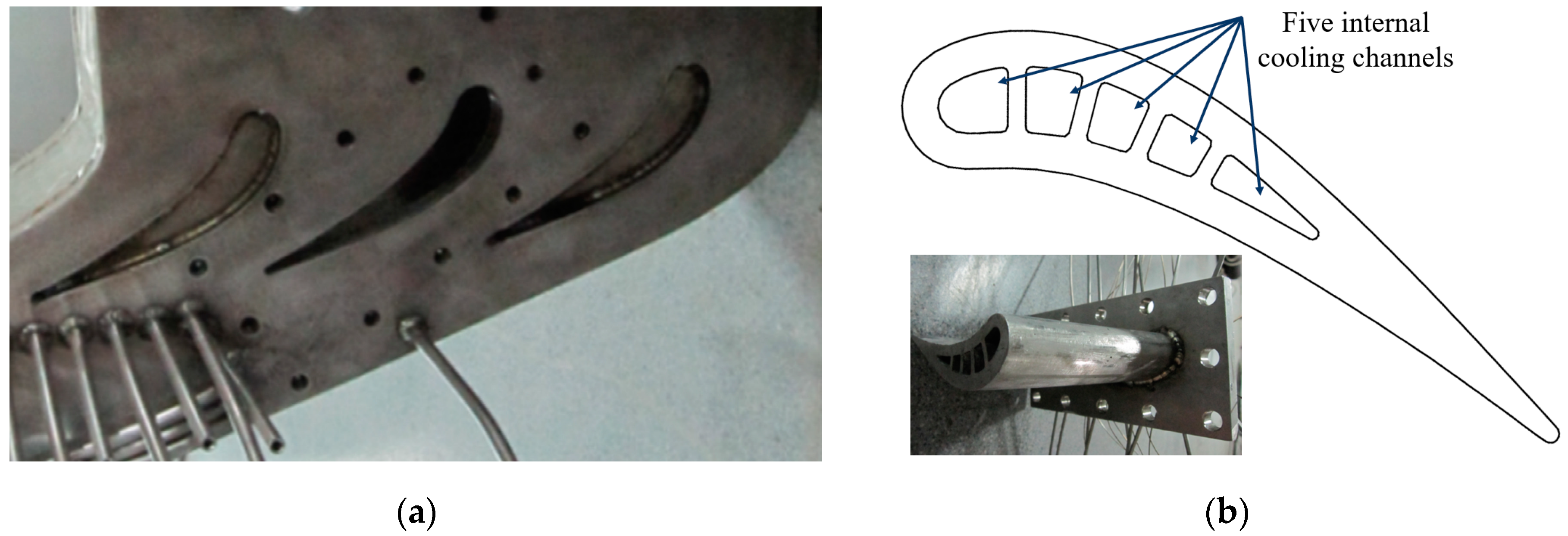
2.1. Subsection Physical Model

Figure 1 gives the experimental schematic diagram of the steam-cooled blade, the mainstream airflow is high temperature and pressure air, its flow rate can reach up to 2.3 kg/s, the temperature can be adjusted in the range of 323–823 K, and the maximum pressure can reach 0.7 MPa. Maximum flow rate of steam stream is 0.5 kg/s, the temperature distribution range is 373–523 K, the maximum pressure is 0.75 MPa. The main experimental equipment includes electric heater, steady flow section, steam generator, steam pipe, steam outlet and mainstream outlet. Therefore, the experimental system for steam-cooled vanes is mainly composed of the mainstream airflow and its heating device, steady flow section, cascade test section, steam airflow, data acquisition system, and exhaust system [22,23]. The mainstream provides a high-pressure mainstream airflow through the air compressor and electric heater, and the boiler provides the steam airflow. And when the cooling airflow is air, the airflow is provided by a small air compressor and a small electric heater. Figure 1 also shows how the test section is measured. The pressure measurement points and temperature measurement points are evenly arranged before and after the test section to obtain the inlet and outlet pressure and inlet temperature of the test section, and the temperature and pressure measurement points are evenly arranged in the blade mid-section and led out through the grooves on the blade surface for measurement. After calculation, it can be seen that the relative uncertainties of cooling efficiency, temperature non-uniformity and dimensionless temperature are 4.3%, 5.6% and 5.2%, respectively.

The cascade channel and the experimental blade of the steam-cooled blade are given in Figure 2, where Figure 2a shows the cascade channel and Figure 2b shows the experimental blade and its cooling structure. From Figure 2a, a solid blade without cooling structure is arranged on each side of the test blade in order to ensure the periodicity of flow in the cascade channel. In addition, half of the flow channels are extended on the outer side of the solid blade, forming a periodic cascade with three flow channels. Figure 2b gives the steam-cooled blade and its cooling structure, from the figure it can be seen that the leading edge of the steam-cooled blade to the trailing edge direction, five straight through cooling channels are distributed in an orderly manner, and the hydraulic diameters of the cooling channels are 0.0109 m, 0.0099 m, 0.0093 m, 0.0087 m, 0.0069 m in order. It is worth noting that the steam cooled blade is a straight blade made by stretching the middle section of the first-stage static blade of an F-class gas turbine, with a chord length of 123 mm and a height of 83 mm, made of 321 stainless steel 1Cr18Ni9Ti, which has a thermal conductivity of 16.3–22.2 W·m⁻¹·K⁻¹ and 321 stainless can function properly in the temperature range of 1023–1073 K.

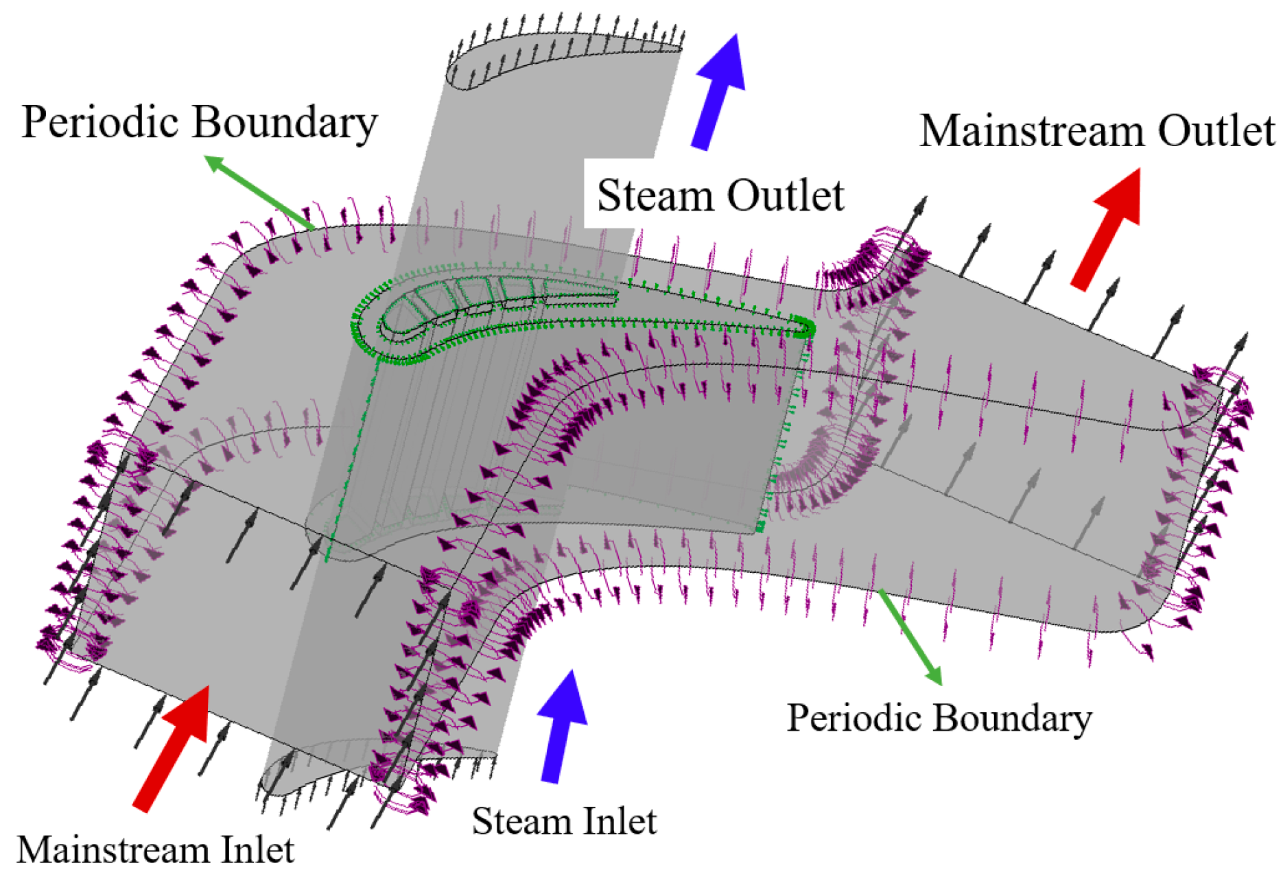
2.2. Numerical Methods

The numerical model of the steam cooled blade passage is shown in Figure 3. For the convenience of the study, the periodic passage with three flow channels in the test section is simplified to a single passage, and the flow channel on both sides of the blade in the numerical model is set to periodic boundary condition. For the accuracy of the numerical simulation, the inlet and outlet of the steam channel are extended by 100 mm each, which can make the numerical calculation better. The ANSYS CFX software (V18, ANSYS Inc., Pittsburgh, PA, USA) is used for the flow-solid conjugate heat transfer calculation. Since the flow-solid conjugate heat transfer method considers the influence brought by the solid heat conduction, it is widely used in the research of turbine blade cooling technology. The finite difference method based on finite elements is used to discretize the control equations and solve the three-dimensional compressible Reynolds time-averaged N-S equation, and the diffusion, source and convection terms in the equation are separated using a high-precision discrete format, and the residual targets for continuity, momentum and energy are set to 10⁻⁶.

The boundary conditions of the numerical calculation are basically the same as the experimental conditions, and the mainstream inlet is set as the total temperature and total pressure; the steam inlet is set as the static temperature and static pressure, and the turbulence level is 5%; the mainstream outlet is set as the average static pressure, and its value is the average value of the experimental obtained static pressure, and its value is allowed to vary within 5% of the average value; the steam outlet is set as the mass flow rate, and the magnitude is the experimental value. The fluid-solid contact surface is set as a flow-solid interface with the same temperature and heat flux distribution; the rest of the solid surface is set as the adiabatic wall surface. Figure 3 also presents the mainstream inlet, mainstream outlet, steam inlet, and steam outlet of the steam-cooled blade channel.

According to the research on turbine blade cooling performance by our research group [24,25], it is observed that the SST k-ω turbulence model has a high accuracy in the prediction of turbine blade cooling performance and is in the best agreement with the experimental data. To guarantee the accuracy and comparability of numerical simulation results, the SST k-ω turbulence model is also used in this paper for the numerical simulation of the steam-cooled blade channel. Menter et al. [26] proposed the SST k-ω model based on the k-ω model, using the k-ω model in the wall boundary layer and the k-ε model in the wall boundary layer, which can be used to improve the accuracy of the prediction of flow separation phenomena. The SST k-ω model equation is as follows:

$$\frac{\partial (\rho k)}{\partial t}+\frac{\partial (\rho k{u}_i)}{\partial x_i}=\frac{\partial }{\partial x_j}\left({\Gamma }_k\frac{\partial k}{\partial x_j}\right)+G_k+Y_k+S_k$$

(1)

$$\frac{\partial (\rho \omega )}{\partial t}+\frac{\partial (\rho \omega u_i)}{\partial x_i}=\frac{\partial }{\partial x_j}\left({\Gamma }_{\omega }\frac{\partial \omega }{\partial x_j}\right)+G_{\omega }+Y_{\omega }+S_{\omega }+D_{\omega }$$

(2)

The laws of conservation of mass, momentum and energy are used to solve the fluid domain, where the variables (u, v, w, T) all obey a universal conservation principle. By denoting the generic variables by ϕ, The control equation can be expressed in the following way:

$$\frac{\partial (\rho \varphi )}{\partial t}+div\left(\rho \overrightarrow{V}\varphi \right)=div\left({\Gamma }_{\varphi }grad\varphi \right)+S_{\varphi }$$

(3)

The blade material is made of 321 stainless steel, the density of which is 8030 kg·m⁻³ at 293 K and the specific heat capacity of which is 500 J·kg⁻¹·K⁻¹ at 273–373 K. The relationship between thermal conductivity and temperature of 321 stainless steel was fitted after reviewing the data [27]. It was linearly fitted into the material properties in the solver software, and the fitting equation is as follows:

$${\lambda }_{\mathrm{s}}=0.0148T+10.798$$

(4)

The cooling stream is steam, and the thermal physical parameters of the steam are calculated using IAPWS-IF97 data and interpolated from the local steam pressure and temperature. Dynamic viscosity and thermal conductivity of air fluids are solved using the Sutherland equation, and specific heat capacity is fitted to the equation by temperature. In addition, the air fluid is defined as an ideal fluid.

The flow-solid interfaces need to satisfy the conservation of variables such as temperature and heat flux, and the conservation equation is as follows:

$$q_{\mathrm{f}}=q_{\mathrm{s}},T_{\mathrm{f}}=T_{\mathrm{s}}$$

(5)

where q_f is the fluid wall heat flux/W·m⁻²; q_s is the solid wall heat flux/W·m⁻²; T_f is the fluid wall temperature/K; T_s is the solid wall temperature/K.

The solid domain requires only the solution of the heat conduction equation, which is expressed as follows:

$$\frac{\partial ({\rho }_s{c}_{s}T)}{\partial t}=\frac{\partial }{\partial x_j}\left({\lambda }_s\frac{\partial T}{\partial x_j}\right)$$

(6)

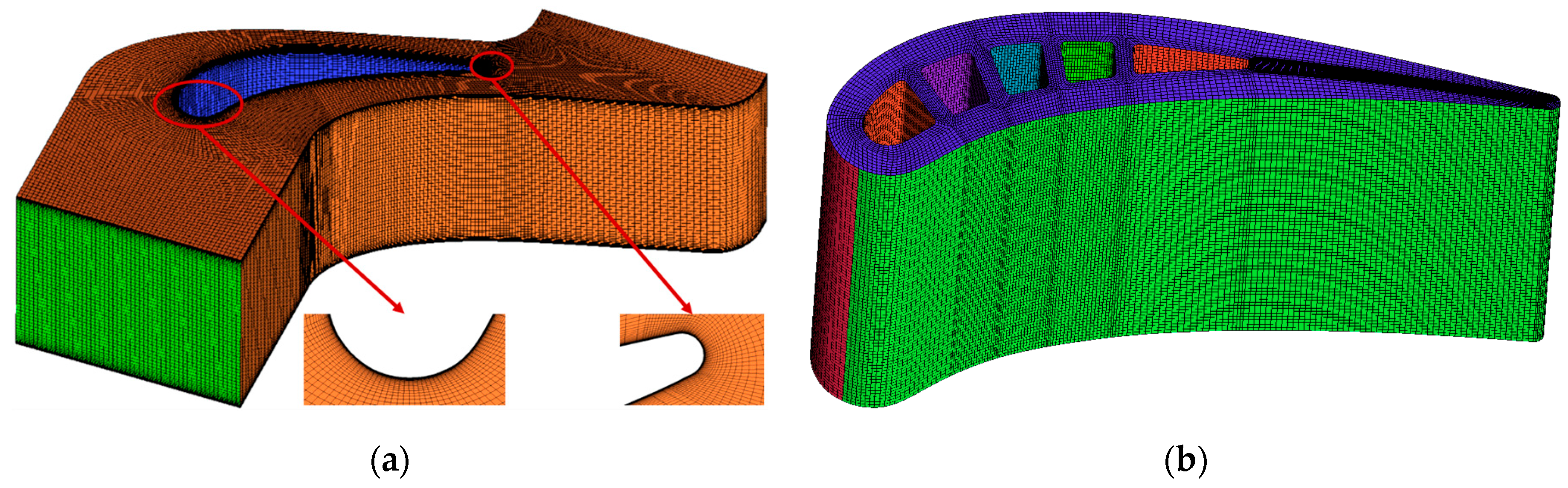
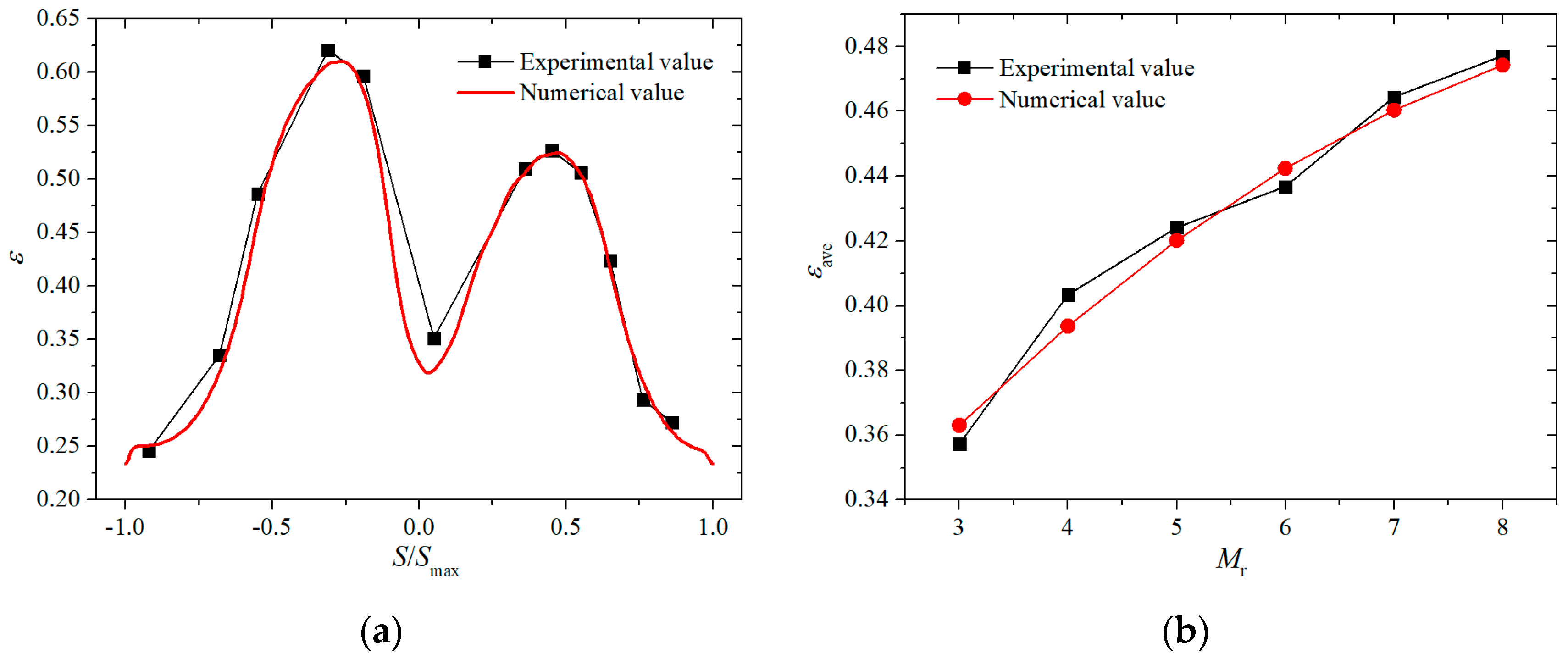
2.3. Numerical Verification

Figure 4 shows the mesh model of the steam cooled blade channel. As shown in Figure 4, both the fluid and solid domain meshes of the steam cooled blade channel are divided using structured meshing. Among them, Figure 4a is the fluid domain mesh of the cascade channel and neither is given because the meshes of the steam flow channel of the steam cooled blade and its inlet and outlet steady flow sections are simpler. To match the SST k-ω turbulence model, the mesh of the near-wall region of the fluid domain is refined, and the grid size of the first layer of the near-wall surface is set to 0.001 mm, the mesh growth ratio is 1.2, and the maximum grid size is 1.5 mm. Figure 4b shows the solid domain mesh of the steam cooled blade, and since the solid domain mesh does not need to be encoded, the minimum grid size is set to 0.5 mm. In addition, the mesh nodes at the intersection of the solid and fluid domains are matched to reduce the information transfer error at the fluid-solid interface.

To ensure the economic viability and reliability of the method of numerical simulation, mesh independence verification was conducted on the mesh of steam-cooled blade channel. A total of five sets of meshes were divided, and

Table 1. Mesh independence verification.

Fluid Domain Mesh	Solid Domain Mesh	Total Mesh Number	εave	ηave
1,098,756	118,740	1,217,496	0.355	0.799
1,617,840	209,874	1,827,714	0.384	0.812
2,014,780	319,871	2,334,651	0.411	0.834
2,478,210	422,968	2,901,178	0.431	0.849
3,047,180	512,950	3,560,130	0.433	0.853

shows the average cooling efficiency and average dimensionless temperature of the steam-cooled blade when the total number of meshes is 1.22, 1.83, 2.33, 2.9, and 3.6 million, respectively. From Table 1, It is clear that the average cooling efficiency and the average dimensionless temperature of the steam-cooled blade surface increase as the mesh number increases, in which the fluid domain mesh increases by about 500,000 each time and the solid domain mesh increases by about 100,000 each time. When the total number of meshes is increased from 2.9 million to 3.6 million, the differences of the average cooling efficiency and the average dimensionless temperature of the steam-cooled blade surface are less than 1%, which means that the mesh meets the requirements of mesh independence.

The experimental and numerically calculated values of the local cooling efficiency distribution and the average cooling efficiency on the surface of the steam cooled blade are given in Figure 5 for comparison. Figure 5a shows the local cooling efficiency distribution of the steam-cooled blade surface when the mainstream inlet temperature is 695 K, the mainstream outlet pressure is 140 kPa, mainstream inlet to outlet pressure ratio is 1.4, temperature ratio of steam to mainstream is 0.65, and the flow ratio of steam to mainstream multiplied by 100 is 5.5. As can be seen from Figure 5a, the distribution of the local cooling efficiency of the steam-cooled blade obtained from the numerical calculation and the experiment is in good agreement, and the trend of the two curves is basically the same, with a maximum deviation of 4.6%. Figure 5b shows the comparison between the experimental and numerical calculated values of the average cooling efficiency of the steam-cooled blade when the flow ratio of steam to mainstream multiplied 100 (M_r) increases from 3 to 8, with the remaining working parameters kept constant. From Figure 5b, it can be seen that the change trend of the average cooling efficiency of steam-cooled blade obtained from numerical calculation and experiment is basically the same, that is, the average cooling efficiency increases with the increase of M_r. At the same time, the average cooling efficiency of the numerically calculated blade is close to the experimental value. The maximum error appears when M_r is 4, the error is about 7.4%, and the average error is 4.9%. In addition, the literature [28] studied the blade structure is similar to this paper, its research results show that in k-ω, SSG, k-ω and SST k-ω turbulence models, the SST k-ω turbulence model can better predict the performance of the blade cooling, therefore, this paper also selected the SST turbulence model. Combined with the numerical verification of Figure 5 can be known that the SST k-ω turbulence model can accurately simulate the cooling performance of steam-cooled blade channel. Furthermore, the temperature distribution structure of the blade surface in the literature [28] was compared with the study in this paper, and the results showed that the distribution structure of both is quite similar. In summary, the numerical method of this paper concerning the cooling performance of steam-cooled blade channel is reliable.

2.4. Data Reduction

The cooling efficiency formula of the blade is as follows:

$$\epsilon =\frac{T_{\mathrm{gi}}-T_{\mathrm{w}}}{T_{\mathrm{gi}}-T_{\mathrm{ci}}}$$

(7)

where T_gi is the inlet temperature of mainstream/K; T_w is the temperature of blade surface/K; T_ci is the inlet temperature of steam flow/K.

The average cooling efficiency formula of the blade is as follows:

$${\epsilon }_{\mathrm{ave}}={\displaystyle \underset{A}{\int }\epsilon \mathrm{d}A}/A$$

(8)

where A is the surface area of the blade.

The dimensionless temperature formula of the blade surface is as follows:

$$\eta =T_{\mathrm{w}}/T_{\mathrm{gi}}$$

(9)

The average temperature of the blade is as follows:

$$T_{\mathrm{wave}}={\displaystyle \underset{A}{\int }{T}_{\mathrm{w}}\mathrm{d}A}/A$$

(10)

The average dimensionless temperature formula of the blade is as follows:

$${\eta }_{\mathrm{ave}}={\displaystyle \underset{A}{\int }\eta \mathrm{d}A}/A$$

(11)

The parameter to measure the temperature gradient of the blade is the temperature non-uniformity. The higher the temperature non-uniformity is, the more uneven the temperature distribution on the blade surface is. The formula is as follows [29]:

$$\zeta =\sqrt{{\displaystyle \underset{A}{\int }{(T_{\mathrm{w}}-T_{\mathrm{wave}})}^2\mathrm{d}A}/A}/T_{\mathrm{wave}}$$

(12)

Variation range of the working parameters for the steam-cooled blade is shown in

Table 2. Variation range of working parameters.

Working Parameters	Variation Range
Mainstream inlet temperature Tgi/K	680 to 710
Mainstream outlet pressure pgo/kPa	120 to 160
Mainstream inlet to outlet pressure ratio pr	0.6 to 0.7
Temperature ratio of steam to mainstream Tr	1.3 to 1.5
Flow ratio of steam to mainstream multiplied by 100 Mr	3 to 8

. It can be seen from the table that the working parameters include mainstream inlet temperature T_gi, mainstream outlet pressure of the p_go, mainstream inlet to outlet pressure ratio p_r, temperature ratio of steam to mainstream T_r, and flow ratio of steam to mainstream multiplied by 100 M_r. The variation range is 680–710 K, 120–160 kPa, 0.6–0.7, 1.3–1.5, 3–8 respectively.

3. Effect of Working Parameters on the Cooling Performance of the Blade

The temperature distribution and surface streamline distribution of the steam–cooled blade when the working parameters are both at the median value are given in 3D form in Figure 6 and Figure 7, respectively. As can be seen from Figure 6, the temperature at the tip of the steam–cooled blade is lower compared to the root. The steam–cooled blade mid-chord area has a lower temperature distribution compared to the leading and trailing edges of the blade. The temperature distribution of the leading edge of the steam–cooled blade is 580–630 K and the temperature distribution of the mid-chord area of the tip of the steam–cooled blade is the lowest, at 530–560 K. The trailing edge of the steam–cooled blade has the highest temperature distribution, at 630–650 K. In general, the temperature distribution of the pressure surface of the steam–cooled blade is lower than that of the suction surface. From Figure 7, it can be seen that the surface flow distribution of the pressure surface of the steam–cooled blade is more uniform, and the airflow velocity will gradually increase from the leading edge to the trailing edge of the blade. The surface flow line of the steam–cooled blade suction surface shows a tendency to gather in the trailing edge region of the blade, and the flow velocity of the airflow is larger at the location of the leading edge. In addition, the main purpose of this section is to study the influence of the working parameters on the cooling performance of the steam–cooled blade, and the subsequent for the convenience of the display, the cooling performance of the blade in 3D form is converted to 2D form, as detailed in Figure 8, Figure 9, Figure 10, Figure 11, Figure 12, Figure 13, Figure 14, Figure 15, Figure 16 and Figure 17.

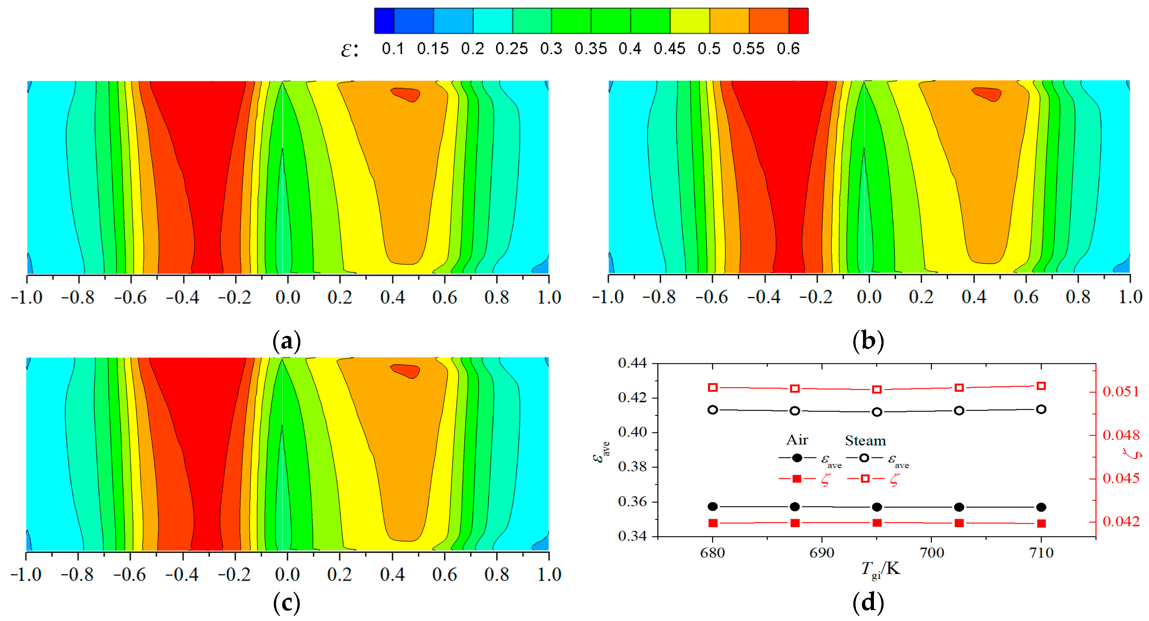
3.1. Influence of Mainstream Inlet Temperature

Figure 8 gives the influence law of the mainstream inlet temperature on the cooling efficiency of the steam cooled blade. In the figure, the horizontal coordinates −1–1 are the relative axial chord length of the steam cooled blade, −1–0 means the pressure surface of the blade, and 0–1 means the suction surface of the blade. When studying the effect of single working parameters on the cooling efficiency of steam cooled blade, the rest of the working parameters are in the medium value, such as studying the effect of the mainstream inlet temperature, the mainstream outlet pressure is 140 kPa, the mainstream inlet to outlet pressure ratio is 1.4, the temperature ratio of steam to mainstream is 0.65, the flow ratio of steam to mainstream multiplied by 100 is 5.5, the same below. From Figure 8a–c, it can be seen that the cooling efficiency of the steam cooled blade tip position is higher than that of the blade root position, which is because the steam flows into the blade from the blade tip and out from the blade root. The leading edge of the blade is directly impacted by the high temperature of the incoming flow, so it has a poor cooling effect, and the cooling efficiency is in the range of 0.25–0.35. The highest cooling efficiency region is in the mid-chord region of the tip of the steam-cooled blade, and the cooling efficiency can reach about 0.65. The tip and root positions of the trailing edge of the steam-cooled blade have the worst cooling effect, and the cooling efficiency is in the range of 0.15–0.2. Overall, the cooling effect of the pressure surface of the steam-cooled blade is better than that of the suction surface, which is probably due to the fact that the flow velocity of the suction surface is higher than that of the pressure surface and there is a reverse pressure gradient on the suction surface of the blade, so that the heat of the mainstream can be transferred to the surface of the blade more easily. In addition, from Figure 8a–c, it can be shown that the cooling efficiency distribution on the surface of the steam-cooled blade hardly changes when the mainstream inlet temperature is changed. This also indicates that the influence of the mainstream inlet temperature on the temperature nonuniformity of the steam cooled blade is also not significant. As can be shown in Figure 8d, the influence of mainstream inlet temperature on the average cooling efficiency and temperature non-uniformity of air-cooled and steam-cooled blade is not significant, and the average cooling efficiency of steam-cooled blade is 15.28–15.85% higher compared with air-cooled blade at different mainstream inlet temperature, which is about 15.59% higher on average. It is also worth noting that steam-cooled blade has better cooling efficiency than air-cooled blade, but at the same time the temperature distribution on the blade surface is more uneven. At different mainstream inlet temperature, the steam-cooled blades are 21.96–22.73% higher than the air-cooled blades, with an average of about 22.31% higher.

Figure 8. Influence of mainstream inlet temperature on the distribution of cooling efficiency: (a) T_gi = 680 K; (b) T_gi = 695 K; (c) T_gi = 710 K; (d) Variation law of the mean value.

Figure 8. Influence of mainstream inlet temperature on the distribution of cooling efficiency: (a) T_gi = 680 K; (b) T_gi = 695 K; (c) T_gi = 710 K; (d) Variation law of the mean value.

Figure 9 shows the influence of the mainstream inlet temperature on the distribution of the dimensionless temperature of the steam cooled blade. From Figure 9a–c, it can be found that when the rest of the working parameters are kept constant and the mainstream inlet temperature increases, the distribution of the dimensionless temperature on the surface of the steam-cooled blade is in the range of 0.79–0.92. The distribution of the dimensionless temperature of the steam cooled blade is just opposite to the distribution of the cooling efficiency, that is, the region with high cooling efficiency has a lower distribution of the dimensionless temperature, while the region with higher dimensionless temperature has a lower distribution of the cooling efficiency. The lowest dimensionless temperature distribution is found in the mid-chord region of the steam cooled blade tip, with a value of about 0.79. The highest dimensionless temperature distribution is found in the root of the steam-cooled blade at the trailing edge, with a value of up to about 0.92. From Figure 9a–c, it can also be seen that when the mainstream inlet temperature increases from 680 K to 710 K, the dimensionless temperature of the steam-cooled blade changes by about 0.01%, which indicates that the variation of the mainstream inlet temperature has almost no effect on the dimensionless temperature distribution on the surface of the steam-cooled blade. As can be obtained from Figure 9d, the influence of the mainstream inlet temperature on the average dimensionless temperature of both air-cooled and steam-cooled blade is not significant, but the steam-cooled blade has a lower average dimensionless temperature compared with the air-cooled blade at the same mainstream inlet temperature, and the former is about 2.16% to 2.23% lower than the latter, with an average of about 2.20% lower.

Figure 9. Influence of mainstream inlet temperature on dimensionless temperature distribution: (a) T_gi = 680 K; (b) T_gi = 695 K; (c) T_gi = 710 K; (d) Variation law of the mean value.

Figure 9. Influence of mainstream inlet temperature on dimensionless temperature distribution: (a) T_gi = 680 K; (b) T_gi = 695 K; (c) T_gi = 710 K; (d) Variation law of the mean value.

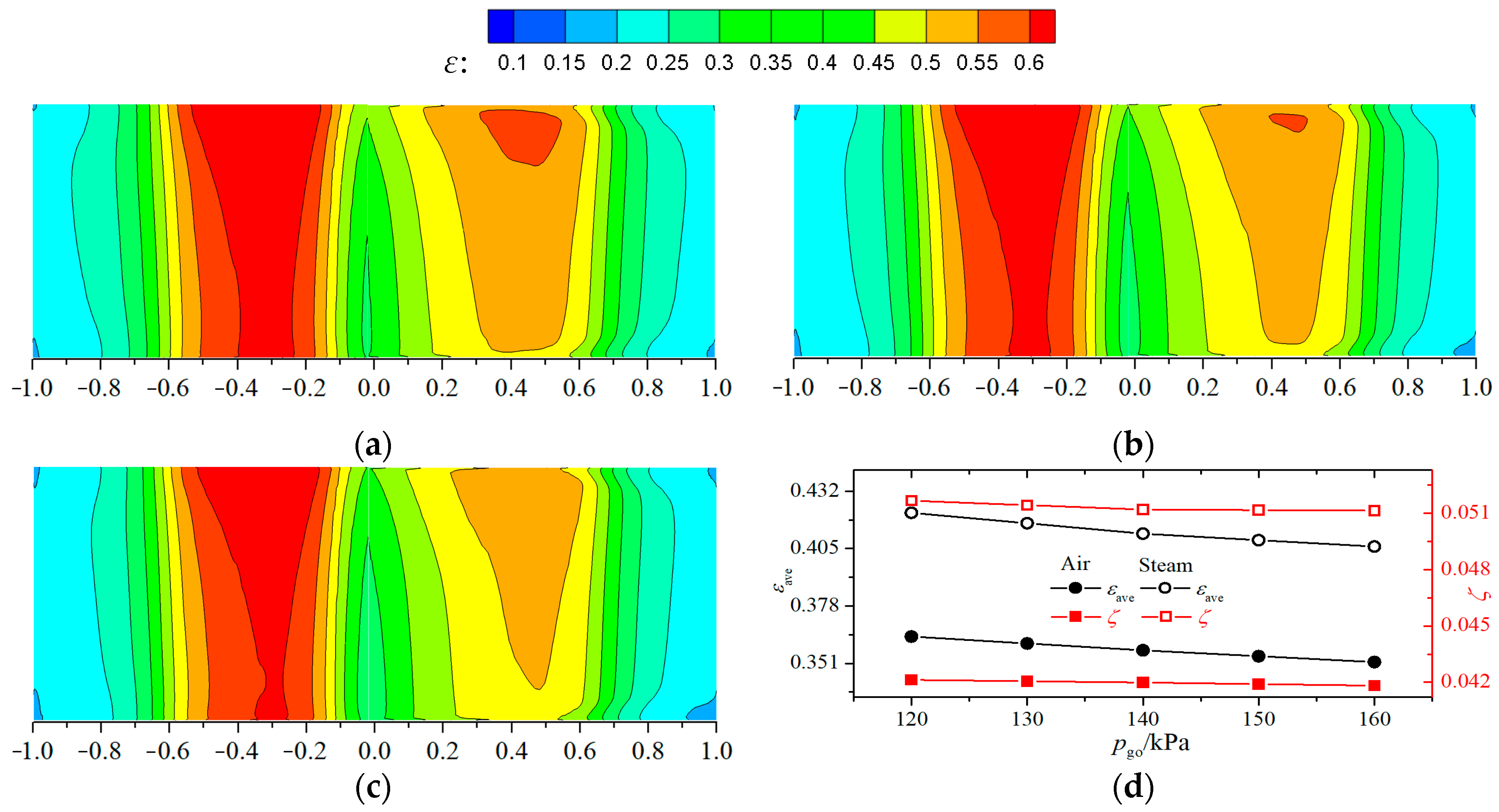
3.2. Influence of Mainstream Outlet Pressure

Figure 10 presents the influence law of the mainstream outlet pressure on the cooling efficiency distribution of the steam-cooled blade, from Figure 10a–c, it can be observed that when the mainstream outlet pressure changes, the distribution of the surface cooling efficiency of the steam-cooled blade is in the range of 0.26–0.67. When the mainstream outlet pressure increases, the area of the high cooling efficiency area in the middle chord area of the steam-cooled blade slightly decreases, while the area of the low cooling efficiency area in the leading and trailing edges of the blade slightly increases. The area of cooling efficiency region in the leading and trailing edges of the blade increases slightly. The cooling efficiency of the steam-cooled blade surface decreases with the increase of the mainstream outlet pressure, but at the same time the temperature of the blade surface is more uniform, which indicates that the mainstream outlet pressure reduces the temperature non-uniformity of the steam-cooled blade. After calculation, it can be seen that when the mainstream outlet pressure increases from 120 kPa to 160 kPa, the average cooling efficiency of the steam-cooled blade decreases by 3.76% and the temperature non-uniformity decreases by 1.03%. From Figure 10d, it can be known that the mainstream outlet pressure on the average cooling efficiency and temperature non-uniformity of air-cooled and steam-cooled blades have the same effect law, that is, the increase of the mainstream outlet pressure will reduce the average cooling efficiency and temperature non-uniformity of both. From Figure 10d, it is also clear that the steam-cooled blade has higher cooling efficiency and temperature non-uniformity compared with the air-cooled blade at the same mainstream outlet pressure. In the studied parameter range, the average cooling efficiency of the former is higher than that of the latter by about 15.38–16.02%, with an average of about 15.60%; the temperature non-uniformity of the former is higher than that of the latter by about 21.96–22.65%, with an average of about 22.26%.

Figure 10. Influence of mainstream outlet pressure on the distribution of cooling efficiency: (a) p_go = 120 kPa; (b) p_go = 140 kPa; (c) p_go = 160 kPa; (d) Variation law of the mean value.

Figure 10. Influence of mainstream outlet pressure on the distribution of cooling efficiency: (a) p_go = 120 kPa; (b) p_go = 140 kPa; (c) p_go = 160 kPa; (d) Variation law of the mean value.

Figure 11 presents the influence law of the mainstream outlet pressure on the distribution of the dimensionless temperature of the steam cooled blade, from Figure 11a–c, it can be found that when the mainstream outlet pressure increases, the distribution of the dimensionless temperature on the surface of the steam cooled blade is in the range of 0.78–0.92, and the area of the low dimensionless temperature region in the middle chord area of the steam cooled blade is slightly reduced, while the area of the high dimensionless temperature region at the leading and trailing edges of the blade is slightly increased. This indicates that the increase of the mainstream outlet pressure will slightly increase the dimensionless temperature of the steam cooled blade. In addition, from Figure 11a–c, it can be known that the change of the mainstream outlet pressure has a greater effect on the dimensionless temperature of the chordal area in the suction surface of the steam cooking blade compared with other areas. After calculation, it can be seen that when the mainstream outlet pressure increases from 120 kPa to 160 kPa, the average dimensionless temperature of the steam cooled blade increases by 0.52%. From Figure 11d, it can be seen that the average dimensionless temperature of both air-cooled and steam-cooled blade increases with the increase of the main stream outlet pressure, but the steam-cooled blade is about 2.15–2.28% lower compared with the air-cooled blade at the same mainstream outlet pressure, and the average is about 2.20% lower.

Figure 11. Influence of mainstream outlet pressure on dimensionless temperature distribution: (a) p_go = 120 kPa; (b) p_go = 140 kPa; (c) p_go = 160 kPa; (d) Variation law of the mean value.

Figure 11. Influence of mainstream outlet pressure on dimensionless temperature distribution: (a) p_go = 120 kPa; (b) p_go = 140 kPa; (c) p_go = 160 kPa; (d) Variation law of the mean value.

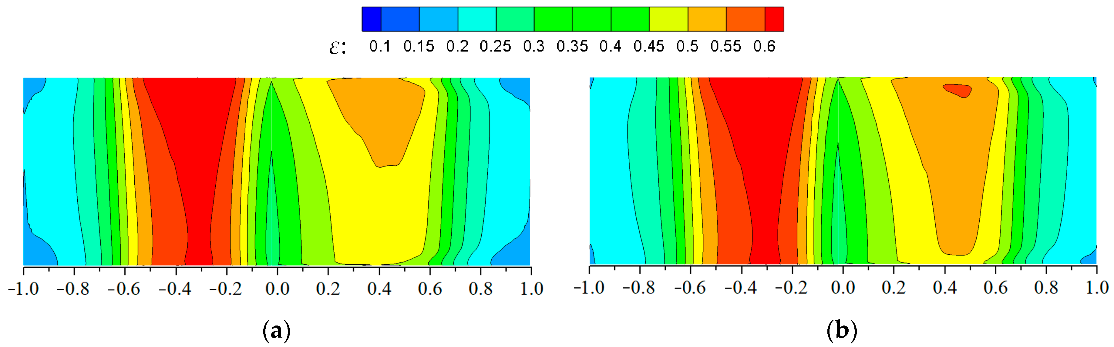
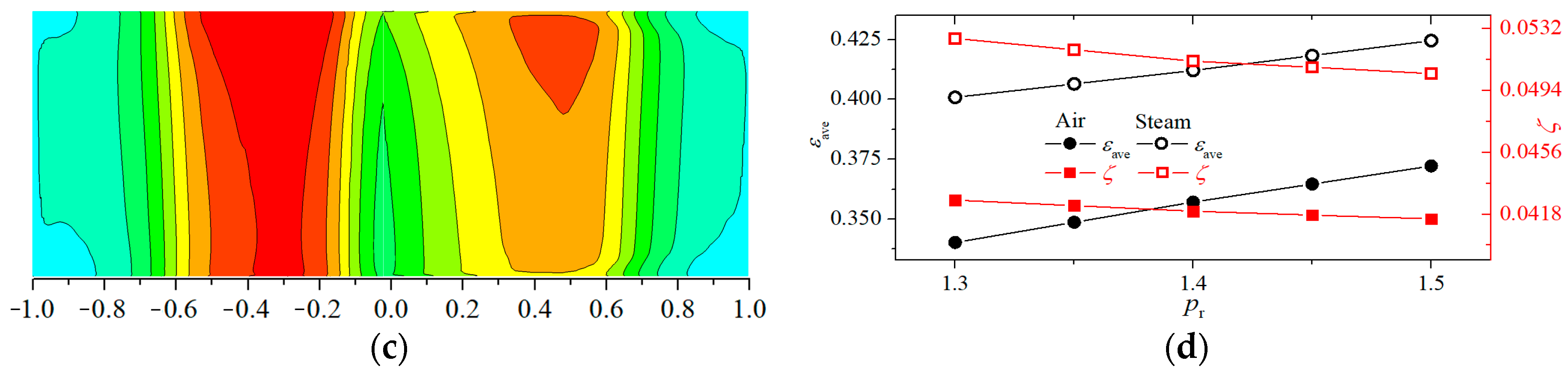
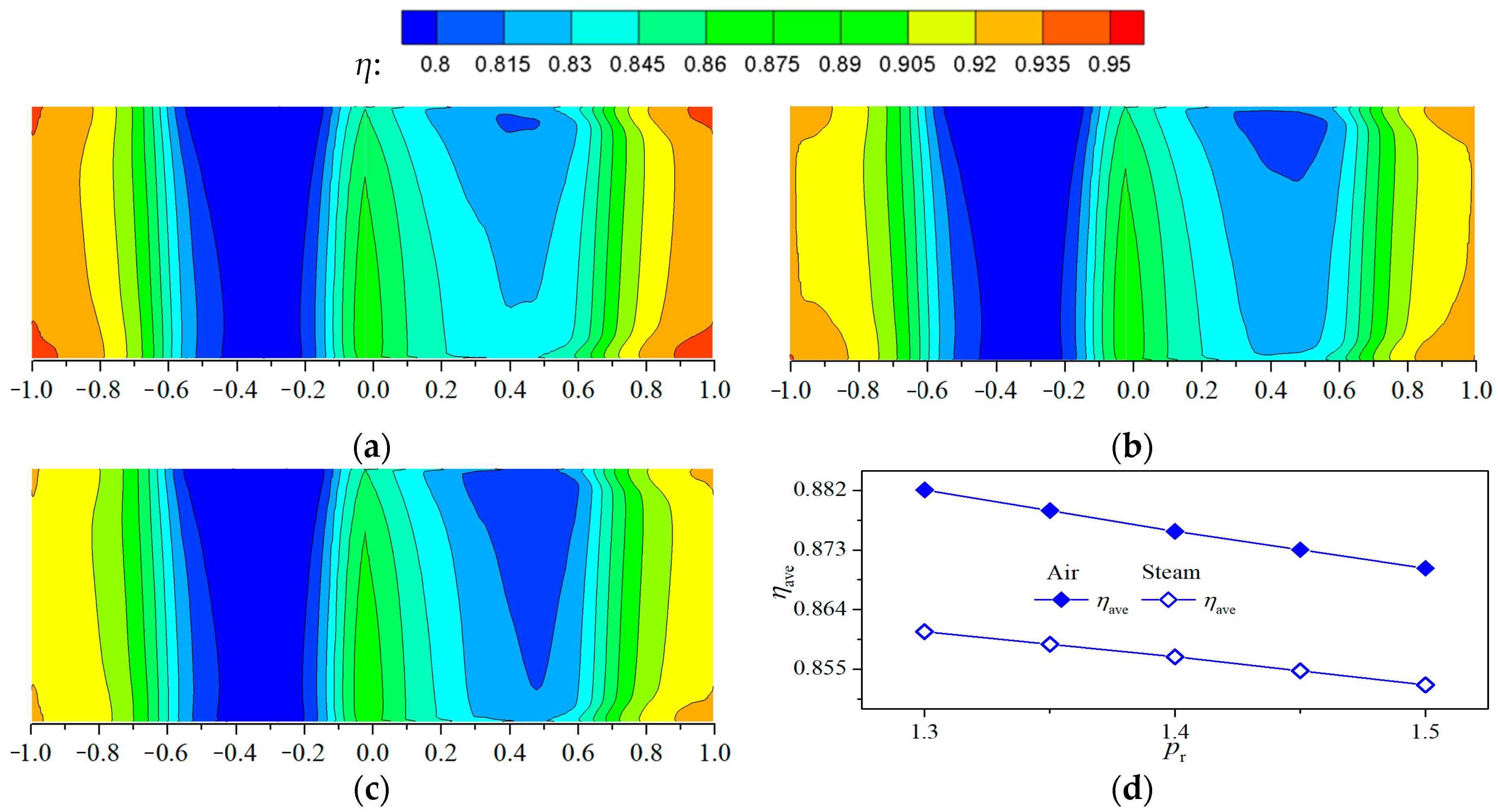
3.3. Influence of Mainstream Inlet to Outlet Pressure Ratio

Figure 12 presents the influence law of mainstream inlet to outlet pressure ratio on the cooling efficiency distribution of the steam-cooled blade, from Figure 12a–c, it can be learned that when the rest of the working parameters are in the middle value and kept constant, the cooling efficiency distribution of the steam-cooled blade surface is in 0.20–0.62 when the mainstream inlet to outlet pressure ratio is 1.3–1.5. When the mainstream inlet to outlet pressure ratio increases, the cooling efficiency of the steam-cooled blade surface increases, that is the area of the low cooling efficiency area of the trailing edge of the steam-cooled blade reduces, and the area of the high cooling efficiency area of the middle chord area of the blade increases, while the cooling efficiency distribution of the leading edge of the blade changes very little. This may be due to the pressure ratio of the mainstream inlet to outlet increase on the blade leading edge of the airflow impact is not large, but it will make the airflow velocity of the blade chord area and trailing edge increase, which will increase the blade surface heat transfer efficiency, thus increasing the cooling efficiency of the blade. In the relative axial chord length −0.2 and 0.9 region blade cooling efficiency increased by about 0.8% and 16.9%, which indicates that the pressure ratio of the mainstream inlet to outlet on the cooling efficiency of the trailing edge of the steam-cooled blade is greater than the leading edge and the middle chord area. In addition, the temperature distribution on the surface of the steam-cooled blade is more uniform with the increase of the pressure ratio of the mainstream inlet to outlet, which indicates that the pressure ratio of the mainstream inlet to outlet reduces the temperature non-uniformity of the steam-cooled blade. The average cooling efficiency and temperature non-uniformity of the steam-cooled blade increased by 5.92% and decreased by 4.09% with the increase of the pressure ratio of the mainstream inlet to outlet, respectively. From Figure 12d, it can be seen that the average cooling efficiency of steam-cooled blade is about 14.06–17.81% higher than that of air-cooled blade in the range of working parameters, with an average of about 15.71% higher; the temperature non-uniformity of the former is about 21.49–23.27% higher than that of the latter, with an average of about 22.21% higher.

Figure 12. Influence of mainstream inlet temperature on the distribution of cooling efficiency: (a) p_r = 1.3; (b) p_r = 1.4; (c) p_r = 1.5; (d) Variation law of the mean value.

Figure 12. Influence of mainstream inlet temperature on the distribution of cooling efficiency: (a) p_r = 1.3; (b) p_r = 1.4; (c) p_r = 1.5; (d) Variation law of the mean value.

Figure 13 presents the influence law of mainstream inlet to outlet pressure ratio on the dimensionless temperature of steam-cooled blade, from Figure 13a–c, it can be observed that when the mainstream inlet to outlet pressure ratio is 1.3–1.5, the dimensionless temperature distribution on the surface of the steam-cooled blade is 0.78–0.93. When the mainstream inlet to outlet pressure ratio increases, the area of the high dimensionless temperature region at the trailing edge of the steam-cooled blade slightly decreases, and the area of the low dimensionless temperature region at the middle chord of the blade increases. while the variation of the dimensionless temperature distribution at the leading edge of the blade is quite narrow. After calculation, it can be seen that when the mainstream inlet to outlet pressure ratio increases from 1.3 to 1.5, the average dimensionless temperature of the steam-cooled blade decreases by 0.93%. From Figure 13d, it can be found that the average dimensionless temperature of both air-cooled and steam-cooled blade decreases with the increase of the pressure ratio of the mainstream inlet to outlet, but the steam-cooled blade is about 2.03–2.43% lower compared with the air-cooled blade at the same pressure ratio of the mainstream inlet to outlet, and the average is about 2.20% lower.

Figure 13. Influence of mainstream inlet temperature on dimensionless temperature distribution: (a) p_r = 1.3; (b) p_r = 1.4; (c) p_r = 1.5; (d) Variation law of the mean value.

Figure 13. Influence of mainstream inlet temperature on dimensionless temperature distribution: (a) p_r = 1.3; (b) p_r = 1.4; (c) p_r = 1.5; (d) Variation law of the mean value.

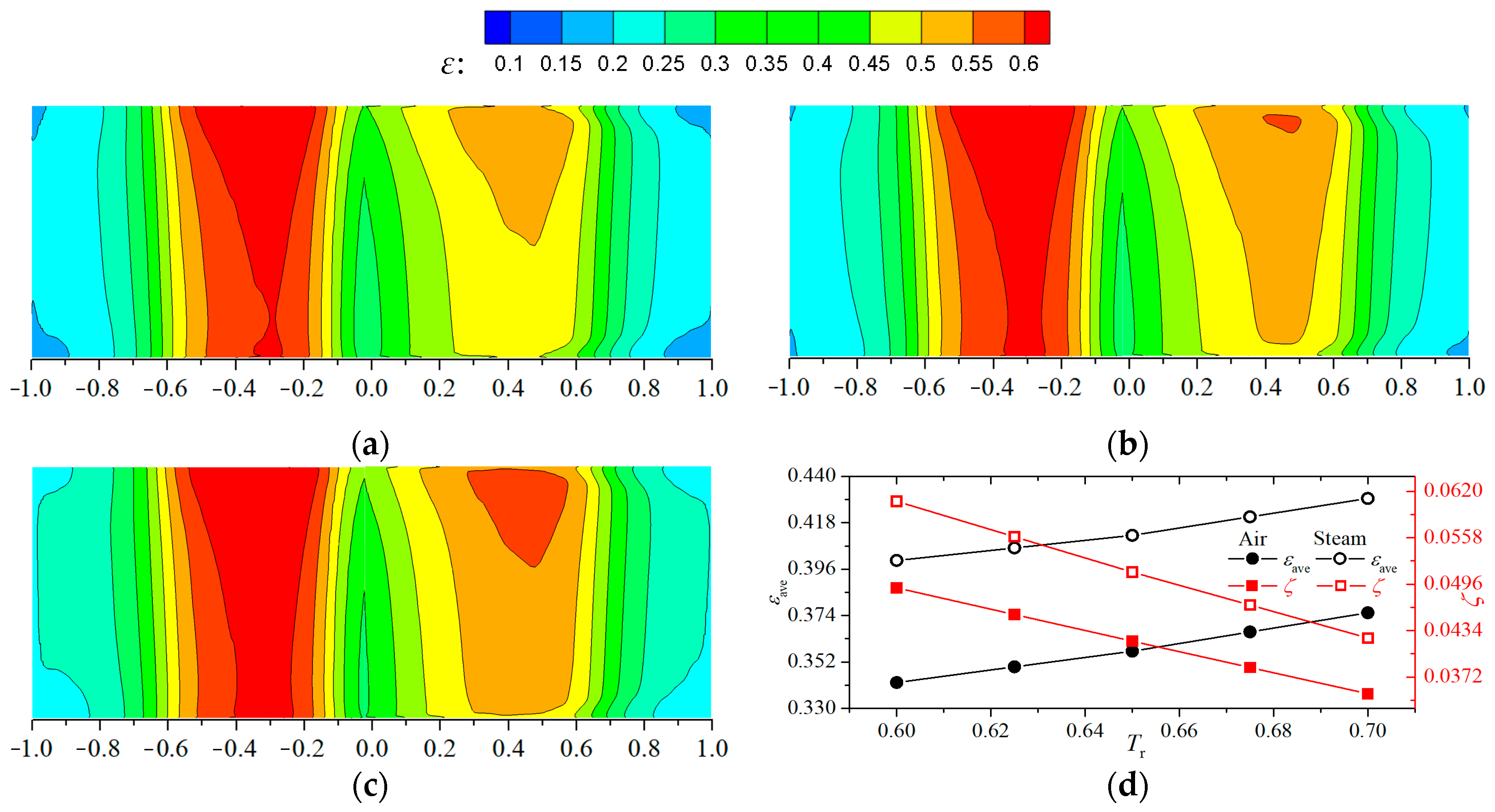
3.4. Influence of Temperature Ratio of Steam to Mainstream

Figure 14 presents the influence law of temperature ratio of steam to mainstream on the cooling efficiency of steam-cooled blade, from Figure 14a–c, it can be shown that when the temperature ratio is in 0.6–0.7, the cooling efficiency distribution of the steam-cooled blade surface is in 0.23–0.63. The cooling efficiency of the steam-cooled blade surface will increase slightly with the increase of temperature ratio of steam to mainstream, the increase of blade trailing edge is about 15%, the increase of middle chord area is about 5–9%, the increase of blade leading edge is about 3–5%. This indicates that the increase of temperature ratio of steam to mainstream has the greatest effect on the cooling efficiency of the trailing edge of the blade, followed by the mid-chord area and leading edge of the blade. In addition, from Figure 14a–c it can also be seen that the blade temperature non-uniformity will be reduced with the increase of temperature ratio of steam to mainstream. After calculation, it can be seen that when the temperature ratio of steam to mainstream increases from 0.6 to 0.7, the average cooling efficiency of the steam-cooled blade increases by 7.35% and the temperature non-uniformity decreases by 30.08%. From Figure 14d, it can be seen that at the same temperature ratio of steam to mainstream, the average cooling efficiency of steam-cooled blade is larger than that of air-cooled blade by about 14.43–16.90%, with an average of about 15.55%; the temperature non-uniformity of the former is higher than that of the latter by about 21.32–23.54%, with an average of about 22.26%.

Figure 14. Influence of mainstream inlet temperature on the distribution of cooling efficiency: (a) T_r = 0.6; (b) T_r = 0.65; (c) T_r = 0.7; (d) Variation law of the mean value.

Figure 14. Influence of mainstream inlet temperature on the distribution of cooling efficiency: (a) T_r = 0.6; (b) T_r = 0.65; (c) T_r = 0.7; (d) Variation law of the mean value.

Figure 15 describes the effect of different temperature ratio of steam to mainstream on the dimensionless temperature distribution of the steam-cooled blade, when the temperature ratio of steam to mainstream is 0.6–0.7, the dimensionless temperature distribution on the surface of the steam-cooled blade is 0.75–0.93. From Figure 15a–c, it can be observed that when the temperature ratio of steam to mainstream increases, the dimensionless temperature on the surface of the steam-cooled blade is all increased. This is due to the fact that increasing the temperature ratio of steam to mainstream raises the temperature of the cooling airflow, and the reduction of the dimensionless temperature on the surface of the steam-cooled blade becomes more difficult as the steam temperature increases. When the temperature ratio of steam to mainstream increases, the dimensionless temperature of the steam-cooled blade increases by about 7.5%, 3.3%, and 1.2% in the relative axial chord lengths of −0.3, 0.05, and 0.9, respectively. This indicates that the influence of the temperature ratio of steam to mainstream on the dimensionless temperature in the chord region of the steam-cooled blade is the greatest, followed by the leading and trailing edge of the blade. After calculation, it can be learned that the average dimensionless temperature of the steam-cooled blade increases by 3.74% when the temperature ratio of steam to mainstream increases from 0.6 to 0.7. From Figure 15d, it can be seen that the average dimensionless temperature of both air-cooled and steam-cooled blade shows an increasing trend with the increase of temperature ratio of steam to mainstream, but the steam-cooled blade is about 1.86–2.58% lower compared with air-cooled blade at the same steam to mainstream temperature, and the average is about 2.20% lower.

Figure 15. Influence of mainstream inlet temperature on dimensionless temperature distribution: (a) T_r = 0.6; (b) T_r = 0.65; (c) T_r = 0.7; (d) Variation law of the mean value.

Figure 15. Influence of mainstream inlet temperature on dimensionless temperature distribution: (a) T_r = 0.6; (b) T_r = 0.65; (c) T_r = 0.7; (d) Variation law of the mean value.

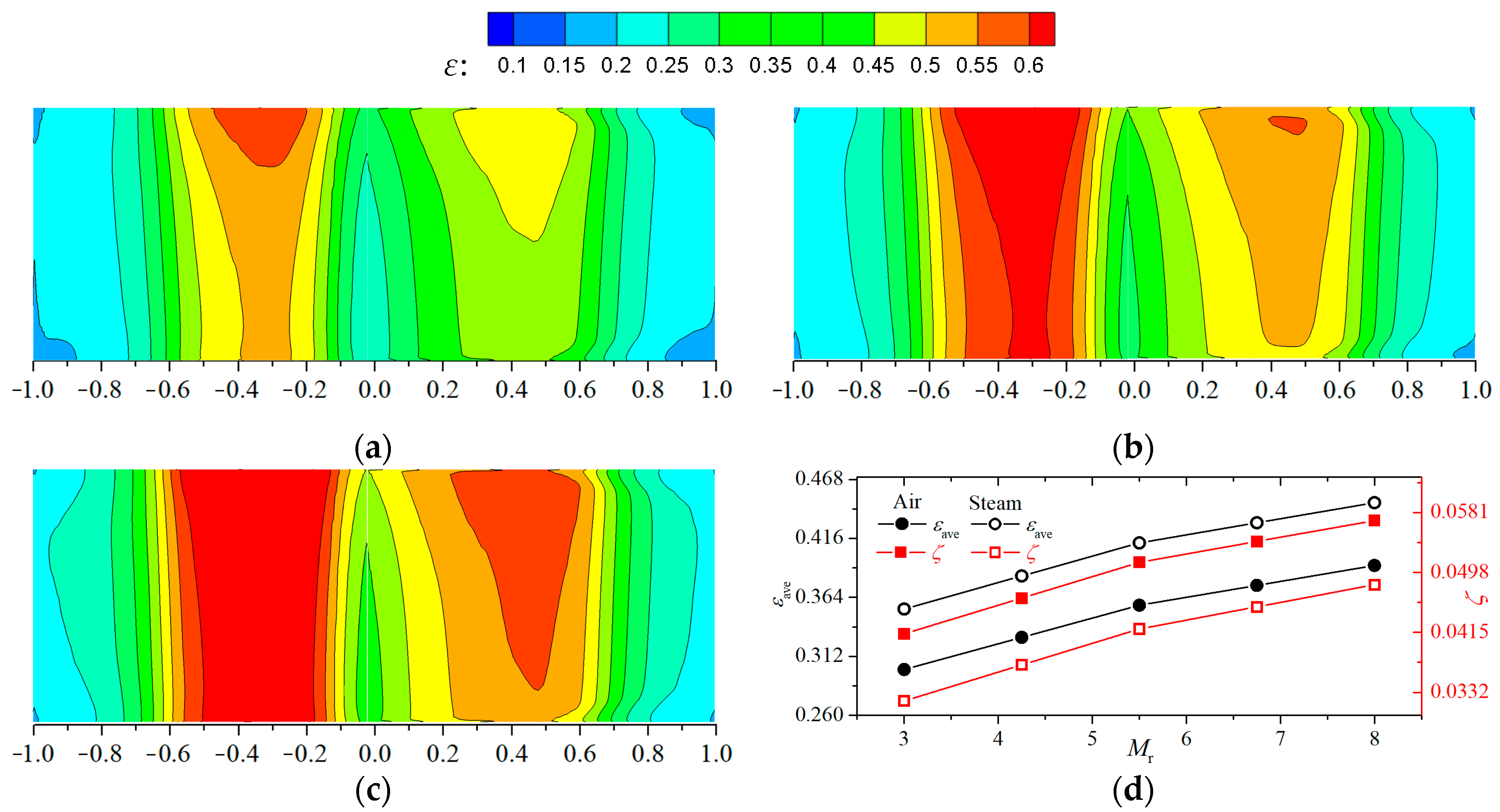
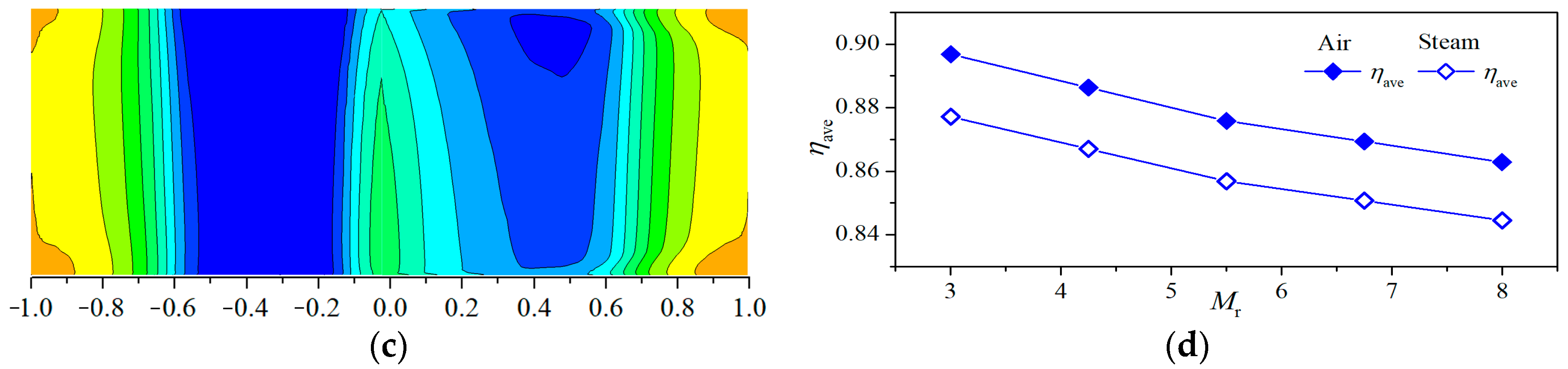
3.5. Influence of Flow Ratio of Steam to Mainstream

Figure 16 provides the effect of the flow ratio of steam to mainstream multiplied by 100, i.e., M_r on the cooling efficiency of the steam-cooled blade, as shown in Figure 16a–c, when M_r is 3, the cooling efficiency distribution on the surface of the steam-cooled blade is in the range of 0.22–0.53; when M_r is 5.5, the cooling efficiency distribution on the surface of the blade is in the range of 0.24–0.62; when M_r is 8, the cooling efficiency distribution on the surface of the blade is in the range of 0.26–0.67. The minimum cooling efficiency of the steam-cooled blade surface increases from 0.22 to 0.26, and the maximum cooling efficiency increases from 0.53 to 0.67, which indicates that the increase of flow ratio of steam to mainstream will greatly improve the cooling efficiency of the steam-cooled blade, which is due to the cooling airflow will carry more heat with the increase of steam flow. At the same time, this will make the temperature distribution of the blade surface more uneven. When the flow ratio of steam and mainstream increases, the cooling efficiency of the steam-cooled blade surface increases, and the increase of the flow ratio of steam and mainstream has the greatest effect on the cooling efficiency of the leading edge of the blade, followed by the mid-chord area and trailing edge of the blade. After calculation, it can be seen that when M_r increases from 3 to 8, the average cooling efficiency of the steam-cooled blade increases by 26.51%, and the temperature non-uniformity increases by 37.99%. From Figure 16d, it can be seen that the average cooling efficiency of the steam-cooled blade is about 14.12–17.72% higher than that of air-cooled blade under different flow ratios of steam to mainstream, which is about 15.68% higher on average; the temperature non-uniformity of the former is about 18.47–29.01% higher than that of the latter, which is about 22.91% higher on average.

Figure 16. Influence of mainstream inlet temperature on the distribution of cooling efficiency: (a) M_r = 3; (b) M_r = 5.5; (c) M_r = 8; (d) Variation law of the mean value.

Figure 16. Influence of mainstream inlet temperature on the distribution of cooling efficiency: (a) M_r = 3; (b) M_r = 5.5; (c) M_r = 8; (d) Variation law of the mean value.

Figure 17 provides the effect of steam-cooled blade dimensionless temperature distribution under different flow ratio of steam to mainstream. It can be seen from Figure 17a–c that when the flow ratio of steam to mainstream is multiplied by 100, i.e., M_r is 3, the dimensionless temperature distribution on the blade surface is 0.81–0.93; when M_r is 5.5, the dimensionless temperature distribution on the blade surface is 0.76–0.92; when M_r is 8, the dimensionless temperature distribution on the blade surface is 0.76–0.91. This indicates that the increase of the flow ratio will greatly reduce the dimensionless temperature on the surface of the steam-cooled blade, and when M_r increases, the dimensionless temperature on the surface of the steam-cooled blade has a large reduction. In the relative axial chord lengths of 0.55, 0.05, and 0.9, the dimensionless temperature of the steam-cooled blade decreases by about 4.7%, 4.2%, and 1.5%, respectively. This indicates that the increase in M_r has the greatest effect on the dimensionless temperature in the chord region of the steam-cooled blade, followed by the leading and trailing edge of the blade. After calculation, it can be found that when M_r increases from 3 to 8, the average dimensionless temperature of the steam-cooled blade decreases by 3.71%. From Figure 17d, it can be noted that the increase of flow ratio of steam to mainstream decreases the average dimensionless temperature of both air-cooled and steam-cooled blades, but the former is lower than the latter by about 2.12–2.19% at the same flow ratio, and the average is about 2.16% lower.

Figure 17. Influence of mainstream inlet temperature on dimensionless temperature distribution: (a) M_r = 3; (b) M_r = 5.5; (c) M_r = 8; (d) Variation law of the mean value.

Figure 17. Influence of mainstream inlet temperature on dimensionless temperature distribution: (a) M_r = 3; (b) M_r = 5.5; (c) M_r = 8; (d) Variation law of the mean value.

4. Analysis of the Results of the Response Surface Model Fitting

4.1. Experimental Design of Working Parameters

Central composite face-centered design (CCF) is a type of central composite design (CCD). It can fit the full quadratic model and obtain a highly accurate response surface model by using fewer sample points. Therefore, CCF was selected for the experimental design in this paper.

Table 3. Central composite face-centered design schemes.

Order	Design Variables					Responses
	Tgi/K	pgo/kPa	pr	Tr	Mr	εave	ζ	ηave
1	710	160	1.3	0.7	3	0.349	0.035	0.898
2	695	140	1.5	0.65	5.5	0.426	0.051	0.852
3	710	120	1.5	0.6	3	0.360	0.048	0.857
4	680	120	1.3	0.6	8	0.432	0.070	0.827
5	710	160	1.5	0.6	3	0.348	0.048	0.862
6	680	120	1.5	0.7	8	0.485	0.046	0.856
7	680	120	1.3	0.7	8	0.457	0.049	0.864
8	695	140	1.4	0.65	5.5	0.412	0.051	0.857
9	710	160	1.5	0.6	8	0.436	0.066	0.825
10	710	120	1.3	0.6	8	0.432	0.070	0.827
11	710	120	1.3	0.7	8	0.457	0.049	0.864
12	710	160	1.3	0.7	8	0.440	0.048	0.870
13	680	160	1.5	0.6	3	0.349	0.048	0.862
14	710	120	1.5	0.7	3	0.398	0.034	0.883
15	680	160	1.3	0.7	8	0.440	0.048	0.870
16	680	120	1.5	0.6	8	0.453	0.067	0.818
17	695	120	1.4	0.65	5.5	0.421	0.052	0.853
18	710	160	1.5	0.7	8	0.467	0.045	0.861
19	710	120	1.3	0.6	3	0.331	0.049	0.870
20	710	160	1.3	0.6	8	0.416	0.069	0.834
21	695	160	1.4	0.65	5.5	0.407	0.051	0.859
22	680	160	1.3	0.6	3	0.320	0.049	0.874
23	710	120	1.3	0.7	3	0.360	0.035	0.895
24	680	140	1.4	0.65	5.5	0.413	0.052	0.856
25	695	140	1.4	0.65	3	0.355	0.041	0.878
26	680	160	1.3	0.7	3	0.349	0.035	0.899
27	710	160	1.5	0.7	3	0.387	0.034	0.887
28	680	120	1.3	0.6	3	0.331	0.049	0.869
29	710	140	1.4	0.65	5.5	0.413	0.052	0.856
30	710	160	1.3	0.6	3	0.320	0.049	0.874
31	695	140	1.4	0.6	5.5	0.399	0.061	0.840
32	695	140	1.4	0.65	8	0.447	0.057	0.844
33	680	120	1.3	0.7	3	0.360	0.035	0.895
34	695	140	1.4	0.7	5.5	0.430	0.043	0.873
35	710	120	1.5	0.6	8	0.453	0.067	0.818
36	680	120	1.5	0.7	3	0.398	0.034	0.883
37	710	120	1.5	0.7	8	0.485	0.046	0.856
38	695	140	1.3	0.65	5.5	0.399	0.053	0.862
39	680	160	1.5	0.7	3	0.387	0.034	0.887
40	680	160	1.3	0.6	8	0.416	0.069	0.834
41	680	160	1.5	0.6	8	0.436	0.066	0.825
42	680	120	1.5	0.6	3	0.360	0.048	0.857
43	680	160	1.5	0.7	8	0.467	0.045	0.861

shows the specific central composite surface design table, which mainly includes the order, design variables and response. Where the design variables include T_g, p_go, p_r, T_r and M_r and the responses include average cooling efficiency ε_ave, temperature non-uniformity ζ and average dimensionless temperature η_ave. After removing 11 duplicate central design points, there are 43 sample points in total.

4.2. Correlation Fitting Based on Response Surface Model

The correlation equations of the average cooling efficiency, temperature non-uniformity and average dimensionless temperature of the steam-cooled blade can obtain the characteristics of the heat transfer of the blade in the range of the working parameters, which is important for the safe operation and performance prediction of the blade. The response surface model (RSM) can obtain an explicit correlation between the operating parameters and the characteristics of the heat transfer of the blade with high accuracy, which is given by the following equations [30,31]:

$$y=B_0+{\displaystyle \sum _{\mathrm{i}=1}^k{B}_{\mathrm{i}}{x}_{\mathrm{i}}+}{\displaystyle \sum _{\mathrm{i}=1}^k{B}_{\mathrm{ii}}{x}_{\mathrm{i}}{}^2+}{\displaystyle \sum {\displaystyle \sum _{\mathrm{i}<\mathrm{j}}^k{B}_{\mathrm{ij}}{x}_{\mathrm{i}}{x}_{\mathrm{j}}+}}\omega$$

(13)

where B₀, B_i, B_ii and B_ij are regression coefficients; x_i and x_j are design variables; y is the response; and ω is the prediction error.

The second-order polynomial response surface model was obtained based on CCF fitting. The specific test design table is shown in Table 3. The design parameters are T_g, p_go, p_r, T_r and M_r and the responses are ε_ave, ζ and η_ave. The coefficients of the response surface model are given in

Table 4. Coefficients of response surface model.

Coefficients	εave	ζ	ηave
B0	0.285	−0.008	0.999
B1	−0.00048	0.000216	0.000188
B2	0.000036	0.000135	0.00018
B3	−1.229	−1.023	0.0413
B4	0.317	−0.0224	−0.2213
B5	0.06165	0.018726	−0.034086
B11	0	0	0
B22	0.000001	0	0
B33	0.694	0.0187	0.1034
B44	−0.0983	0.01049	0.0342
B55	−0.001819	−0.000304	0.000636
B12	0	0	0
B13	0.000106	0.000018	−0.000043
B14	−0.000148	0.000007	0.000051
B15	0	0	0
B23	−0.000043	0.000015	−0.00028
B24	−0.000116	−0.000059	0.000041
B25	−0.000033	−0.000003	0.000011
B34	0.4615	0.00586	0.01224
B35	−0.007777	−0.014006	0.022025
B45	−0.008928	−0.002077	0.003074

.

Figure 18 presents a comparison of the numerical simulation value and RSM predicted value for the sample points of the experimental design of the steam-cooled blade. Figure 18a–c shows the comparison of the two values when the response is average cooling efficiency ε_ave, temperature non-uniformity ζ and average dimensionless temperature η_ave of the steam-cooled blade, respectively. In the figure, the solid black line indicates the numerically simulation values of the sample points, the red scatter indicates the RSM predicted values, and the blue line indicates the ±1% deviation of the numerical simulation values. From Figure 18, it can be seen that the RSM predicted values of the average cooling efficiency ε_ave, temperature nonuniformity ζ and average dimensionless temperature η_ave of the steam-cooled blade are all distributed within ±1% of the numerical simulation values of the sample points, which indicates that the fitted response surface model can well predict the numerical simulated values. The root mean square error RMSE and the coefficient of determination R² were used to evaluate the fitting accuracy of the response surface model [32], and the calculated results are shown in

Table 5. Fitting accuracy of the response surface model.

Evaluation Index	εave	ζ	ηave
RMSE	0.00053	0.00015	0.00023
R2	0.9999	0.9999	0.9999

. As can be seen from Table 5, when the responses are the average cooling efficiency of the blade ε_ave, the temperature nonuniformity ζ and the average dimensionless temperature η_ave, respectively, the RMSE of the response surface model are 0.00053, 0.00015 and 0.00023, which are less than 0.001; the coefficients of determination R² of the response surface model are 0.9999, 0.9999 and 0.9999, respectively, all of which are greater than 0.99. This indicates that the fitted response surface model has smaller errors and higher accuracy.

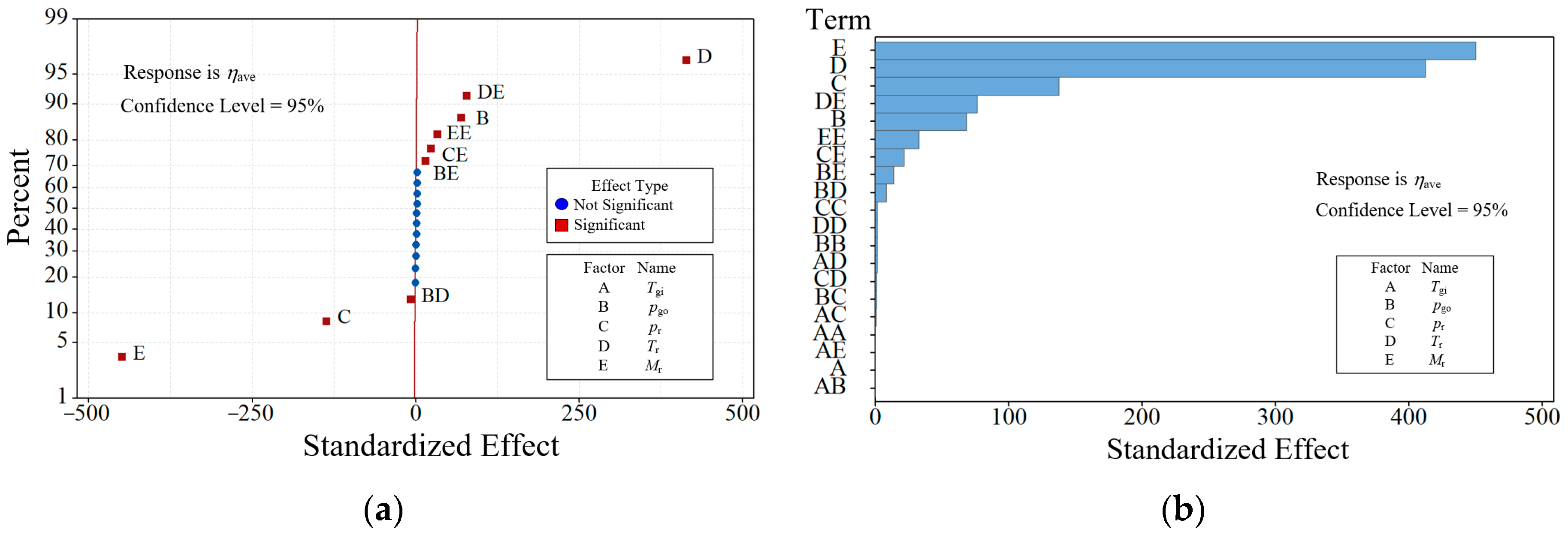
4.3. Significance Analysis of Working Parameters

The central composite design (CCD)-response surface method (RSM) was used to analyze the significance of the design parameters (T_g, p_go, p_r, T_r and M_r) when the responses were the average cooling efficiency ε_ave, temperature non-uniformity ζ, and average dimensionless temperature η_ave of the steam-cooled blade, respectively. The factor effect diagrams for the average dimensionless temperature ε_ave, temperature non-uniformity ζ, and average dimensionless temperature η_ave of the steam-cooled blade are given in Figure 19, Figure 20 and Figure 21, where the Pareto effect and normal effect diagrams are shown in Figure 19a,b, Figure 20a,b and Figure 21a,b, respectively. In the Pareto effect diagram, the positive effects are distributed to the right of the red line and the negative effects are distributed to the left of the red line. In the normal effects diagram, the effects of each factor are arranged in a sequence from small to large, showing the significance of each work parameter. As can be seen from Figure 19, the sensitivity levels of the effective terms for the average cooling efficiency of the steam-cooled blade are M_r, T_r, p_r, p_go, M_r × M_r, p_r × M_r, p_r × T_r, T_r × M_r, p_go × M_r and T_r × T_r in descending order. Where M_r, T_r, p_r, p_r × T_r and T_r × T_r have a positive effect on the average cooling efficiency of the steam-cooled blade, and p_go, M_r × M_r, p_r × M_r, T_r × M_r and p_go × M_r have a negative effect on the average cooling efficiency of the steam-cooled blade. From Figure 20, we can see that the sensitivity levels of the effective terms for the temperature non-uniformity of the steam-cooled blade are T_r, M_r, T_r × M_r, p_r, M_r × M_r, p_r × M_r, p_go, p_go × M_r and p_go × p_r in descending order. Where M_r has a positive effect on the temperature non-uniformity of the steam-cooled blade, and T_r, T_r × M_r, p_r, M_r × M_r, p_r × M_r, p_go, p_go × M_r and p_go × p_r have a negative effect on the temperature non-uniformity of the steam-cooled blade. It can be seen from Figure 21 that the sensitivity levels of the effective terms of the average dimensionless temperature of the steam-cooled blade in descending order are M_r, T_r, p_r, T_r × M_r, p_go, M_r × M_r, p_r × M_r, p_go × M_r and p_go × T_r. Among them, T_r, T_r × M_r, p_go, M_r × M_r, p_r × M_r and p_go × M_r have positive effects on the average dimensionless temperature of the blade, and M_r, p_r and p_go × T_r have negative effects on the average dimensionless temperature of the blade. Among the five working parameters T_g, p_go, p_r, T_r and M_r, M_r is the most significant parameter affecting the average cooling efficiency of the steam-cooled blade, followed by T_r, p_r and p_go. T_r is the most significant parameter affecting the temperature non-uniformity of the blade, followed by M_r, p_r and p_go. M_r is the most significant parameter affecting the average dimensionless temperature of the blade, followed by T_r, p_r and p_go. In addition, T_g has almost no effect on the performance of the steam-cooled blade.

5. Conclusions

In this paper, the cooling performance of the steam-cooled blade, including cooling efficiency, temperature non-uniformity and dimensionless temperature, was studied numerically using experimental design and response surface model, and the relevant empirical formulas were fitted. The main conclusions are as follows:

(1) The empirical formulas obtained using the experimental design and response surface model have high accuracy, and the RMSE of the response surface model are all less than 0.01 and the R² are all greater than 0.99 when the responses are the average cooling efficiency, temperature non-uniformity and average dimensionless temperature of the blade, respectively.

(2) The influence of the mainstream inlet temperature on the cooling performance of the steam-cooled blade is not significant, and the influence of the mainstream outlet pressure is also small. When the pressure increases from 120 kPa to 160 kPa, the average cooling efficiency of the steam-cooled blade decreases by 3.29%, the temperature non-uniformity decreases by 1.03%, and the average dimensionless temperature increases by 0.52%.

(3) When the mainstream inlet to outlet pressure ratio, temperature ratio and flow ratio of steam to mainstream vary from 1.3–1.5, 0.6–0.7 and 3–8, respectively, the average cooling efficiency of the steam cooled blade increases by 5.92%, 7.35% and 26.51%, respectively; the average dimensionless temperature decreases by 0.93%, increases by 3.74% and decreases by 3.71%, respectively; the temperature non-uniformity decreases by 4.09%, 30.08% and improves by 37.99% respectively.

(4) Under the same working conditions, the steam-cooled blade has higher cooling efficiency and lower dimensionless temperature compared with the air-cooled blade, but at the same time the former has higher temperature non-uniformity than the latter. In the research working condition parameter range, the average cooling efficiency of the former is about 14.06–17.81% higher than that of the latter, the average dimensionless temperature is about 1.86–2.58% lower, and the temperature non-uniformity is about 18.47–29.01% higher.

References

1. Xu, L.; Sun, Z.; Ruan, Q.; Xi, L.; Gao, J.; Li, Y. Development Trend of Cooling Technology for Turbine Blades at Super-High Temperature of above 2000 K. Energies 2023, 16, 668. [Google Scholar] [CrossRef]
2. Nourin, F.N.; Amano, R.S. Review of Gas Turbine Internal Cooling Improvement Technology. J. Energy Resour. Technol. 2020, 143, 8. [Google Scholar] [CrossRef]
3. Yeranee, K.; Rao, Y. A review of recent studies on rotating internal cooling for gas turbine blades. Chin. J. Aeronaut. 2021, 34, 85–113. [Google Scholar] [CrossRef]
4. Zhang, L.; Cao, G.; Feng, K.; Jia, Y.; Zhang, Z. Improvement of Multi-Hole Airflow Impingement on Flow and Heat Transfer Characteristics Inside a Turbine Vane Cavity. Appl. Sci. 2021, 11, 9924. [Google Scholar] [CrossRef]
5. Du, W.; Luo, L.; Jiao, Y.; Wang, S.; Li, X.; Sunden, B. Heat transfer in the trailing region of gas turbines–A state-of-the-art review. Appl. Therm. Eng. 2021, 199, 117614. [Google Scholar] [CrossRef]
6. Ngetich, G.C.; Murray, A.V.; Ireland, P.T.; Romero, E. A Three-Dimensional Conjugate Approach for Analyzing a Double-Walled Effusion-Cooled Turbine Blade. J. Turbomach. 2018, 141, 1. [Google Scholar] [CrossRef]
7. Luo, J.; Razinsky, E.H. Conjugate Heat Transfer Analysis of a Cooled Turbine Vane Using the V2F Turbulence Model. J. Turbomach. 2006, 129, 773–781. [Google Scholar] [CrossRef]
8. John, B.; Senthilkumar, P.; Sadasivan, S. Applied and Theoretical Aspects of Conjugate Heat Transfer Analysis: A Review. Arch. Comput. Methods Eng. 2019, 26, 475–489. [Google Scholar] [CrossRef]
9. Prapamonthon, P.; Yooyen, S.; Sleesongsom, S.; Dipasquale, D.; Xu, H.; Wang, J.; Ke, Z. Investigation of Cooling Performances of a Non-Film-Cooled Turbine Vane Coated with a Thermal Barrier Coating Using Conjugate Heat Transfer. Energies 2018, 11, 1000. [Google Scholar] [CrossRef]
10. Nowak, G.; Wróblewski, W.; Nowak, I. Convective cooling optimization of a blade for a supercritical steam turbine. Int. J. Heat Mass Transf. 2012, 55, 4511–4520. [Google Scholar] [CrossRef]
11. Zhu, W.; Wang, J.W.; Yang, L.; Zhou, Y.C.; Wei, Y.G.; Wu, R.T. Modeling and simulation of the temperature and stress fields in a 3D turbine blade coated with thermal barrier coatings. Surf. Coat. Technol. 2017, 315, 443–453. [Google Scholar] [CrossRef]
12. Zhang, G.; Zhu, R.; Xie, G.; Li, S.; SundÉN, B. Optimization of cooling structures in gas turbines: A review. Chin. J. Aeronaut. 2022, 35, 18–46. [Google Scholar] [CrossRef]
13. Liu, Z.; Karimi, I.A. Gas turbine performance prediction via machine learning. Energy 2020, 192, 116627. [Google Scholar] [CrossRef]
14. Abbasi, S.; Gholamalipour, A. Performance optimization of an axial turbine with a casing injection based on response surface methodology. J Braz. Soc. Mech. Sci. 2021, 43, 435. [Google Scholar] [CrossRef]
15. Lakzian, E.; Yazdani, S.; Lee, B.J. Passive control optimization of condensation flow in steam turbine blades. Int. J. Mech. Sci. 2023, 237, 107804. [Google Scholar] [CrossRef]
16. Mahdavi, N.; Mojaver, P.; Khalilarya, S. Multi-objective optimization of power, CO2 emission and exergy efficiency of a novel solar-assisted CCHP system using RSM and TOPSIS coupled method. Renew. Energ. 2022, 185, 506–524. [Google Scholar] [CrossRef]
17. Wang, Q.; Yang, L.; Huang, K. Fast prediction and sensitivity analysis of gas turbine cooling performance using supervised learning approaches. Energy 2022, 246, 123373. [Google Scholar] [CrossRef]
18. Maheshwari, M.; Singh, O. Comparative evaluation of different combined cycle configurations having simple gas turbine, steam turbine and ammonia water turbine. Energy 2019, 168, 1217–1236. [Google Scholar] [CrossRef]
19. Sanjay; Singh, O.; Prasad, B.N. Influence of different means of turbine blade cooling on the thermodynamic performance of combined cycle. Appl. Therm. Eng. 2008, 28, 2315–2326. [Google Scholar] [CrossRef]
20. Xing, J.; Han, S.; Song, Y.; An, N.; Zhou, L.; Li, L.; Zhang, H.; Du, X. Improving internal cooling performance of turbine blade with steam in channel with rhombus-patterned biomimetic ribs: A numerical investigation. Therm. Sci. Eng. Prog. 2023, 40, 101789. [Google Scholar] [CrossRef]
21. Najjar, Y.S.H.; Alghamdi, A.S.; Al-Beirutty, M.H. Comparative performance of combined gas turbine systems under three different blade cooling schemes. Appl. Therm. Eng. 2004, 24, 1919–1934. [Google Scholar] [CrossRef]
22. Wang, W. Efficiency study of a gas turbine guide vane with a newly designed combined cooling structure. Int. J. Heat Mass Transf. 2015, 80, 217–226. [Google Scholar] [CrossRef]
23. Xu, L.; Wang, W.; Gao, T.; Shi, X.; Gao, J.; Liang, W. Experimental study on cooling performance of a steam-cooled turbine blade with five internal cooling smooth channels. Exp. Therm. Fluid Sci. 2014, 58, 180–187. [Google Scholar] [CrossRef]
24. Xi, L.; Xu, L.; Gao, J.; Zhao, Z.; Li, Y. Numerical analysis and optimization on flow and heat transfer performance of a steam-cooled ribbed channel. Case Stud. Therm. Eng. 2021, 28, 101442. [Google Scholar] [CrossRef]
25. Xi, L.; Gao, J.; Xu, L.; Zhao, Z.; Ruan, Q.; Li, Y. Numerical Investigation and Parameter Sensitivity Analysis on Flow and Heat Transfer Performance of Jet Array Impingement Cooling in a Quasi-Leading-Edge Channel. Aerospace 2022, 9, 87. [Google Scholar] [CrossRef]
26. Khan, M.S.; Hamdan, M.O.; Al-Omari, S.A.B.; Elnajjar, E. A comparison of oscillating sweeping jet and steady normal jet in cooling gas turbine leading edge: Numerical analysis. Int. J. Heat Mass Transf. 2023, 208, 124041. [Google Scholar] [CrossRef]
27. Rathore, M.M.; Kapuno, R. Engineering Heat Transfer, Second Edition; Jones and Bartlett Publishers, Inc.: Sudbury, MA, USA, 2010. [Google Scholar]
28. Xu, L.; Shui, L.; Gao, J.; Shi, X.; Wang, W.; Li, X. Investigation on Optimal Allocation of Mass Flow and Direction for Binary Cooling Turbine Test Blades. J. Xi’an Jiaotong Univ. 2012, 46, 7–12+90. (In Chinese) [Google Scholar]
29. Jiang, G.; Gao, J.; Shi, X.; Li, F.; Xu, L. Flow and Heat Transfer Characteristics of the Mist/Steam Two-Phase Flow Cooling the Rectangular Channel with Column-Row-Ribs. Int. J. Heat Mass Transf. 2020, 156, 119737. [Google Scholar] [CrossRef]
30. Zhao, Z.; Gao, J.; Xu, L.; Xi, L.; Li, Y. Numerical simulation on structural parameter optimization of heat exchanger with frustum of a cone. J. Xi’an Jiaotong Univ. 2021, 55, 35–46. (In Chinese) [Google Scholar]
31. Mishra, S.; Sharma, A.; Kumari, A.; Sanjay. Response surface methodology based optimization of air-film blade cooled gas turbine cycle for thermal performance prediction. Appl. Therm. Eng. 2020, 164, 114425. [Google Scholar] [CrossRef]
32. Courand, A.; Metz, M.; Héran, D.; Feilhes, C.; Prezman, F.; Serrano, E.; Bendoula, R.; Ryckewaert, M. Evaluation of a robust regression method (RoBoost-PLSR) to predict biochemical variables for agronomic applications: Case study of grape berry maturity monitoring. Chemom. Intell. Lab. Syst. 2022, 221, 104485. [Google Scholar] [CrossRef]
Figure 1. Experimental schematic diagram of the steam-cooled blade.
Applsci 13 06625 g001
Figure 2. Cascade channel and the experimental blade: (a) Cascade channel; (b) The experimental blade and its cooling structure.
Applsci 13 06625 g002
Figure 3. Numerical model of the steam-cooled blade channel.
Applsci 13 06625 g003
Figure 4. Mesh model of the steam-cooled blade channel: (a) Fluid domain mesh; (b) Solid Domain Mesh.
Applsci 13 06625 g004
Figure 5. Numerical method validation of the steam-cooled blade channel: (a) Local cooling efficiency distribution; (b) Average cooling efficiency.
Applsci 13 06625 g005
Figure 6. Temperature distribution on the blade surface: (a) suction surface of the blade; (b) pressure surface of the blade.
Applsci 13 06625 g006
Figure 7. Surface streamline of the blade: (a) suction surface of the blade; (b) pressure surface of the blade.
Applsci 13 06625 g007
Figure 18. Comparison between numerical simulation value and RSM predicted value: (a) Average cooling efficiency; (b) Temperature non-uniformity; (c) Average dimensionless temperature.
Applsci 13 06625 g018aApplsci 13 06625 g018b
Figure 19. The factor effect diagram of εave: (a) Pareto effect diagram; (b) Normal effect diagram.
Applsci 13 06625 g019
Figure 20. The factor effect diagram of ζ: (a) Pareto effect diagram; (b) Normal effect diagram.
Applsci 13 06625 g020
Figure 21. The factor effect diagram of ηave: (a) Pareto effect diagram; (b) Normal effect diagram.
Applsci 13 06625 g021