Detection of HTTP DDoS Attacks Using NFStream and TensorFlow

Abstract

This paper focuses on the implementation of nfstream, an open source network data analysis tool and machine learning model using the TensorFlow library for HTTP attack detection. HTTP attacks are common and pose a significant security threat to networked systems. In this paper, we propose a machine learning-based approach to detect the aforementioned attacks, by exploiting the machine learning capabilities of TensorFlow. We also focused on the collection and analysis of network traffic data using nfstream, which provides a detailed analysis of network traffic flows. We pre-processed and transformed the collected data into vectors, which were used to train the machine learning model using the TensorFlow library. The proposed model using nfstream and TensorFlow is effective in detecting HTTP attacks. The machine learning model achieved high accuracy on the tested dataset, demonstrating its ability to correctly identify HTTP attacks while minimizing false positives.

1. Introduction

In today’s digital world, cybersecurity has become a key concern for individuals, businesses and organizations. As the number of online threats and attacks continues to grow, it is essential to implement effective security measures to protect sensitive information and prevent attacks in cyberspace. Distributed Denial of Service (DDoS) attacks are among the most common and damaging cyber attacks, as they can disrupt the normal operation of HTTP networks, resulting in financial losses and reputational damages. DDoS attacks involve multiple computers or devices flooding a targeted website or an entire network with requests [1]. As a result, the network becomes overloaded and unavailable to users. In works focused on the detection of DDoS attacks, the authors describe the methods of DDoS attacks that can be used. They also point to the fact that the power of DDoS attacks grows exponentially with time [2,3]. Typically, these attacks are launched by botnet networks of infected computers, remotely controlled by cyber criminals. DDoS attacks can be particularly damaging to HTTP networks, which are widely used to access and share information online. To detect anomalies and DDoS attacks, researchers propose several methods, such as the implementation of statistical methods to detect attacks, and the implementation of IPS/IDS systems and also the possibility of using machine learning to detect an attack. In one such work, the authors described various methods of detecting DDoS attacks using machine learning, such as creating a machine learning model using the SVM algorithm. However, in our opinion, only a small amount of data was used to create the model. The accuracy of the model reached over 98%, but when using real threats, the results did not reach such accuracy, due to the lack of additional information [4,5,6,7,8].

A critical step in preventing DDoS attacks on HTTP networks is to detect them before they can cause any significant damage. In recent years, several methods and techniques have been developed to detect DDoS attacks on HTTP networks so that organizations can take immediate action to mitigate the impact of these attacks. One of the most effective methods of detecting HTTP DDoS attacks is traffic analysis. This involves analyzing network traffic patterns and looking for traffic anomalies or spikes that may indicate a DDoS attack [9,10]. DDoS attacks often involve sudden spikes in traffic from multiple sources, making them easier to detect through traffic analysis. Another method of detecting HTTP DDoS attacks is to analyze the server logs. When analyzing server logs, the goal is to identify unusual traffic patterns, such as sudden spikes in the number of requests from a particular IP address or sudden spikes in traffic to a particular URL [11,12,13].

We consider the lack of various technologies aimed at detecting incidents in a relatively quick time to be important gaps in the research. The time taken to detect incidents depends on the detection capabilities of the machine learning choice, the creation of the model, the choice of technology for data analysis, and also on the size and quality of the data sample. By implementing our own data source, we wanted to focus on detecting attacks in a faster time. This problem is solved in a large number of works focused on cyber security [2,4,14,15].

Other ways of detecting DDoS attacks include the use of intrusion prevention systems (IPSs) and intrusion detection systems (IDSs) [16,17,18]. An IPS monitors network traffic and automatically blocks traffic that is considered malicious, while an IDS alerts security personnel to potential security threats. The IDS and IPS systems can be combined to detect HTTP DDoS attacks [16,19,20]. An IDS can analyze network traffic to find patterns that may indicate a DDoS attack, such as a large number of requests coming from a single IP address or an unusual amount of traffic from a particular region. Once the IDS detects a potential DDoS attack, the IPS can automatically block traffic from problematic IP addresses or take other appropriate mitigation measures. Another option is the implementation of the results from IPS and IDS systems using machine learning. These methods use the IDS system in the process of detecting DoS and DDoS attacks using a hybrid configuration. This configuration combines the use of machine learning and IDS systems into one whole. However, IDS and IPS systems are not the only systems that can be used to detect and prevent DDoS attacks on HTTP networks [14,21,22,23]. For example, network administrators can monitor network traffic and look for unusual traffic spikes or unusual request patterns. Alternatively, various web application filters (WAFs) can be used to filter out malicious traffic and prevent attacks against web applications. In addition to the above, machine learning algorithms and artificial intelligence (AI) techniques can also be used to detect HTTP DDoS attacks [24,25,26,27]. These advanced techniques can identify patterns in network traffic and behavior that indicate a DDoS attack and can alert organizations to take immediate action to mitigate the threat.

The goal of this paper is to review the current state of machine learning research in network traffic analysis and its potential applications in various aspects of network anomaly detection. In this work, we focused on the creation and testing of a machine learning model to achieve an anomaly detection success rate of over 90% and which is not time and computationally demanding for training. We also focused on the design of a model that could be distributed in the CLOUD environment. As part of the work, we tried to improve the parameters of the existing models in order to achieve better accuracy, and we also tried to increase detection accuracy by designing our own dataset. The routing analysis of network traffic dealt with the HTTP protocol, which is the most vulnerable to DDoS attacks on networks.

Another point we focused on in this work is the creation of our own dataset that contains a large amount of information describing the dataset. As described in various works, the most important element of research is the creation of a sufficiently large and accurate dataset [28,29,30,31]. The benefit is the verification and creation of a methodology to create models where it is possible to implement new attack samples over time [32,33].

2. Background and Related Work

The definition of DDoS attacks varies from source to source. This type of attack can be defined as the use of an extremely large volume of packets by an attacker against his/her target through the mutual cooperation of a large number of distributed systems connected to the Internet as shown in Figure 1 [34].

According to this definition, users are denied legitimate access to the target system by consuming the entire network bandwidth and an excessive amount of system resources. Considering the business aspect of DDoS attacks, as described by Yoon [35], these attacks are carried out using remotely controlled external computer botnets to launch attacks on the critical online services of companies on the Internet. Currently, there are several types of advanced DoS attacks, namely, UDP Flood, ICMP Flood, TCP Flood, HTTP Flood and HTTPS Flood [3,8,36,37,38]. We can group them based on their protocols, such as UDP, TCP, HTTP and ICMP attacks. An attack can be easily classified, based on the methods used. DoS attacks have a wide range of methods used. However, they usually have similarities that flood the network with packets [39].

When comparing the most used machine learning methods in other works [3,8,31,33], the attack was divided into four points. The first point is the attacker himself or herself, and the second point is the victim. The third point represents the hosts that generate a large number of requests towards the target of the attack. The last point is the target of the attack. If all these points are met, the attack is successful. The goal is to eliminate the attack in the phase where the attacker is still choosing where to attack. In analyzing and comparing the research efforts, we chose to focus on the use of machine learning, which can successfully detect any anomalies that arise. Within the comparisons, we focused on two points by which we evaluated the models. The first aspect was the accuracy of the model to react to the anomalies that arose, and the second aspect was the speed with which the given model can be trained for new threats. Within our analysis, we dropped the RNN, CNN, KNN, SVM, DBSCAN, DGN, Q-Learning models. In the analysis of machine learning, the focus was further on the use of RNN and CNN algorithms, where the detection success was above 94% in the papers. The authors described these algorithms as the most suitable for classifying network flows. During the analysis, we also considered special types of networks, such as LTSM networks, and also other combinations of LTSM-NB, CNNLTSM, from papers wherein the authors describe LTSM models as advantageous in tasks where it is necessary to implement a longer time dependence of data, which increases accuracy and speed [3,8,31,33,39,40,41,42,43]. With a DDoS attack, it is necessary to focus on a longer period of time for the given attack. These attacks can be carried out in two ways [34,44,45]:

• Draining system resources by consuming all allocated bandwidth and system resources.
• Finding and triggering a failure in the targeted system. Most commonly, this means finding vulnerabilities in application servers and operating systems. These vulnerabilities are then exploited to deny access or to cause damage to the attacked application server.

Authors of scientific research papers place the greatest emphasis on creating the right dataset that contains the necessary number of samples. The authors present the possibilities of creating a dataset of different sizes and properties using chi2, information retrieval scores, backward elimination and other methods. They also focus on KNN models that have been compared using different datasets. They used KNN models and optimized the “K” value for different algorithms. While for DS00_Full they achieved a detection accuracy of 92.95%, for DS02_Chi2 93.08%, DS03_IG 93.36%. When comparing these results, it can be stated that the accuracy of machine learning can be increased by changing the dataset or by adding additional samples and information. In the studies the kinds of attack which can be carried out in a given network were also addressed. This data affects the accuracy of the KNN network, which can lead to false detection, as described in the research conducted by the given authors [31,33,34,46,47]. These most common attacks are described in Figure 2, which shows the share of DDoS attacks on the three layers of the OSI model. According to an Arbor Networks report, the most commonly used DDoS attack methods include SYN flood, DNS flood, and Smurf attack techniques [34]. This report also shows that the frequency of attacks has increased by more than 83% in the last three years. Attackers looking to maximize bandwidth usage launch a UDP flood attack, which can quickly and efficiently overwhelm the system resources of the target network [48].

Figure 3 shows the percentages of the most common network attacks. The most common attack type is UDP flooding, accounting for up to 56% of all detected attacks. The second most common type of attack is TCP flooding. This type of attack is mostly directed against web and application servers [49,50].

Of the attack techniques described above, TCP flood and UDP flood can be used to attack HTTP services. These attacks can be used to exploit the vulnerabilities of the particular web server or to consume all of the allocated bandwidth. New HTTP protocols allow communication using UDP to speed up data transfer. One such protocol is the new HTTP V3 QUICK protocol, which allows a portion of the data to be sent over UDP, i.e., without verification of the delivery of the affected packets [51]. As shown in Figure 3, the proportion of such attacks can be as high as 74%. This service is the most vulnerable because it allows the execution of a large number of applications with a web interface with which users interact [52,53]. From the point of view of machine learning, KNN and RNN methods are based on already available works. According to Priya’s work [54], which used KNN methods, algorithms, Naïve bayes, K-means clustering and Random Forest achieved almost absolute success. Authors Shurman, Khrais and Yateem described, in their work, the possibilities of detecting DoS and DDoS attacks using Deep Learning and IDS [14]. The authors managed to achieve attack detection success of more than 99% based on RNN. From the available research, it can be said that the use of RNN and KNN are appropriate in both cases, and it is possible to achieve high accuracy in the detection of DDoS attacks on various components of computer networks, based on a suitably developed and balanced dataset, as well as on the parameters set in deep learning.

Further Research

Increasing the security of various areas of IT is of paramount importance today. As a result, there is a growing need to find new methods and technologies that can identify different types of threats on their own. This is why machine learning has become a popular topic and many researchers have been exploring its potential applications in a number of research areas. One such area is the use of machine learning in networks implementing the HTTP protocol, as machine learning can help optimize network performance, improve network security and respond flexibly to changes in the network [55,56].

In various works [57,58,59], the authors describe the use of machine learning in the optimization of network flows. These methods are used to optimize network traffic that uses a lot of bandwidth or is burdened by a DDoS attack on HTTP protocols. They used a neural network to analyze network traffic data and then used the predictions to adjust network resources in real time. The result was a significant improvement in network performance, with a reduction in response time and an increase in network throughput [57,58,59].

Other research describes the use of machine learning to detect attacks and anomalies. The studies mostly focus on the detection of DDoS attacks where the authors use machine learning and algorithms to detect these attacks. In these papers, the authors describe the use of machine learning in combination with pre-prepared attack samples that serve to train the model. The datasets created in this way can also be expanded with datasets that are output from IPS and IDS tools. This technique is described in the articles dealing with the automatic detection of attacks and the creation of automated protection against these attacks. All these works agree on the need to use machine learning in the detection of anomalies and attacks on the measured network [60,61,62,63].

Another problem encountered in networks is the method of detecting network traffic. Researchers describe the use of the net flow protocol, which provides data for the creation of the code. However, this protocol depends on the device that is used, so it depends on the device’s router. The most common problem that is described in the works is the absence of a protocol to actually implement machine learning models directly in the detection process. Network traffic sampling is also a problem. This problem was solved by the researchers dealing with Heavy-Hitter by implementing the actual flow device. This flow device enables the implementation of machine learning in the analysis process as well as within its own rules. Researchers opiate the narrowness of machine learning models, such as KNN, SVM, DBSCAN. The most used method is that of KNN networks [64,65,66].

Another use of machine learning in HTTP networks is the detection of XSS attacks and other similar network attacks. The researchers describe the use of machine learning algorithms to detect these attacks from selected LOG files that record user accesses to the system’s WEB interface. Such information can extend protection and block potential attackers who can bypass basic protection. The papers also describe the possibility of detecting these attacks using byridic detection models. The researchers proposed the use of the ABC–AFS system, which implements the advantages of IDS and machine learning. The work describes the use of hybrid classification methods based on Artificial Bee Colony (ABC) and Artificial Fish Swarm (AFS) algorithms. Fuzzy C-Means Clustering (FCM) and Correlation-based Feature Selection (CFS) techniques are used to divide the training data set, and the tame data set is removed, as it is irrelevant [67,68,69].

The rapid development of 5g technologies also leads to the rapid spread of DDoS attacks in 5g network environments. The work “Composite and efficient DDoS attack detection framework for B5G networks” [70] describes the narrowing of machine learning for the detection of DDoS attacks taking place in 5G networks. The work describes the use of the DNN network in the detection of these attacks in four scenarios, where the measurements achieved accuracy ratings ranging from 71% to 99%.

There are several types of models that are relevant when analyzing the possibility of creating machine learning. Each of the possible models is designed for different implementation options. Based on research of possible models, it is possible to use SVN, RNN, DQN, LSTN, LSTN-NB, 3LTSN, CNNLSTM and other models. Based on a comparison of studies and the successful use of models, we focused on three models, namely 3LTSN, CNNLTSN, LTSN. In

Table 1. Performance Comparison among Different RNN models.

Model	Error Rate	Accuracy	Precision	F1
LSTM	2.004%	97.996%	98.108%	97.997%
CNNLSTM	4.108%	95.896%	97.534%	95.831%
3LTSN	3.505%	96.495%	97.688%	96.437%

a comparison of the performance and accuracy of these models is provided [67,71,72,73,74].

In other studies, [75,76], the focus was on LSTM, where researchers tried to compare RNN networks and CNN networks with LSTM cells. The works used models based on combinations of LSTM + NB, LSTM, ANN, CNN-LSTM algorithms. In the works, the authors used P4 as a programming language, with which they were able to analyze network traffic and classify netflows. They also included additional data in the models that the netflow protocol itself did not capture [75,76]. Overall, machine learning has the potential to significantly improve the performance and security of HTTP networks. By analyzing network traffic and identifying patterns, machine learning can help optimize network resources and prevent attacks [73].In the next section, we describe the process of creating a machine learning model and the process of creating a dataset of suitable samples.

3. Methodology

In the theoretical sections above, we defined some of the basic concepts and methods of machine learning used in network analysis. With this theoretical background, a methodology needs to be developed for further research, as is mentioned in the article “Methodology for Detecting Cyber Intrusions in e-Learning Systems during COVID-19 Pandemic” [77]. The methodology of machine learning-based network traffic analysis for anomaly detection can be divided into the following parts [78]:

• Data collection: Collecting relevant data about HTTP network traffic. This can include data from intercepted packets, HTTP application log files and other sources of network traffic data.
• Data pre-processing: The collected data needs to be pre-processed, i.e., cleaned up and normalized. This can include removing any duplicates, filling in missing values and normalizing the data into a consistent format.
• Feature extraction: Relevant features need to be extracted from the pre-processed data. This may include data such as IP addresses, port numbers, protocol types, etc.
• Model training: Building and training a machine learning model from the pre-processed data.
• Model evaluation: Evaluating the performance of the trained model on test data. This can include the use of various metrics, such as model accuracy, F1 score, etc.

3.1. Dataset Creation

This section deals with the design and implementation of machine learning models aimed at detecting HTTP DDoS attacks against network infrastructures. This includes the design of an LSTM RNN algorithm based on six correlated and cooperating layers. Using the nfstream [79] and TensorFlow APIs, the measured network parameters can be analyzed from the PCAP input files, where a netflow matrix is generated and subsequently analyzed. Based on the various parameters, it is possible to define the input data size, and the number of epochs, which affects the speed at which a given model can be trained using the experimental input data [80,81].

3.1.1. Setting up the Environment

Based on the theoretical background and the methodology described above, the first step was to create a system environment in which data collection, data processing and evaluation of the results would take place. The experiment was conducted in two separate environments. The first environment focused on capturing network traffic and storing it in a PCAP data file [82]. The second environment focused on building and training a machine learning model, which was then implemented in the first environment to validate the results. The technical specifications of the first environment is shown in

Table 2. Network traffic capture and store environment.

Component	Value
CPU	4x processor Intel (R) Xeon (R) CPU E5-4610 0 @ 2.40GHz, with a total of 48 cores
RAM	278 GB
GPU	None
Operating System	Ubuntu 20.04 LTS
Network adapter	Intel Corporation 82599ES 10-Gigabit SFI/SFP+

:

The technical specifications of the second environment is shown in

Table 3. Machine learning building and training environment.

Component	Value
CPU	Processor Intel(R) Core(TM) i7-3770 CPU @ 3.40GHz
RAM	16 GB
GPU	NVIDIA Corporation GA106 GeForce RTX 3060 graphics card
Operating System	Ubuntu 22.04 LTS
Network adapter	Internal/Build-in

:

3.1.2. Dataset Design

Choosing the right dataset to build an AI model is the single most important factor influencing the accuracy of a given model. Several types of datasets were selected for use in this paper and were classified into two basic areas, as follows:

• Attack
• Normal

The “Normal” dataset consisted of measured samples used to verify the model used for learning. The “Attack” dataset consisted of attack samples that represented samples of inappropriate network traffic in the network under study. The study “A Hybrid Deep Learning-Based Model for Anomaly Detection in Cloud Datacenter Networks [83]” worked with the same distribution using the DARPA98 dataset [84]. At the start of the model training phase, both datasets were labeled. The samples were labeled with numerical labels as show on

Table 4. Dataset labels according to attack type.

Label	Type
Label 1	SYN flood
Label 2	UDP flood
Label 3	HTTP
Label 4	SCAN port
Label 0	Other

, according to the type of attack included in the given samples:

Classifying these attacks into categories improved the focus on a particular attack when building the model. Each label contained several attack forms, focused on that area. The SYN flood attack consisted of the following patterns:

• Syn_attack1.pcap—this sample contained a record of an attack directed from a device to a server using the High Orbit Ion Cannon (HOIC) application. The attack sample size was 8.3 MB. The attack was then logged using the Wireshark tool.
• Syn_attack2.pcap—this sample contained a SYN attack log, in which multiple machines attacked a server, along with simulation of legitimate traffic. The attack sample size was 14 MB. The attack was then logged using the Wireshark tool.
• Syn_attack3.pcap—this sample contained data from the SDN-DDOS-TCP-SYN dataset [85], created using the mininet generator; it contained the topology of 25 servers independently using the RYU controller. The attack was then logged using the Wireshark tool.

The UDP flood attack consisted of the following samples:

• UDP_attack1.pcap—this sample contained a UDP flood generated against an HTTP service using the Low Orbit Ion Cannon (LOIC) application. The attack was performed from a single device against a single standalone web server supporting HTTP 3. The attack sample was 75 MB in size. The attack was then logged using the Wireshark tool.
• UDP_attack2.pcap—this sample contained data from the “BUET-DDoS2020” dataset [86], where the UDP flood attack contained 125,774 UDP flood attack records. Only this form of attack was extracted from this sample. The attack sample size was 23.1 MB.

The HTTP type attack consisted of several attack samples and variants: HTTP Flood, Slow Read, Slow Post, Slow Get, HULK attack, and Goldeneye attack.

Most of these attacks were concentrated in a single sample, with multiple devices attacking a single server within a single measurement. The samples used were as follows:

• http_attack.pcap—this sample contained a record of an attack against an HTTP server performed using the LOIC system. The attack was performed from a single simulated device against a single HTTP server. The attack sample was 91 MB in size.
• HTTPDoSNovember2021.pcapng—this sample contained a record of network traffic generated by infected devices performing an HTTP DDoS attack. The attack sample was 563 MB in size.
• HTTPDoSJune2022.pcapng—this sample contained a record of network traffic generated by infected devices performing an HTTP DDoS attack. This was an updated version of the previous sample titled “HTTPDoSNovember2021”. This sample contained updated HTTP server attack methods. The size of this sample was 589 MB.

The SCAN port type attack was chosen to increase the efficiency of the given model. This attack method aims to determine the availability of the services of the attacked server. This attack involves launching a large number of automated attacks against a given organization. In most cases, the attacker first scans the server and only then selects the attack method. Therefore, it was useful to add a dataset dealing with network scanning to the machine learning model. To this end, the following samples were used to build the model:

• Scan_nmap—this sample contained a record of network traffic performed by the nmap application; the latter scanned the network containing stations running WEB servers responding on standard (and even non-standard) ports. The web servers used were Apache2 and nginx. The number of servers exposed to this attack was 44, while a network of 255 IP addresses was scanned. The scan log was written by the attacker, so the sample also included attacks against unused IP addresses or IP addresses without HTTP servers. The size of this sample was 7.2 MB.

The second part of the dataset consisted of samples used to validate the model. These samples were labeled Label 0 and contained a sample of real network traffic combined with several types of attacks against the HTTP service. The log of real traffic consisted of four samples of network traffic, recorded on a production network at 1 GB per sample, resulting in a total of 4 GB of real network traffic data. The network traffic was logged using the tcpdump application and the output was then saved to a PCAP file.

3.2. Deep Learning

One of the main areas of machine learning research is supervised machine learning. In this type of learning, a model is trained on a labeled dataset to classify new, previously unknown data or to predict outcomes. This approach is commonly used in image and speech recognition or natural language processing. Another important area of research is unsupervised machine learning, which looks for patterns or structures in unlabeled data [32]. This approach is useful in implementations where machine learning focuses on clustering and dimension reduction. In recent years, deep learning, another machine learning technique, has also gained significant momentum. This approach uses multilayer neural networks with multiple neurons to extract high-level features from the data under study. Deep learning has been particularly successful in image and speech recognition or natural language processing. Machine learning models for image parsing can also be used to analyze network traffic, as machine learning models can interpret data matrices as images, or, alternatively, the data matrices can be defined as mutually independent words. In the study “A Comprehensive Survey on Graph Anomaly Detection with Deep Learning [87]”, a comprehensive overview of available algorithms for Deep-learning was conducted.

According to the authors of “Machine learning and deep learning [88]”, Deep learning is typically made up of several hidden layers that are deeply embedded in network architectures. They usually contain twisted neurons. It is, therefore, possible to perform advanced operations with their help, such as convolution.

Deep learning is an aspect of machine learning that is used in image and text processing. It uses several non-linear layers of processing to extract important objects from the data [89]. Deep learning has now become a method for creating highly accurate systems for classifying objects from data sets. The benefits of deep learning include the following [73]:

• High ability to recognize and classify objects.
• Ability to use high performance GPU cards to accelerate performance. Using these methods, it is possible to reduce the training time of a model to a few minutes.
• High availability of datasets to build custom models for desired situations.

All deep neural models use large amounts of data, labeled with the expected output of the tasks, and multi-layer neural networks for training. The main advantage of these models is the processing of sequential information, where Hidden Markov models and n-gram language models are used. Traditional neural networks assume that output variables are dependent on input variables [89]. However, research has shown that this is not always the case and that the data are not always dependent. This fact is addressed by the use of the Recurrent Neural Network (RNN) model, where the recurrent part is the result of the model’s ability to perform the same task for each element of the data sequence [72]. RNN is capable of modeling sequence data for the needs of similarity recognition and sequence prediction in data. The RNN is built with high-dimensional hidden states that have nonlinear dynamics [90]. Then, the output of the model is highly dependent on the results of the previous step.

The example in Figure 4 shows the way in which the RNN model is trained. The data transfer between training iterations is evident. Thus, an RNN can be thought of as a memory model, where the history of the results of each step in previously processed data can be stored indefinitely. Using the model, each of these values is used to predict the next output of the process.

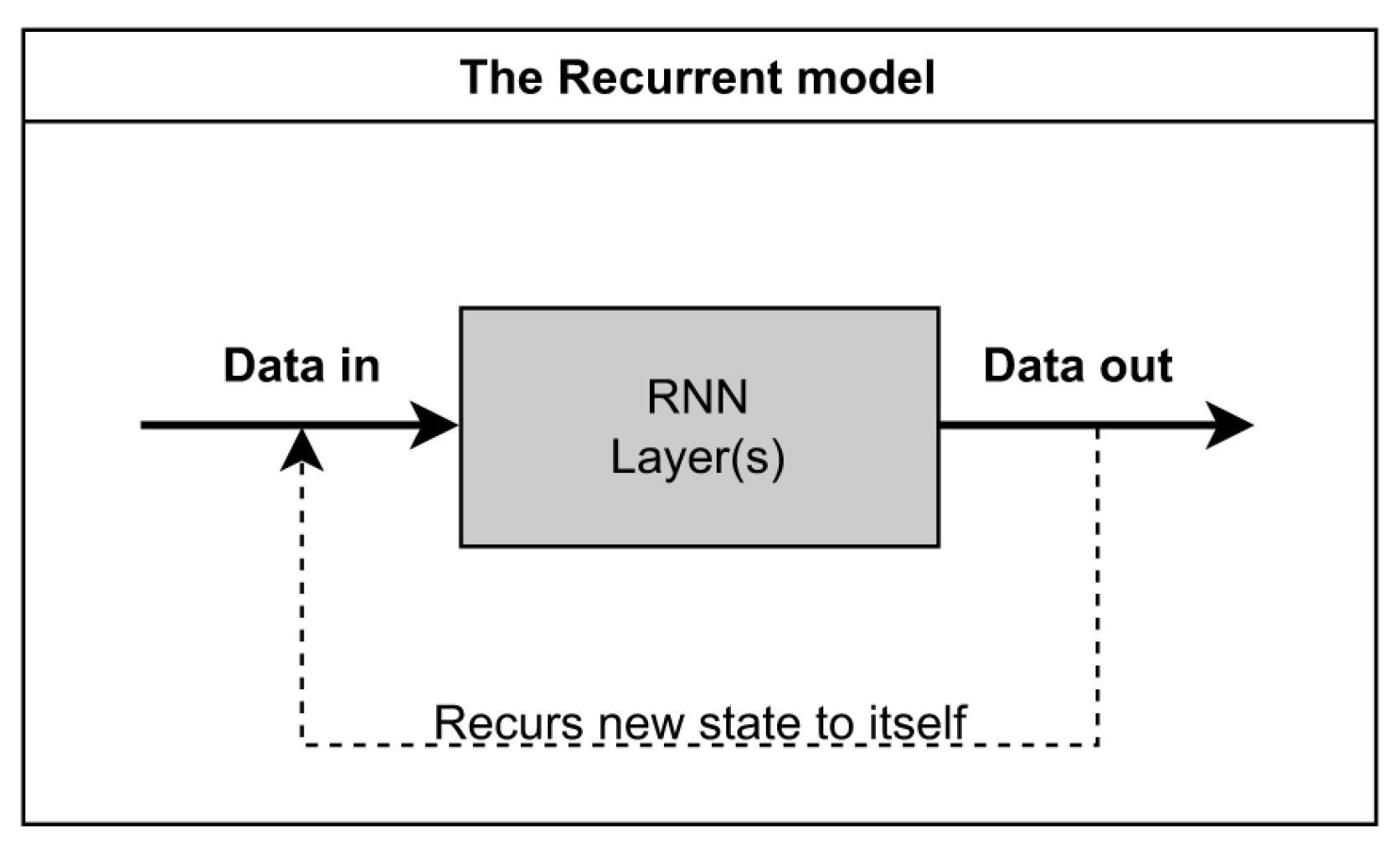
Figure 5 shows a simplified representation of the RNN model, where an iteration block can be represented as an RNN layer. This layer then operates on the input data. The output data from the model is also used in the input calculations. To increase the accuracy, several such layers can be selected in the model to increase the number of iterations.

LSTM RNN machine learning was chosen as the technique for our work because, out of RNN techniques and existing conventional machine learning techniques, LSTM RNN is ranked as the best machine learning technique. This ranking is the result of its ability to learn a longer framework of historical features that enter the algorithm during machine learning training. Unlike other machine learning techniques, LSTM is able to solve the problems associated with a pure RNN with BPTT, by ensuring that the error is kept constant so that the RNN can learn over long time intervals. The RNN LSTM machine learning was able to achieve an accuracy rate of 97.996%, which the older machine learning technique could not achieve [71].

3.3. TensorFlow

TensorFlow is a flexible library for numerical computation using graphs and data flow. With this library, neural networks and other machine learning models can be programmed and trained in an efficient way [89]. The underlying algorithms are optimized to use Nvidia CUDA tools, making it possible to achieve high computational parallelism using multiple devices. The TensorFlow library represents data in the form of tensors. Tensors are multidimensional arrays of data that actually flow as graphs from node to node. In fact, such a graph can be described as a three-dimensional matrix, which need not be strictly mathematically defined [89]. 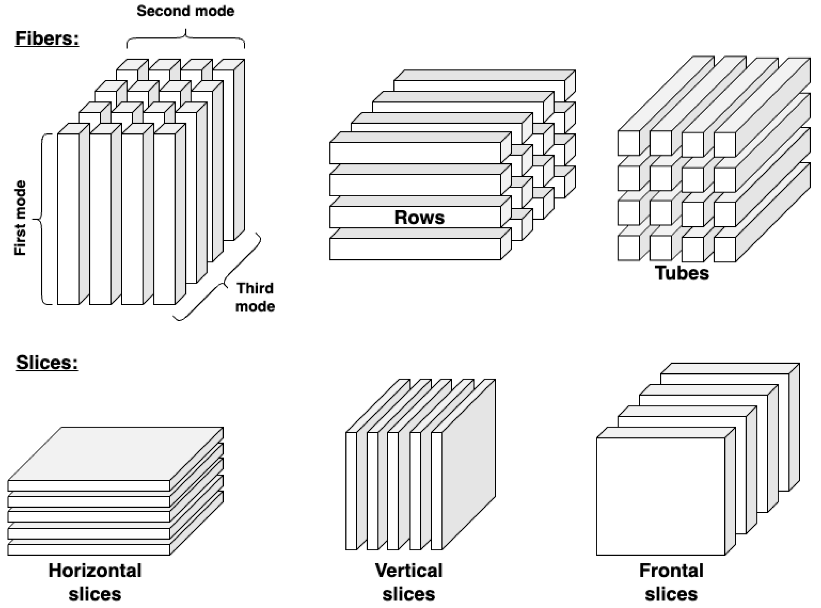Figure 6 shows a vivisection of a tensor. This tensor has multiple inputs in terms of data selection.

Advantages of the TensorFlow library used in this work:

• Great support for different machine learning models and tools for building neural networks.
• The ability to generate any graph from the input data. The system is flexible in choosing the sets from which the data is plotted.
• The system includes predefined mathematical functions for building neural network models.
• Simple support for graphics accelerators is available, which can speed up the training of the model using multiple graphics cards.
• It easily supports various operating systems, including Windows, Linux, Android and iOS.
• It can be used flexibly for research or easy implementation in a production environment.
• Auto-differentiation allows automatic computation of gradient-based machine learning algorithms, such as stochastic gradient descent.
• There is support for the development in Python, in both Python 2 and Python 3 versions.

When developing AI models, it is important to consider metrics that focus on the performance and efficiency of the model. Efficiency is highly dependent on high detection rates and low false positive or false negative rates [91]. However, it is also possible to measure these systems using other methods, such as measuring system power consumption, memory consumption, computational intensity of the models, and other parameters [92]. The N-level detector is usually evaluated in terms of accuracy, where several terms can be defined [21]: True Positive (TP), True Negative (TN), False Positive (FP), False Negative (FN).

$$OverallAccuracy=\frac{TP+TN}{TP+TN+FP+FN}$$

(1)

$$Sensitivity(Recall,TruePositiveRate)=\frac{TP}{TP+FN}$$

(2)

$$Specificity(Selectivity,TrueNegativeRate)=\frac{TN}{TN+FP}$$

(3)

$$Fallout\left(FalsePositiveRate\right)=\frac{FP}{TN+FP}$$

(4)

$$MissRate\left(FalseNegativeRate\right)=\frac{FN}{TP+FN}$$

(5)

$$Precision=\frac{TP}{TP+FP}$$

(6)

$$F1=\frac{2\ast TP}{2\ast TP+FP+FN}$$

(7)

$$Mcc=\frac{(TP\ast TN)-(FP\ast FN)}{\sqrt{(TP+FP)\ast (TP+FN)\ast (TN+EP)\ast (TN+FN)}}$$

(8)

Based on these concepts, the model can be evaluated using different metrics. Based on the aforementioned metrics, designed for the classification component of the detector, it is also possible to perform the analysis globally. Based on the global analysis, the whole system and model is evaluated from the input data, including training, to its output in the resulting system model [72]. For these purposes, the following parameters can be defined:

• Packet Loss Ratio (%)
• Normalized Routing Load (Packets)
• Average End-End Delay (Seconds)
• Average Energy Dissipation (Joules)
• Malicious Drop (Packets)
• False Detection (%)
• Send Buffer Drop (Packets)

When training a model, it is necessary to define how to measure its errors. These errors can be called a loss function, where the goal is to find appropriate parameters that minimize the percentage of errors [72]. The cross-entropy loss function can be defined as follows [93]:

$$L(y,o)=-\frac{1}{N}\sum y_{n}log{o}_n$$

(9)

Architecture for Dataset Analyses

The network traffic datasets prepared for the purpose of building a model using TensorFlow, were stored in PCAP format. However, this format cannot be used optimally to train a model aimed at finding network traffic anomalies. Therefore, the nfstream framework was used as an intermediate framework for data classification. Figure 7 shows the model we used to analyze samples in PCAP format. Pre-processed PCAP files were used as input data, where the NFstream framework allowed the creation of the desired netflow data, which were then tagged with the appropriate labels.

The NFstream framework is a fast python module that provides fast, optimal and flexible data structures designed for analyzing ONLINE or OFFLINE network traffic. This framework is designed to provide a basic building block for network traffic analysis using NDPI classification and using established machine learning models. The advantage is the fast creation and structured reproducibility of the data in sub-applications for research purposes. Another advantage is the ability to perform deep packet analysis, which allows the detection fingerprinting of applications in network traffic, such as TLS, SSH, DHCP, HTTP etc. Network traffic analysis using nfstream was performed with the following parameters:

    streamer = NFStreamer(source=file_path, statistical_analysis=True,

    n_dissections=200)

The options we enabled included the following:

• statistical_analysis—post-mortem flow statistical analysis. This option allows the storage of statistical data from measured network traffic, such as the amount of packets transmitted, minimum and maximum packet size, and other metrics
• n_dissections—the number of packets to analyze when detecting L7 protocols with NDPI. The default size is 20, which is insufficient for measurement purposes and the number of packets analyzed must be increased to improve accuracy.

Once these data had been processed and saved in CSV format, an additional column was added to contain the given LABEL of the desired sample.

3.4. Building the Model

The idea behind this work was to use sequential information, which, using traditional neural networks, assumes that all inputs and outputs of the model are independent of each other. Therefore, we used RNN recurrent neural networks, as these perform training for each element independently, while the result is strictly dependent on the previous results [32]. The basic step in building the model was to unify the data used in the training process. We stored the data converted using nfstream in separate CSV files containing NETFLOW records with the labels added. These records may also contain, in multiple files, different data, produced by the nfstream application. Then, we extracted uniform data from these records and normalized them to have the same number of parameters for each flow solution. If a parameter was missing in any of the samples, the application added the predefined value, i.e., 0. In this way, we ensured that the model building process would work with equally sized matrices of data, thus eliminating the potential risk of inaccuracy or miscalculation. When building the model, we used the following data from the nfstream application:

"src_port","dst_port",

"src2dst_packets", "src2dst_bytes",

"dst2src_packets", "dst2src_bytes",

"src2dst_min_ps","src2dst_mean_ps", "src2dst_stddev_ps", "src2dst_max_ps",

"dst2src_min_ps", "dst2src_mean_ps", "dst2src_stddev_ps","dst2src_max_ps",

"src2dst_min_piat_ms", "src2dst_mean_piat_ms", "src2dst_stddev_piat_ms",

"src2dst_max_piat_ms", "dst2src_min_piat_ms", "dst2src_mean_piat_ms",

"dst2src_stddev_piat_ms","dst2src_max_piat_ms",

"src2dst_syn_packets", "src2dst_cwr_packets", "src2dst_ece_packets",

"src2dst_urg_packets","src2dst_ack_packets", "src2dst_psh_packets",

"src2dst_rst_packets","src2dst_fin_packets",

"dst2src_syn_packets", "dst2src_cwr_packets","dst2src_ece_packets",

"dst2src_urg_packets", "dst2src_ack_packets","dst2src_psh_packets",

"dst2src_rst_packets", "dst2src_fin_packets","src_port","dst_port"

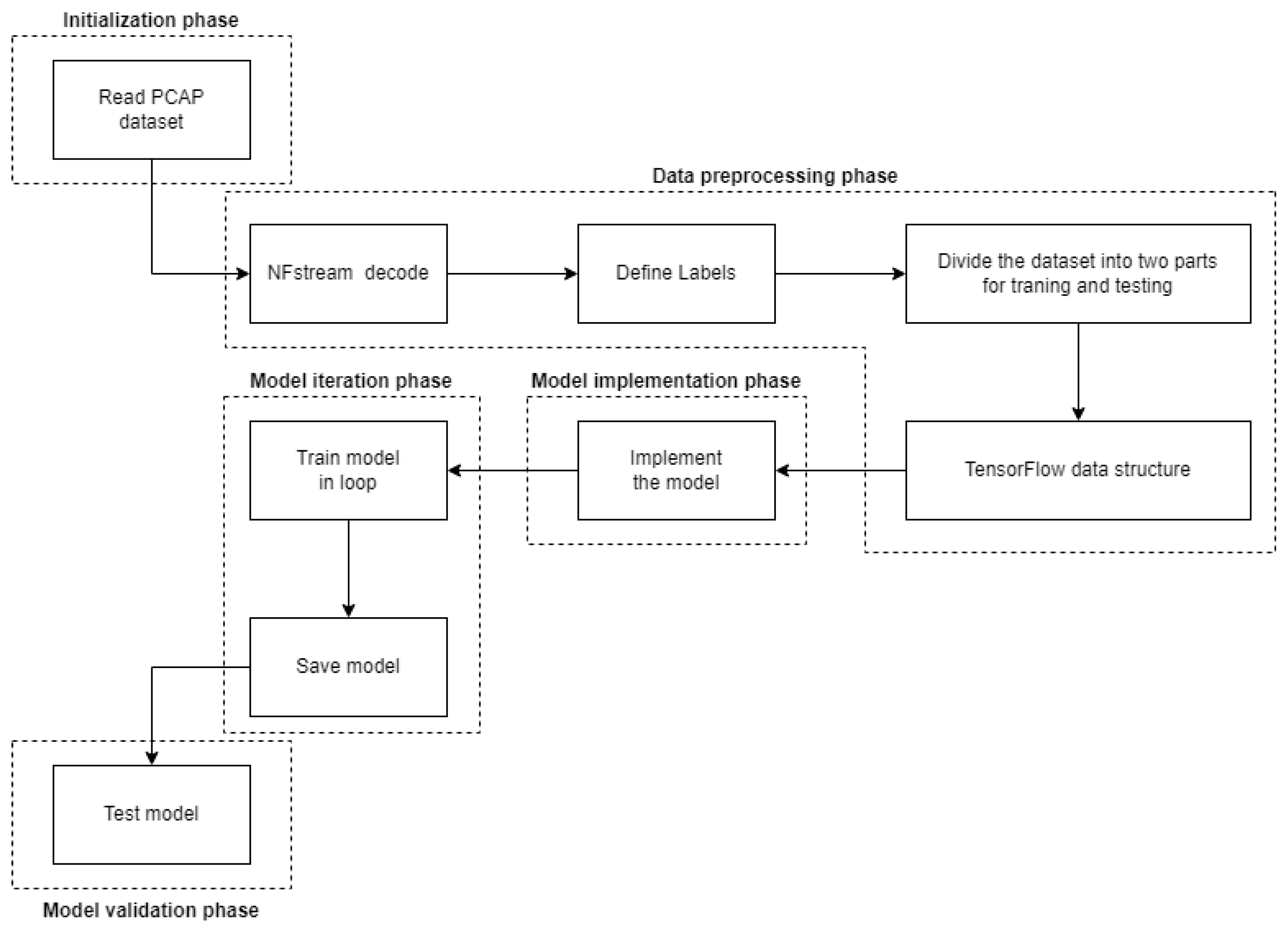
Figure 8 shows the algorithm of the code. It can be divided into five main phases as shown on

Table 5. The TensorFlow algorithm phases.

Phase No.	Phase Description
Phase 1	Initialization phase
Phase 2	Data pre-processing phase
Phase 3	Model implementation phase
Phase 4	Model iteration phase
Phase 5	Model verification phase

:

The initialization phase of the program defines the parameters required by the algorithm, as well as defining the constants required for the subsequent steps of the code. In this phase, we also stored the necessary datasets, which served as model training and validation data, respectively. In the data pre-processing phase, the uniform samples were loaded and categorized into the desired form. The next phase was the model implementation phase, where the implementation of the fivelayer RNN algorithm model took place. In this phase, the weights and biases specified for the model nodes were randomly generated. This was followed by the implementation of the training algorithm, where the algorithm was trained on the required data. This phase depended on the iteration phase, where the learning process was repeated after a certain number of iterations in order to train the given model more accurately. The functionality of the model was then verified. Using test functions, the model was loaded and subjected to test data, comparing the accuracy of the untrained model used in the data analysis process. Parameters on

Table 6. Parameters used in training the experimental model.

Parameter	Value
Epoch	300
Hidden Layers	7
Activation function	ReLu
Optimizer	adam
Classification engine	softmax cross entropy between logits and labels
Neurons on each layer	40
Learning Rate	0.001
Embedding size	2
Class size	17
One hot encoder	Yes
Weights	Random
Biases	Random

were used to train the experimental model:

4. Results

The goal of this experiment was to investigate the efficiency of using a recurrent neural network (RNN) with TensorFlow to detect anomalies in HTTP traffic. Detecting anomalies in network traffic is an important task in identifying potential security threats, such as network intrusions or DDoS attacks. To conduct the experiment, a set of data was collected from a simulated network focusing on the network traffic on the HTTP network. This dataset consisted of normal network traffic and various types of anomalous traffic, including DDoS attacks on HTTP services. The normal traffic was generated by simulating user behavior when browsing web services, while the anomalous traffic was generated by simulating various types of attacks using the tools available in the toolkit described in this paper. The total number of network flows recorded in this experiment was 985,054. The flows were then separated into the training and testing of the model, as is shown in the following

Table 7. Dataset detail.

Total number of transactions	985,054
Number of Normal transactions	394,021
Number of Attack transactions	591,032
Number of test transactions	587,621

.

The RNN was trained on the dataset using TensorFlow. The network consisted of six interconnected layers, with the first layer being the Long Short-Term Memory (LSTM) layer. The LSTM layer was used to capture time-dependent features of the network traffic, while the remaining layers were used to classify the traffic as either normal or anomalous. Figure 9 shows the model accuracy as a function of the number of training epochs. From a training perspective, increasing the number of iterations in the machine learning process leads to an increase in the accuracy of the model. Similarly, the accuracy of the validation of untrained data also increases. During the first 50 iterations, the accuracy of the untrained model increased quite rapidly, as the model validation accuracy increased from 0.72 to 0.79. However, further increases in the number of repetitions did not result in an increase in accuracy.

Figure 10 shows the training loss as a function of the number of training iterations of the model. As can be seen from the results above, the training loss decreased as the number of epochs increased. This indicated that the model was learning and improving over time.

We used the model developed on untrained data in a simulated environment consisting of an nfstream probe that could classify the network traffic based on the machine learning model. This model evaluated packets in real time from prepared smaller samples of various attacks and simulated legitimate network traffic. The sample show on

Table 8. Details of the test dataset.

Details of the test dataset Number of test transactions	587,621
Number of Normal transactions	397,685
Number of Attack transactions	189,936

consisted of 587,621 flows that were subsequently analyzed by this model.

After performing the analysis using nfstream and the developed machine learning model, we were able to classify network traffic in real time, with minimal delay. This classification identified and evaluated each flow separately, and, thus, was able to label a given flow as either suspicious or normal, as early as in the analysis process.

Table 9. Results of the test dataset.

Test1—result of Attack and good transactions	92.85%
Test2—result of Attack transactions	96.54%
Test3—result of good transactions	3.05%

shows the results of the tests performed in the three scenarios set up for the model under study. This test indicated that the system was able to detect 92.85% of the attacks that occurred in the samples containing real-life network traffic and network attacks defined by us. During validation, we also detected false positive attacks. In experiment #3, which consisted of samples containing only legitimate traffic, 3.05% of the samples were classified as an attack. We built this model by combining datasets provided by other researchers and our own samples generated in our simulated infrastructure. The created infrastructure model can easily be enriched with custom samples or other samples. By increasing the amount of samples, the model can achieve higher efficiency rates in anomaly detection.

5. Discussion

This section describes some insights into the experimental findings and selects some findings to illustrate the method used. The detection and machine learning performance was evaluated using various parameters and showed substantial performance compared to existing work conducted in the same field [75,78]. The detection accuracy of the anomaly detection system depends on the correct classification of the attack and normal network traffic. The method used showed an overall classification accuracy of 96.54%. The accuracy of the model differed when measuring three experiments where different types of data were entered. The parameters of machine learning can be changed, mainly by adding the number of training epochs, which increases the accuracy. The problem to be solved during training is the identification and prevention of pre-training of the model. Such pre-training artificially increases the quality of the created model, and the model cannot continue to learn during further training. This error occurs in a large number of studies and should be avoided [94,95].

Another parameter is the introduction of newer samples, which affect the accuracy even when detecting new types of attack.

In a large number of works, the authors use publicly available datasets to create machine learning models, which do not always contain accurate information describing the attack or contain incomplete or anonymized data that then affect the accuracy of the measurements [96,97].

In comparison to the work of other authors, which used detection tools such as netflow, which are most often implemented in routers, we decided to use the nfstream application in our work, which can be used to record network traffic on other devices as well. The differentiating factor in other research works is the possibility of implementing the resulting machine learning model into the network flow analysis process, which makes it possible to easily evaluate network traffic [98,99]. Furthermore, it is possible to apply a granular deployment of this model, where network traffic can be effectively analyzed with the help of smaller probes [100,101]. The price of such an analysis was addressed by authors in other works. Compared to other works, the nfstream application allows you to record parameters other than just basic netflow data [102]. Among the additional parameters, the analysis of network flows using nDPI can be included, where it is possible to detect currently used protocols and applications to categorize network traffic. Such parameters increased the accuracy of the subsequently created model [103].

LTSM was chosen as the machine learning model. Other machine learning models are also described in studies. We would like to emphasize the comparison between two works dealing with the detection of DDOS attacks using machine learning [104].

By implementing the LSTM–BA neural network, it is possible to achieve the desired results. However, as stated in the work “LSTM-BA: DDoS Detection Approach Combining LSTM and Bayes”, it is possible to create a model that combines the advantages of two networks, namely LSTM RNN and Bayes network (LSTM-BA). With this combination, the researchers were able to increase the accuracy of the model by 1.4% in DDoS detection. When compared to the model we tested, this was only a minimal increase in accuracy. In the article, “Self-supervised network traffic management for DDoS mitigation within the ISP domain”, the authors achieved an average detection accuracy of 86% using decision tree, random forest and GBT algorithms. When comparing machine learning algorithms, such as SVC and LG from other works, the method chosen by us achieved the best results. We also achieved similar detection accuracy using TensorFlow, so it could be concluded that the method used was suitable for detecting DDoS attacks [104,105,106].

The table shows the comparison of selected works with our results. The LSTM–BA algorithm achieved a higher result, but, according to the authors of the work, more power and longer time are needed to train it. Our goal was to verify the implementation of the LTSM model with the dataset we created. Compared to this dataset, the difference in model accuracy was minimal [104,107].

The results of the method used for detecting attacks and anomalies using machine learning are applicable for further development. After changing the input datasets, this model can be used to detect types of attacks other than just HTTP DDoS attacks. Further investigation using the current architecture and the created model is advisable to verify its accuracy in detecting other types of attacks, such as attacks on network infrastructure caused by errors in protocols, whereby there is acceleration of attacks from the attacker.

6. Conclusions and Future Perspectives

The primary research described herein focused on anomaly detection in HTTP traffic in computer networks using machine learning and the TensorFlow library. The aim of this paper was to investigate the accuracy of using TensorFlow, a well-known machine learning library, to detect anomalies in HTTP traffic. The results of our work showed that TensorFlow can be used to effectively identify anomalies in HTTP traffic, and that it can be used in conjunction with other machine learning techniques to improve the accuracy of anomaly detection, as described in Section 4 One of the main advantages of using TensorFlow and nfstream for anomaly detection is the ability to analyze large samples of network flow or other complex data structures. This makes them suitable for analyzing network traffic, which is often a time-consuming and complex task. The results of detection accuracy and loss as a function of the number of epochs are described in Section 4. The results are shown in Figure 9 and Figure 10, and it can be observed that the created model achieved a success rate of 92% and 96% in the second experiment. During the measurements, three models were tested, wherein data with different amounts of attack data were entered as test data. The model was able to achieve an accuracy of 92.85% under test conditions when testing normal and abnormal network traffic. This experiment described real network traffic, while experiment No.3 described traffic without attacks, where the model recorded 3.05% of flows as anomalous. The measured dataset contained only data without attacks. The experimental results confirmed the high accuracy of 96.5% classification of LSTM models when using datasets created using nfstream. Compared to other methods of packet analysis, the accuracy was 1.4% lower, to the disadvantage of our created model. The created model and the created infrastructure could be used in the future with essential attributes to increase the accuracy of anomaly detection.

The goal of the experiment was to create a model that, using defined anomaly samples, could detect anomalies in HTTP traffic with high accuracy. This could be implemented in practice for the quick search and detection of anomalies in HTTP network traffic, while the infrastructure could be automated. The results of the measurement in practice showed that the model created from known samples was prone to falsely positive labeled samples. This problem can be minimized by increasing the number of epochs when training the model. Another key advantage of using TensorFlow for anomaly detection is its ability to adapt to emerging patterns of packet behavior in the network. As network traffic patterns can change over time, it is important that the anomaly detection system can adapt and continue to detect anomalies despite the changes. TensorFlow’s ability to learn and adapt to new data patterns makes it well suited to this task. There are also some limitations to using TensorFlow for anomaly detection. One limitation is that TensorFlow requires a significant amount of data to train and test the model. In addition, TensorFlow requires a significant amount of computational resources to run. Despite these limitations, the results showed that TensorFlow can be an effective tool for anomaly detection in HTTP traffic. Its ability to analyze large datasets with complex data structures, as well as its ability to adapt to changing data patterns, makes it suitable for this task. Furthermore, its ability to perform deep learning makes it suitable for detecting complex anomalies.

Our study describes the practical use of a combination of machine learning and nfstream probe, which enables the analysis of network traffic in real operations. The model we propose in this study contributes by creating its own dataset with attacks on the HTTP server. Other researchers can also use this dataset in future works. The created model focuses on increasing the reliability of, and reducing the error rate of, the trained model in detecting attacks in networks. In practice, this solution is suitable, as it can be distributed to servers located in a CLOUD environment. With this distribution of nfstream probes, it is possible to achieve an increase in attack detection performance even without using a special hardware solution. The model can be quickly scaled and supplemented with new attack samples. We also focused on reducing the time needed to train a given model, which, in practice, means that we reduced the time needed to deploy new models.

The work validated the theory by testing and deploying an LSTM model, supporting the results of other researchers who have worked on similar machine learning models. This statement is supported by

Table 10. Comparison of machine learning results.

Model	Accuracy
LSTM	96.56%
LSTM-BA	97.96%
GBT	86%
SVC	88.56%
LG	85.00%
CNNLSTM	95.896%
3LTSN	96.495%

, comparing the results of the LSTM model with other models. Within the measurements, we confirmed that LSTM can be used to predict attacks, as it achieved a detection success rate of over 95%. By implementing our proposed solution, it was possible to reduce attacks and load by more than 95% in the measured network, making the system more accessible to users of WEB services.

The aim of this paper was to describe and develop a machine learning model that can rapidly classify network traffic. The main difference from other models is the speed at which the model is trained and also the possibility to implement machine learning in the classification process in real time analysis. We consider the identified limitations of the proposed model to be the speed of model training and the dependence on the amount and quality of data that must be supplied to the model training process. This work concentrated on the analysis of DDoS attacks focused on the HTTP protocol, where the accuracy of the detection worsened by adding real attacks in the measured network traffic. There was also a false detection of an attack during the measurement. The work makes it possible to use the knowledge from the created model for further research and also makes it easier for other researchers to analyze network traffic using nfstream and extracting the required attributes, which can then be used when training a new model.

In future work, flexibly expanding this model by means of obtaining further samples of anomalies in the network would increase the accuracy. In the future, we propose to expand the model with data from IPS and IDS systems. This would make the hybrid version of the model stand out, wherein the IDS system could more thoroughly analyze network traffic and teach the model more accurate anomaly detection. Another point of extension could be the use of public rules and blacklists for a more thorough classification of network traffic that enters the model training process. Even before entering the model, network traffic could be classified through the blacklists, resulting in an increase in the speed of classification. In future work it will be necessary to implement automation ensuring the training of the model and the implementation of the model in the nfstream environment. By introducing this automation, it would be possible to automatically train a new model and, thereby, increase accuracy.