Abstract
Urban highway tunnels are frequent accident locations, and predicting and analyzing road conditions after accidents to avoid traffic congestion is a key measure for tunnel traffic operation management. In this paper, 200 traffic accident data from the YingTian Street Tunnel in Nanjing city were analyzed and encoded to extract the main factors affecting tunnel traffic conditions from three aspects: time, traffic flow, and tunnel environment. Next, graph convolution long short-term memory networks were used to predict and fill in missing traffic flow data. Finally, seven independent variables selected by Pearson correlation analysis were input into the constructed BP neural network and random forest model to predict tunnel traffic conditions during accidents and accident duration. Experimental results show that the accuracy of random forest and BP neural networks in predicting traffic flow is 83.39% and 82.94%, respectively, and that the absolute error of the two models in predicting accident duration is 75% and 60% within 25 min, respectively. Both models perform well in predicting traffic conditions, and the random forest models perform better in terms of robustness and generalization in predicting crash duration. The experimental results have important implications for tunnel operation management during accidents.
1. Introduction
1.1. Background
Daily life in modern society is closely linked to transportation, and many problems arise as a result. Foremost among these is traffic congestion, which is classified as recurring and non-recurring, and recurring congestion can often be more easily predicted and managed on the basis of historical data. However, infrequent congestion is typically triggered by random events, such as various types of traffic crashes. Indeed, approximately 25 to 60 percent of the total delay experienced in the United States is due to road traffic accidents [1]. Therefore, it is important to prevent such accidents or reduce the harm caused by them. These goals can be addressed by predicting potential traffic accidents. Traffic accident research focuses on two aspects, i.e., pre-and post-crash. The likelihood and risk of the accident are often predicted prior to the crash, and the impact, cause and duration of the crash are often studied post-crash [2]. Currently, the focus of traffic accident research is primarily on expressways. Due to the difficulty in obtaining traffic flow and accident data, there is a paucity of research on long tunnel traffic accidents. To conclude, based on the actual traffic flow and accident data from the Yingtian Street tunnel in Nanjing, this paper will investigate the traffic situation on the road and the duration of traffic accidents in the city’s special tunnel environment and assist traffic operators in formulating reasonable traffic policies to reduce the harm caused by traffic accidents.
1.2. Related Works
To date, many models and algorithms have been used in the prediction of traffic accidents by researchers. Real-time traffic flow and crash data are difficult to obtain, so simulation and regression analysis are often used to simulate traffic crashes [3]. The development of big data and machine learning has led to an increasing number of models being used in traffic accident prediction, typically Bayesian networks, artificial neural networks, support vector machines, decision tree models, and random forests [4,5,6,7]. Lu, Linjun et al. [8] used statistical analysis of tunnel accident data from the Shanghai Center 110 to determine the spatial and temporal distribution of traffic accidents in the Shanghai Crossing Tunnel. Al-Ghamdi [9] used the Logistic Regression Model to investigate the data on traffic accidents in Saudi Arabia. Pande et al. [10] used the data mining method of correlation analysis to study traffic accidents without intersections in Florida, and the correlation between traffic impact factors was analyzed. Bezuglov et al. [11] studied the prediction of short-term crossover speed and travel time between three theoretical models of the grey system. Jurewicz et al. [12] used crash prediction risk assessment models to evaluate the wind hazard of future serious vehicle crashes on the road network in order to reduce the likelihood of severe traffic congestion. For example, Karimnezhad et al. [13] took Dutch data on traffic crashes as a sample, selected influential factors from crash data, filtered factors using a combination of master cost analysis and stepwise regression analysis, then set up the Bayesian network using WEKA to model and test at an 8:1 ratio. Hamad et al. [2] compared ANN with the random forest model and showed ANN to be simpler and more effective than the ANN model. Karim Sattar et al. [14] studied the use of three advanced deep learning methods to model the severity of motor vehicle collision injuries, namely, Keras’s General Multilayer Sensor (MLP), MLP with embedded layers, and TabNet. Among them, TabNet is an attention-based spreadsheet data network. Experimental results show that all the models produce a similar and sufficient performance based on most evaluation indices. Lee and Wei [15] developed a hybrid genetic algorithm ANN model for predicting the length of crashes on Taiwan’s freeways. Although the accuracy of the report was high (R2 = 0.94), their dataset was quite limited (only 39 records), and the corresponding events were only between 30 and 133 min long. In another interesting study, Valenti et al. [16] compared five parametric and nonparametric models using datasets from two sections of Italian motorways. It used 237 event datasets and all the models it tried achieved acceptable performance on the dataset with a small range of event durations. Tang et al. [17] used stacked ML techniques, including RF, to predict categories of crash severity, and the authors used data from approximately 5500 crashes that occurred in approximately 320 different regions of highway in Florida. To calibrate their model, the authors refined several parameters, such as the number of trees, learning rates, and regularization factors. Basso et al. [18] built a crash prediction model that was developed for an urban freeway in Santiago, Chile. The purpose of this study was to use RF models to identify the strongest warning signs of an accident. Ying [19] used traditional taxonomy decision trees to predict duration categories (abbreviated, medium term, and long term) of the approximately 4500 traffic accidents that took place in Taiwan in 2008. Lin et al. [20] have developed a hybrid model that combines M5P trees with hazard duration models based on parameters to predict the duration of crashes. In addition to directly predicting the severity of an accident, XG Boost was also used to study traffic safety authorities from the Ministry of Transportation Security (MOT) in Riyadh, Saudi Arabia, including 13,546 motor vehicle crashes reported on 15 rural roads between January 2017 and December 2019. It found that crash type, weather, road surface condition, type of site damage, lighting conditions, and vehicle type were sensitive variables in predicting the severity of an accident [21].
Overall, machine learning-based models have achieved a wealth of results in the prediction of road traffic accidents, but there are still some drawbacks. The first is that the effect of missing data on the forecasting outcome is not perfectly accounted for. The missing data set contains missing crash and traffic flow data. Traffic information during an accident is indispensable for analyzing the impact of an accident [22]. Therefore, there is a need to address the lack of missing traffic data. Second, the aforementioned research primarily focuses on predicting road accidents. It should be noted that the proposed model and method may not be suitable for tunnel accident analysis and prediction because the tunnel has a traffic environment different from that of the city road and freeway, and there is a need to consider the impact of additional traffic conditions on crashes.
To overcome the aforementioned issues, this paper proposes a data-filling method based on GCN-LSTM to predict and fill missing traffic flow data. Second, this article encodes data from 200 traffic accidents recorded in Yingtian Street Tunnel in Nanjing and chooses the independent variables after coding. The classifier and regression model is based on BP neural network and random forest and is used to predict traffic congestion and crash duration, respectively.
Therefore, this article has the following three main contributions:
- (1)
- All models are built based on real-time data recorded during accidents, such as the time of occurrence, duration, type of accident, and type of vehicles involved, rather than obtained through simulation or modeling.
- (2)
- For missing traffic flow data, we use graph convolution long short-term memory (GCN-LSTM) network models to predict and fill in the gaps. Compared with direct deletion or using the mean value filling method, our approach is more accurate.
- (3)
- We build both a BP neural network and a random forest model to predict road conditions and accident duration after accidents. By comparing the prediction results, we demonstrate that both the random forest model and neural network have good predictive performance, and the random forest model is more robust in predicting the duration of accidents.
2. Materials and Methods
This paper takes the 38,786 traffic flow data and 200 traffic accidents data that occurred in the YingTian Street Cross-River Tunnel in Nanjing from 1 November to 31 December 2022 as the research object, where the original variable name and corresponding number are shown in Table 1, and Table 2 shows the partially coded independent variable values. To better illustrate the data used in this article, we have a statistical description of the subcategories of some variables, as shown in Table 3, Table 4 and Table 5. As shown in Table 3, rear-end accidents were the most frequent, accounting for about 48.5 percent of all accidents, followed by collisions, accounting for about 29 percent of all accidents. As shown in Table 4, accidents are more likely to occur at the entrance section of the tunnel than at the middle section of the tunnel, which is double the number of accidents. The distribution of crashes between the peak and peak periods, when 72.5 percent of the total crashes occurred, is shown in Table 5. Section 2.1 and Section 2.3, respectively, analyze the input and output variables. In Section 2.2, a Graph Convolution Long Short-Term Memory (GCN-LSTM) network is constructed to fill in missing traffic flow data. Section 3.1 and Section 3.2 attempt to establish prediction models for both the traffic conditions during the tunnel’s accident period and the duration of accidents using the Backpropagation Neural Network (BPNN) and Random Forest (RF) models, respectively. Finally, the experimental results are analyzed.

Table 1.
Variables name table.
Table 2.
Value of variable after coded according to data record.
Table 3.
Distribution of traffic accident patterns in tunnels.
Table 4.
Statistical table of the distribution of accident zones.
Table 5.
Statistics on the time of traffic accidents.
2.1. Analysis of Input Variables
The factors influencing traffic accidents can be summarized as subjective and objective factors. Traffic accidents caused by unsafe behavior of individuals belong to subjective factors, while objective factors include vehicles, road environment, traffic conditions, and other related factors. In traffic accident analysis, the accident causes are often attributed to subjective factors of human behavior, while the impact of objective factors on traffic accidents is often overlooked. Therefore, this paper attempts to analyze the severity of traffic accidents from multiple perspectives and evaluate their impact on tunnel traffic capacity, i.e., analyzing the severity of traffic accidents from three aspects: time, tunnel environment, and traffic dynamics. The time factor includes the date and time of the accident, such as whether it is a holiday or a peak traffic period. The tunnel environment factor includes the location of the accident in the tunnel, the number of vehicles involved in the accident, the number of lanes occupied by the accident, the direction of travel, slope, and road marking of the vehicles involved in the accident. The traffic dynamics factor includes the ratio of daily traffic flow to the annual average traffic volume, the ratio of traffic volume within 15 min of the accident occurrence to the monthly average traffic volume during the same period, and the rate of large vehicle mixing. In addition, this paper will use time series models to predict missing traffic flow data in Section 2.2. Therefore, the prediction model for the severity of traffic accidents in highway tunnels selects 12 input variables, and the classification and coding of input variables will be discussed below.
(1) Accident occurrence date (V2): categorized into two types: holidays (including Saturdays, Sundays, and national holidays) and non-holidays, with 0 representing non-holidays and 1 representing holidays.
(2) Accident occurrence time (V0): categorized into two types: daytime (6:00–18:00) and nighttime (18:00–6:00 the next day), with 0 representing daytime and 1 representing nighttime.
(3) Whether the accident occurred during peak traffic hours (V1): categorized into two types: off-peak hours with 0 and peak hours with 1 (peak hours refer to 6:30–9:30 and 16:30–18:30).
(4) Location of the accident in the tunnel (V6): categorized into four types: near the entrance/exit of the tunnel (referring to 100 meters extending inward/outward from the entrance/exit), middle section of the tunnel, end of the tunnel, and outside the tunnel. Near the entrance, the tunnel is represented by 0, the middle section of the tunnel is represented by 1, the end of the tunnel is represented by 2, and outside the tunnel is represented by 3.
(5) Number of vehicles involved in the accident (V11): categorized into four types: single-vehicle accidents, two-vehicle accidents, three-vehicle accidents, and multiple-vehicle accidents, with values ranging from 1 to 4.
(6) Weather (V5): according to the historical meteorological data of Nanjing, weather types can be classified as sunny, cloudy, rainy, and foggy. However, the weather data in the 150 traffic accidents selected for this study only distinguish between rainy and non-rainy days. Therefore, in the following analysis, weather can only be categorized into rainy and non-rainy days, with 0 representing non-rainy days and 1 representing rainy days.
(7) Slope (V10): The slope of the tunnel is divided into two categories: uphill section and downhill section, based on the longitudinal section design data of the tunnel. The uphill section is represented by 0, and the downhill section is represented by 1.
(8) Traffic volume ratio between the time of the accident and the average traffic flow during the same period of the month (V7): The Sony SSC-SD26P device was used to capture traffic flow in the Ying Tian Street Tunnel, and traffic flow was recorded every 15 min. Due to missing values in the traffic flow data, the handling method for missing values will be discussed in Section 2.2. Based on the traffic flow data and tunnel accident records, the ratio of traffic volume at the time of the accident to the average traffic flow during the same period of the month ranges from 0.77 to 1.53.
(9) Ratio of daily to the annual average daily traffic volume (V4): This refers to the ratio of traffic volume on the day of the accident to the annual average daily traffic volume. The ratio ranges from 0.34 to 1.22.
(10) Rate of large vehicles mixed in traffic (V9): This refers to the proportion of large vehicles in the traffic composition on the day of the accident. The rate ranges from 22.21% to 80.58%.
(11) Types of vehicles involved in the accident (V3): The types of vehicles involved in the accident are classified into three categories: sedans, large vehicles, and other vehicles. Sedans are represented by 0, large vehicles are represented by 1, and other vehicles are represented by 2.
(12) Types of accidents (V8): The types of accidents are classified into five categories: side collision, rear-end collision, collision with the wall, abnormal parking, and other types. Side collision is represented by 0, rear-end collision is represented by 1, collision with the wall is represented by 2, abnormal parking is represented by 3, and other types are represented by 4.
2.2. Handling Missing Traffic Flow Data
In traffic flow prediction, missing data can have a significant impact on the accuracy and reliability of the prediction model. When the model relies on historical data for analysis and prediction, missing values in the historical data can lead to inaccurate predictions. Furthermore, if missing values are not handled properly, they can affect the model’s fitting and generalization abilities, making the model more prone to overfitting to specific patterns in the existing data and unable to accurately predict new data. Therefore, in this paper, before predicting the traffic conditions during accidents and the duration of accidents, it is necessary to fill in the missing values to improve the accuracy and reliability of the model [23]. There are several methods for handling missing data, including:
- (1)
- Deleting missing values: This method involves directly deleting data that contains missing values. However, this approach reduces the size of the training set and affects the accuracy of the model. In this paper, direct deletion would affect the range of the input variable, the ratio of traffic volume during accidents to the average traffic flow during the same period of the month.
- (2)
- Interpolation: Interpolation is a method of estimating missing data using known data. The most common interpolation method is linear interpolation, which estimates missing values using the straight line between two adjacent known data points. Other interpolation methods, such as Lagrange interpolation and spline interpolation, are also available.
- (3)
- Model-based approach: If the missing values in the dataset are relatively small, a model-based approach can be considered to predict the missing values. For example, regression models or time series models can be used to predict nighttime traffic flow.
- (4)
- Data imputation: Another method is to replace missing values with other values, such as the mean or median of the dataset. This method can maintain the size of the training set, but it may affect the accuracy of the model.
In this paper, the missing traffic flow data mainly occurred during the time period from 10 p.m. to 2 a.m. on 30 November, from 9 p.m. to 11 p.m. on 10 December, and from 8 p.m. to 10 p.m. on 16 December. The Yingtian Street Tunnel Radar Detector records traffic flows at fifteen-minute intervals in seven different locations. Seven different locations can be thought of as nodes, and the connections within the tunnel as edges between the nodes. The seven nodes and their edges form a tunneling network of nodes, and each node’s throughput is related not only to its own node throughput at historical times but also to the throughput of surrounding nodes. As a result, we can build a kind of message passing network, a GCN model, to explore the spatial characteristics of node A [24,25]. Figure 1 shows the tunneling node network and computational diagram of node A. Additionally, as shown in Figure 2, we use the output fusion of the two models as a predictor of the traffic flow of node A using the long short-term memory network to extract the temporal characteristics of node A [26]. In summary, the GCN-LSTM model will be more accurate at filling in the missing value of the tunnel traffic volume, which is useful for improving the stability of the traffic accident prediction model.
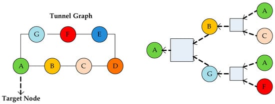
Figure 1.
Framework tunnel graph and node A’s computational diagram.
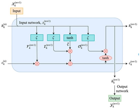
Figure 2.
Framework of LSTM.
The graph convolution formula is as follows:
where represents the learnable neural layer, and . where denotes the feature matrix (traffic flow) of all sites in tunnel. Here, denotes the feature dimension, represents the -th layer’s output.
The LSTM consists of three main components: the forget gate , the input gate , and output gate . In addition, there is a cell state used to store and pass information, and each component is composed of one or more fully connected layers for weighting, activation, and gating operations on the input.
The forget gate controls which information from the previous time step’s cell state needs to be retained or forgotten to avoid irrelevant information interfering with the current state. The updated formula for the forget gate is as follows:
The input gate is responsible for controlling the update of the cell state by the current input , determining which information needs to be added to the cell state . The sigmoid layer determines which values need to be updated, and the tanh layer creates a new candidate value vector and generates candidate memory. The state update rule for the input gate is:
The output gate is responsible for calculating the output at the current time step based on the input and memory cell state , which can be passed to the next LSTM unit or used as the final output. The state update rule of the output gate is:
The above formula shows the LSTM cell state update process, where denotes the sigmoid function; represents the candidate cell information; , , , and represent the weight coefficient matrices in the LSTM cell state update process; and , , and represent the bias matrices in the state update process.
2.3. Analysis of Output Variables
In this paper, we constructed both a BP neural network and a random forest model to predict the traffic flow status and accident duration when accidents occur. Therefore, the output variables are:
- Traffic flow status when accidents occur: According to the special situation record data of Ying Tian Avenue Tunnel, the traffic flow status when accidents occur is divided into two categories: normal traffic flow takes 0 and traffic congestion caused by accidents takes 1.
- Accident duration: In minutes, based on the special situation record data of Ying Tian Avenue Tunnel, the accident duration ranges from 0 to 38 min.
2.4. Traffic Condition Prediction Model
During traffic accidents, the traffic flow status is one of the most basic pieces of information to investigate and one of the most intuitive manifestations after the accident. The traffic flow status can reflect the road capacity to a certain extent after the accident, but it is not exactly the same as the road capacity, and there is a certain correlation between the two. Therefore, predicting the traffic flow status is the basis for predicting the duration of the highway tunnel and analyzing the traffic capacity. Predicting the traffic flow status of highway tunnel traffic takes it as the dependent variable, studies its relationship with each independent variable, and predicts the possible traffic flow status in the event of an accident through the independent variable to facilitate the prediction and handling of other situations that may occur during the accident.
2.4.1. Correlation Analysis
Undoubtedly, having a large dataset is a bonus for predicting accident targets. However, it also brings up the issue of variable selection. This includes a large number of variables directly in classification or regression models that may lead to overfitting, which in turn may affect the interpretation of the relationships between variables and, more importantly, the use of the model in the prediction phase. Therefore, it is important to analyze our data to determine which variables are the main influencing factors of the dependent variable. In order to achieve this, Pearson correlation analysis was used in this paper to study the correlation between independent and dependent variables, with the specific formula as follows [27]:
The correlation coefficient of independent variable X and dependent variable Y, is the covariance between variables X and Y, and is the variance of the variable.
2.4.2. Model for Predicting Traffic Conditions
Based on the variable screening results described above, this article predicts the traffic conditions and duration of highway tunnel accidents using both the BP neural network model and the random forest model. A total of 150 traffic accidents were randomly divided into 120 as the training set (train label) and 30 as the testing set (test label). For predicting tunnel traffic conditions, which is a classification problem, the model’s performance is evaluated by its prediction accuracy. For predicting accident duration, which is a regression problem, the evaluation is based on the root mean square error between predicted values and actual values. The formulas for calculating accuracy and root mean square error are as follows:
In the formula, represents the accuracy of the model prediction, is the number of accurate predictions, is the number of data points in the training set during training, or the number of data points in the testing set during testing.
The denotes the number of sample, denotes the ground truth, represents the predicting value.
2.4.3. BP Neural Network
The BP neural network is a type of multi-layer feedforward neural network proposed by Rumelhart in 1986 and is one of the most widely used neural networks. The BP neural network consists of an input layer, a hidden layer, and an output layer, each layer containing several neurons, with each neuron receiving signals only from the neurons in the previous layer and having no connection with the neurons in the same layer. In 1989, Robert Hecht-Nielsen proved the universal approximation theorem of the BP neural network, which states that any continuous function on a closed interval can be approximated by a BP network with only one hidden layer. Therefore, a three-layer (input layer, hidden layer, and output layer) BP neural network can complete the mapping from any dimension to any other dimension. The following Figure 3 shows a typical 3-layer BP neural network model.
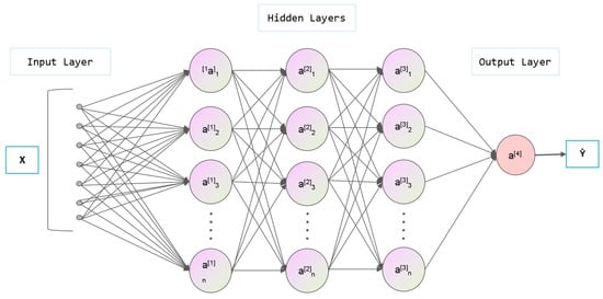
Figure 3.
The framework of BP neural network.
- Forward propagation process
Assuming that denotes input neurons, represents hidden neurons, represent output neurons, for a certain input , the output of the network is , the output of node is , and is the connection weight.
The input of hidden node :
The output of hidden layer node :
The input of output layer node :
The output of node :
The represents the activate function and, in this paper, we use sigmoid function as follows:
After the above forward propagation process, the BP neural network completes the approximate mapping from an n-dimensional space to an m-dimensional space.
- Backpropagation process
The essence of the backpropagation process is the search for weight vectors, which requires continuously iterating to minimize the error function. When the difference between the actual output of the network and the expected output does not meet the expectations, an error signal is generated and propagated from the output end to the input end. During the propagation process, the network dynamically adjusts the network weights based on the error signal feedback to continuously reduce the difference between the actual and expected output values.
Assuming that number of samples are p, after the p sample is input to the network, the output is obtained, and the expected output is . If the square error function is used, then the error of the p sample is :
The global error of the samples:
- Advantages of BP neural networks
As an artificial intelligence model, one of the most significant features that distinguishes BP neural networks from statistical regression models is that it does not require any assumptions. It can map the relationship between n-dimensional input variables and m-dimensional output variables as long as there are enough samples. The mathematical theory has proven that BP networks can approximate any complex function through the combination of simple nonlinear processing units. When the BP network encounters test samples that were not present in the training samples, it can still make correct predictions, and this ability is known as the model’s generalization ability. The BP neural network has strong generalization ability and therefore has high practical value. In some cases, there may be errors in traffic accident samples due to the large sample size, making it difficult to avoid such errors in the data. However, because BP neural networks are less affected by the global mapping capability of the network when only a few local neurons are damaged, they can achieve accurate predictions even with a small amount of error in traffic accident data.
2.4.4. Random Forest Model
Random Forest is a type of machine learning model that utilizes the concept of a collection of decision trees. Figure 4 shows the framework of the random forest model. Each tree in the random forest is built using a randomly sampled subset of data and a randomly selected subset of features. The prediction of the random forest model is based on the average prediction of all individual trees in the ensemble. Random Forest is popular due to its ability to handle high-dimensional data, detect complex interactions between variables, and avoid overfitting.
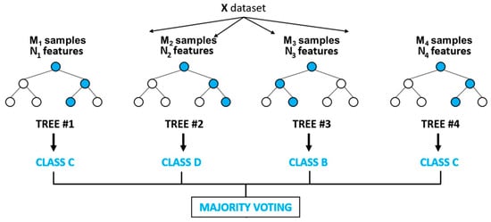
Figure 4.
Framework of random forest.
First, bootstrap sampling is used to randomly select multiple subsets of samples with replacements from the original training set; then, for each sample subset, a decision tree is generated by randomly selecting some features, and a random forest classifier is constructed. In the constructed random forest classifier, each decision tree is a learner. Next, the test set is input to the random forest model, and for each sample, each decision tree will generate its corresponding classification result. Finally, the prediction results of the base classifiers are summarized, and the final classification result of each sample is determined by voting. In summary, building a random forest model requires steps, such as data preprocessing, random sampling of data, constructing decision trees, prediction, parameter tuning, and model evaluation. Choosing appropriate parameters and variables will help improve the accuracy and predictive ability of the model.
Currently, the most widely used decision tree generation algorithms are ID3, C4.5, and CART. In these algorithms, the node split criterion in ID3 and C4.5 is calculated according to information gain, while in CART, it is calculated according to Gini impurity.
In this article, the decision tree uses the C4.5 algorithm. Decision trees generated using the ID3 algorithm are prone to the phenomenon of local optimum solutions. Therefore, Quinlan subsequently improved the node split selection criterion in the ID3 algorithm and proposed the C4.5 algorithm. The C4.5 algorithm uses information gain ratio as the feature selection criterion, and the calculation method of the information gain ratio is as follows:
where is the weight assigned to the node based on the number of samples. Compared to the ID3 algorithm, the C4.5 algorithm has improved classification accuracy.
3. Results
3.1. Pearson Correlation Analysis
After the Pearson correlation analysis, the correlation coefficients of each independent variable to the dependent variable are shown in the Figure 5 below (target is the dependent variable, taking the tunnel traffic conditions as an example). It can be seen from the figure that the accident type V8 has a high correlation with the road traffic conditions inside the tunnel, as the single-vehicle accidents are mainly collisions with the wall and abnormal parking, while the two-vehicle accidents are mainly rear-ending collisions and rubbing. This variable is not only important for predicting road traffic conditions but also for predicting the duration of accidents. In terms of time, the accident time V0 (day or night) has the highest correlation with whether the tunnel is in a high-traffic period during accident V1. The correlation between the accident date (whether it is a holiday), season, and tunnel traffic conditions during the accident is small. In terms of space, the accident location V6 (whether it is inside the tunnel) has the greatest influence, followed by whether it is in a deceleration zone, and the tunnel length and accident section have a relatively small impact. In terms of traffic volume, the ratio of traffic volume at the time of the accident to the average traffic flow during the same period of the month V7 and the mixing rate of large vehicles V9 have a greater impact on the traffic conditions. In addition, the weather V5 also has a significant impact on the tunnel traffic conditions after the accident.
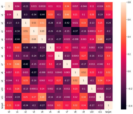
Figure 5.
Correlation heatmap between independent and dependent variables.
After analysis and comparison, the seven most relevant independent variables were selected to predict the tunnel traffic condition and accident duration during accidents. They are the involved accident types (V8), accident time (V0), accident location (V6), rate of large vehicles mixed in traffic (V9), the ratio of traffic volume during an accident to the average traffic volume in the same period of the month (V7), whether it is a traffic peak period (V1), and weather (V5) (See Figure 6).
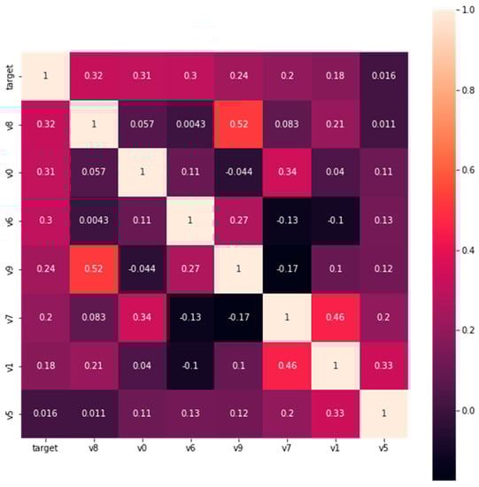
Figure 6.
Selected correlation heatmap between independent and dependent variables.
3.2. Missing Data Prediction
In the application of GCN-LSTM for missing traffic flow prediction, we treat the missing traffic flow as the value to be predicted and use the time periods with complete traffic flow records as the training set. The entire dataset is divided into an 80% training set and a 20% test set. The training and evaluation process is based on the PyTorch framework, and the model loss function adopts Mean Squared Error (MSE). The model loss reduction and prediction results are shown in Figure 7.
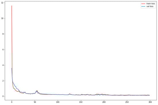
Figure 7.
Loss in train and valid datasets.
As shown in the Figure 8, the purple curve represents the actual values of the test set, and the red curve represents the predicted values of the model. Whether it is during peak hours or off-peak periods, the GCN-LSTM model is able to predict the missing traffic volume values accurately. Therefore, the predicted results can be used to calculate the input variable “the ratio of traffic volume at the time of the accident to the average traffic flow during the same period of the month”, which can then be used to predict the traffic conditions and the duration of the accident.
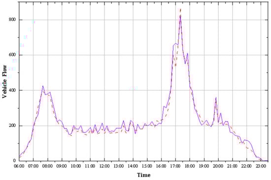
Figure 8.
Test dataset predictions.
3.3. Tunnel Traffic Condition Prediction
Based on the variable selection results in Section 3.1, after normalization, the variables were input into both the BP neural network and random forest model for prediction. This paper uses a linear function transformation method to convert the input data into data between 0 and 1:
where is the normalized value of the j-th sample of the i-th variable, is the actual input value of the j-th sample of the i-th variable, is the maximum value of the variable samples, and is the minimum value of the variable samples.
- BP neural network
The BP neural network model in this paper was trained based on the PyTorch deep learning framework. The training process was set with a learning rate of 1 × 10⁻³, 3 hidden layers with 12 neurons in each. The loss function during the training phase was calculated using the accuracy formula. The activation functions used were the sigmoid and SoftMax functions, and the optimizer used was Adam. The training was carried out for 30,000 iterations (epochs). The model was run five times, and the results are shown in Table 6:
Table 6.
Accuracy of BP neural network.
As can be seen from the table, the accuracy of the BP neural network model for predicting traffic flow conditions is about 82%, and the prediction results are relatively accurate. The time for completing one model training is around 10 s, which is short. Therefore, the BP neural network model has good robustness for predicting traffic flow conditions when accidents occur.
- Random-forest model
The random forest model has good predictive performance, so in the actual operation of the model, in order to save time and improve efficiency, it is often not necessary to adjust all parameters to ensure high model accuracy. To improve the running efficiency, this article mainly selects two main parameters for adjustment, namely, the number of decision trees (n_estimators) and the maximum depth of decision trees (max_depth). The parameter adjustment mainly uses the GridSearchCV class in the sklearn.model_selection library in Python, that is, grid search. The main function of this class is to automatically adjust the parameters. As long as the range of parameter values is given, the parameter values corresponding to the optimal result can be obtained. At the same time, this class can also perform cross-validation for each parameter combination. Through grid search and cross-validation, the optimal values of n_estimators and max_depth of the model can be obtained. Through experiments, the optimal number of decision trees for the random forest model in this article is 200, and the optimal maximum depth of decision trees is 10. The model was run five times, and the results are shown in Table 7:
Table 7.
Accuracy of random forest.
3.4. Accidents during Time Prediction
The duration of a traffic accident refers to the total time from the occurrence of the accident to the restoration of normal traffic conditions. It includes four parts: the time of accident discovery, the time of accident response, the time of accident clearance, and the time of traffic recovery. Predicting the duration of a traffic accident can provide accurate predictions of road closure time after the occurrence of an accident, which can be provided to drivers to facilitate the cancellation or change of their travel routes and enable accident handlers to effectively manage the accident scene with ease. For predicting the duration of a traffic accident, the model inputs and parameter selection are the same as those of the method for predicting the shape of the accident presented earlier. The prediction results of the two methods are presented below.
Through experimental data, the stochastic forest and BP neural network models were 75% and 60% accurate, respectively, in predicting the duration of accidents when the absolute error was less than 25 min. The results of accident duration prediction by the BP neural network model are shown in Figure 9 below, where the blue curve represents the actual accident duration of the test set, the red curve represents the prediction result of the random forest model, and the green curve represents the prediction result of the BP neural network. As shown in the figure, the trend of the accident duration predicted by the BP neural network is generally consistent with the actual value, but due to the large discreteness of the actual values, the BP neural network has reduced the discreteness of the predicted values to avoid greater errors. Therefore, the predicted values mostly fall between 3 min and 20 min, and the accuracy of predicting traffic accidents with a duration between 6 min and 20 min is relatively high. However, due to the strong discreteness of accident duration, the predictive ability of the model is poor. On the other hand, the random forest model shows a trend of accident duration that is generally consistent with the actual value and has a better-fitting effect. As shown in the figure, the predicted values mostly fall between 5 min and 25 min, and the accuracy of predicting traffic accidents with duration between 5 min and 30 min is relatively high. Therefore, the random forest model has a better fitting effect than the BP neural network in predicting accident duration.
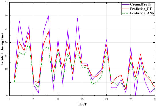
Figure 9.
Comparison of Test Set Predictions.
To improve the interpretability of model predictions, we used Shape (Shapley Addictive Explanations) for better predictive stochastic forest models to analyze the relative impact of independent variables on the target variable, i.e., the duration of an event. We used the Summary Plot method to map the Shape value of each feature for each sample, explaining which features are most important and their impact on the dataset. The position on the y-axis is determined by characteristics and the position on the x-axis is determined by each Shapley value. Colors represent eigenvalues (red is high, blue is low), and colors allow us to match how changes in eigenvalues affect changes in risk. Overlapping points wobble on the y-axis, so we can understand the Shapley value distribution of each feature, and these features are sequenced according to their importance. As shown in Figure 10, the order of importance of the feature variables is as follows: involved accident types (V8), accident location (V6), accident time (V0), the ratio of traffic volume during accident to the average traffic volume in the same period of the month (V7), and weather (V5), whether it is a traffic peak period (V1), rate of large vehicles mixed in traffic (V9).
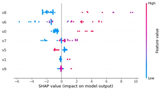
Figure 10.
SHAP value distribution.
4. Discussion
In this paper, we review the relevant literature on road traffic crashes combined with machine learning and summarizes and discusses various factors affecting the safety of road tunnels, including tunnel geometry, road surface condition, and traffic condition. The study also analyzed 38,786 traffic flow data and 200 accident data obtained from the Yingtian Tunnel in Nanjing, China, and was conducted on the same day. To account for missing traffic data, we combined the actual location of the tunnel flow logging equipment with the spatiotemporal relevance of the traffic data and designed a deep learning framework based on GCN-LSTM to predict the missing traffic flow values. We believe that our approach is more compelling and generalizable than traditional methods of using mean filling-in or direct deletion. This was followed by a combination of previous studies and correlation analysis to investigate factors affecting tunnel capacity and accident duration and visualization of the results using heat maps. Our study shows that seven independent variables—the type of accident, the time of the accident, the location of the accident, the proportion of heavy vehicles, the ratio of traffic during the accident to average traffic during the same month, if it was a peak-hour cycle, and weather—have a significant impact on tunnel capacity and accident duration, whereas other factors are insignificant. Thus, we confirm these seven variables as inputs to subsequent prediction models.
Based on the above work, we built a prediction model of highway tunnel traffic accident severity using random forest and reverse propagation neural network, with time, tunnel environment, and traffic dynamics as input variables and tunnel traffic condition and accident duration as output variables. The results of this study showed that BP neural network and random forest model both performed well in predicting traffic conditions after a tunnel accident. Both models were run five times under the same experimental setting and hyperparameters. The BP neural network had an average prediction accuracy of 82.94%, standard deviation of 1.31; and the random forest model had an average prediction accuracy of 83.39% and a standard deviation of 0.81. The prediction accuracies of the stochastic forest model and the BP neural network are 75% and 60% in terms of accident duration, respectively, when we set the absolute error to less than 25 min.
5. Conclusions
In this research, we primarily investigate the prediction of traffic accidents in long tunnels in cities. We also design a deep learning-based framework, namely, GCN-LSTM, to predict and fill in the missing values of the input variables, in addition to analyzing the traffic accidents themselves. This method can be applied to traffic research in other scenarios in the future, in particular missing data on traffic flows in large road networks. Random forest and BP neural networks are used in studies of traffic accidents and accident durations for two reasons. First, a large of prior research has confirmed that both models perform well in crash analysis and forecasting in other scenarios. Second, both of these models have better landing prospects than other more complex deep learning frameworks, and they have better accuracy than traditional models based on statistics. Our work may provide guidance to transportation operators in formulating more rational policies during special hours and provide a relevant benchmark for the implementation of emergency relief in long-distance urban tunnels. However, it should be noted that the study only used data from 200 vehicular accidents in a tunnel in Nanjing, which could limit the representativeness of the findings. Given these limitations, we will thus focus on the following directions for future work, one of which is to continue collecting more data on traffic accidents, not only from the inside of the tunnel but also from the road network surrounding the tunnel. By improving the data, we can improve the feature extraction of the model, which will make a significant contribution to the model’s credibility and robustness. Second, we view deficits in data quality and quantity as inevitable in some scenarios, and that small-sample learning may be the key to addressing this issue.
Author Contributions
Conceptualization, Y.S. and F.W.; methodology, Y.S.; software, Y.S.; validation, Y.S. and F.W.; formal analysis, F.W.; investigation, Y.S.; resources, Y.S.; data curation, F.W.; writing—original draft preparation, F.W.; writing—review and editing, Y.S.; visualization, F.W.; supervision, C.Z.; project administration, C.Z.; funding acquisition, C.Z. All authors have read and agreed to the published version of the manuscript.
Funding
This work was supported in part by the Jiangsu Transportation Science and Technology Project (2021G09).
Institutional Review Board Statement
Not applicable.
Informed Consent Statement
Not applicable.
Data Availability Statement
On behalf of all the authors, the corresponding author states that our data are available upon reasonable request.
Acknowledgments
We acknowledge the funding support from the Jiangsu Transportation Science and Technology Project Fund and the contribution of Nanjing Communication Group.
Conflicts of Interest
The authors declare no conflict of interest.
References
- Skabardonis, A.; Varaiya, P.; Petty, K.F. Measuring Recurrent and Nonrecurrent Traffic Congestion. Transp. Res. Rec. J. Transp. Res. Board 2003, 1856, 118–124. [Google Scholar] [CrossRef]
- Hamad, K.; Al-Ruzouq, R.; Zeiada, W.; Abu Dabous, S.; Khalil, M.A. Predicting incident duration using random forests. Transp. A Transp. Sci. 2020, 16, 1269–1293. [Google Scholar] [CrossRef]
- Hojati, A.T.; Ferreira, L.; Washington, S.; Charles, P.; Shobeirinejad, A. Modelling the impact of traffic incidents on travel time reliability. Transp. Res. Part C Emerg. Technol. 2016, 65, 49–60. [Google Scholar] [CrossRef]
- Li, J.; Li, J. Dynamic Comprehensive Evaluation of Transport Environment Based on Support Vector Machine. In Proceedings of the International Conference on Transportation Engineering, Chengdu, China, 22–24 July 2007. [Google Scholar] [CrossRef]
- Huo, Y.; Chen, J.; Zhang, Z. Traffic Congestion Pricing Based on Decision Tree. In Proceedings of the International Conference on Transportation Engineering, Chengdu, China, 25–27 July 2009. [Google Scholar] [CrossRef]
- Dogru, N.; Subasi, A. Traffic accident detection using random forest classifier. In Proceedings of the 2018 15th Learning and Technology Conference (L&T), Jeddah, Saudi Arabia, 25–26 February 2018; pp. 40–45. [Google Scholar] [CrossRef]
- Wang, F.; Wang, J.; Zhang, X.; Gu, D.; Yang, Y.; Zhu, H. Analysis of the Causes of Traffic Accidents and Identification of Accident-Prone Points in Long Downhill Tunnel of Mountain Expressways Based on Data Mining. Sustainability 2022, 14, 8460. [Google Scholar] [CrossRef]
- Lu, L.; Lu, J.; Xing, Y.; Wang, C.; Pan, F. Statistical Analysis of Traffic Accidents in Shanghai River Crossing Tunnels and Safety Countermeasures. Discret. Dyn. Nat. Soc. 2014, 2014, 824360. [Google Scholar] [CrossRef]
- Al-Ghamdi, A.S. Using logistic regression to estimate the influence of accident factors on accident severity. Accid. Anal. Prev. 2002, 34, 729–741. [Google Scholar] [CrossRef] [PubMed]
- Pande, A.; Abdel-Aty, M. Market basket analysis of crash data from large jurisdictions and its potential as a decision support tool. Saf. Sci. 2009, 47, 145–154. [Google Scholar] [CrossRef]
- Bezuglov, A.; Comert, G. Short-term freeway traffic parameter prediction: Application of grey system theory models. Expert Syst. Appl. 2016, 62, 284–292. [Google Scholar] [CrossRef]
- Jurewicz, C.; Excel, R. Application of a Crash-predictive Risk Assessment Model to Prioritise Road Safety Investment in Australia. Transp. Res. Procedia 2016, 14, 2101–2110. [Google Scholar] [CrossRef]
- Karimnezhad, A.; Moradi, F. Road accident data analysis using Bayesian networks. Transp. Lett. 2016, 9, 12–19. [Google Scholar] [CrossRef]
- Sattar, K.; Oughali, F.C.; Assi, K.; Ratrout, N.; Jamal, A.; Rahman, S.M. Transparent deep machine learning framework for predicting traffic crash severity. Neural Comput. Appl. 2022, 35, 1535–1547. [Google Scholar] [CrossRef]
- Lee, Y.; Wei, C.-H. A Computerized Feature Selection Method Using Genetic Algorithms to Forecast Freeway Accident Duration Times. Comput. Civ. Infrastruct. Eng. 2010, 25, 132–148. [Google Scholar] [CrossRef]
- Valenti, G.; Lelli, M.; Cucina, D. A comparative study of models for the incident duration prediction. Eur. Transp. Res. Rev. 2010, 2, 103–111. [Google Scholar] [CrossRef]
- Tang, J.; Liang, J.; Han, C.; Li, Z.; Huang, H. Crash injury severity analysis using a two-layer Stacking framework. Accid. Anal. Prev. 2018, 122, 226–238. [Google Scholar] [CrossRef] [PubMed]
- Basso, F.; Basso, L.J.; Bravo, F.; Pezoa, R. Real-time crash prediction in an urban expressway using disaggregated data. Transp. Res. Part C Emerg. Technol. 2018, 86, 202–219. [Google Scholar] [CrossRef]
- Ji, Y. Prediction of freeway incident duration based on the multi-model fusion algorithm. In Proceedings of the 2011 International Conference on Remote Sensing, Environment and Transportation Engineering, Nanjing, China, 24–26 June 2011; pp. 3327–3329. [Google Scholar] [CrossRef]
- Lin, L.; Wang, Q.; Sadek, A.W. A combined M5P tree and hazard-based duration model for predicting urban freeway traffic accident durations. Accid. Anal. Prev. 2016, 91, 114–126. [Google Scholar] [CrossRef] [PubMed]
- Jamal, A.; Zahid, M.; Rahman, M.T.; Al-Ahmadi, H.M.; Almoshaogeh, M.; Farooq, D.; Ahmad, M. Injury severity prediction of traffic crashes with ensemble machine learning techniques: A comparative study. Int. J. Inj. Control. Saf. Promot. 2021, 28, 408–427. [Google Scholar] [CrossRef] [PubMed]
- van Lint, J.W.C.; Hoogendoorn, S.P.; van Zuylen, H. Accurate freeway travel time prediction with state-space neural networks under missing data. Transp. Res. Part C Emerg. Technol. 2005, 13, 347–369. [Google Scholar] [CrossRef]
- Li, L.; Su, X.; Zhang, Y.; Hu, J.; Li, Z. Traffic prediction, data compression, abnormal data detection and missing data imputation: An integrated study based on the decomposition of traffic time series. In Proceedings of the 17th International IEEE Conference on Intelligent Transportation Systems (ITSC), Qingdao, China, 8–11 October 2014; pp. 282–289. [Google Scholar] [CrossRef]
- Zhang, Z.; Liu, Z.; Zhou, Q.; Qu, Y. Cross Message Passing Graph Neural Network. In Proceedings of the 2020 International Joint Conference on Neural Networks (IJCNN), Glasgow, UK, 19–24 July 2020; pp. 1–7. [Google Scholar] [CrossRef]
- Agafonov, A. Traffic Flow Prediction Using Graph Convolution Neural Networks. In Proceedings of the 2020 10th International Conference on Information Science and Technology (ICIST), Bath, London, and Plymouth, UK, 9–15 September 2020; pp. 91–95. [Google Scholar] [CrossRef]
- Duan, Y.; Lv, Y.; Wang, F.-Y. Travel time prediction with LSTM neural network. In Proceedings of the 2016 IEEE 19th International Conference on Intelligent Transportation Systems (ITSC), Rio de Janeiro, Brazil, 1–4 November 2016; pp. 1053–1058. [Google Scholar]
- Djordjević, B.; Mane, A.S.; Krmac, E. Analysis of dependency and importance of key indicators for railway sustainability monitoring: A new integrated approach with DEA and Pearson correlation. Res. Transp. Bus. Manag. 2021, 41, 100650. [Google Scholar] [CrossRef]


Disclaimer/Publisher’s Note: The statements, opinions and data contained in all publications are solely those of the individual author(s) and contributor(s) and not of MDPI and/or the editor(s). MDPI and/or the editor(s) disclaim responsibility for any injury to people or property resulting from any ideas, methods, instructions or products referred to in the content. |
© 2023 by the authors. Licensee MDPI, Basel, Switzerland. This article is an open access article distributed under the terms and conditions of the Creative Commons Attribution (CC BY) license (https://creativecommons.org/licenses/by/4.0/).