Abstract
Defective droppers pose a significant threat to the performance of the contact between the train pantograph and railway catenary. In this paper, the impact of damaged droppers on the performance of pantograph–catenary interaction behaviour is analysed, and the impact of varying degrees of damage to each dropper is labelled. To improve the classification accuracy when both the damage degree and position are considered, a model integrating multiple 1D CNNs is proposed. Approaches including randomly searching the optimal hyper-parameters and K-fold cross-validation are used to prevent overfitting and to ensure model performance regardless of the training data subset selected. Compared with a conventional 1D CNN, the classification performance of the integrated method is demonstrated using the metrics accuracy, F1-score, precision and recall. It is concluded that, through the use of the integrated 1D CNN, damaged droppers can be detected and localised based on the pantograph–catenary contact force. Hence, intelligent catenary inspection can be enhanced.
1. Introduction
Railway electrification has been undertaken since the late 19th century [1] and the scale of the electrified line has been increased worldwide by more than fifty percent over the last two decades [2] due to its advantage in energy efficiency. As wear and tear accumulate in daily operations, the malfunction and wearing out of physical components in the overhead line (i.e., railway catenary) system, one of the current supply forms, is unavoidable. Defects of the catenary droppers, support and contact wire irregularity have been identified as posing substantial threats to current collection [3,4,5,6,7,8]. In order to reduce the risk from a defective catenary, its health condition is routinely inspected by railway operators that traditionally rely on skilled engineers [9]. To improve the efficiency of maintenance, a number of catenary inspection studies have been conducted in recent years through image processing based on on-vehicle-roof cameras [10,11,12,13,14,15,16], which have shown satisfactory effectiveness.
Besides utilising the image signal to monitor catenary health, the contact behaviour of the pantograph–catenary interaction is also potentially effective [17,18,19,20], as it can offer a straightforward insight into the impact on energy transmission quality. In analysing contact behaviour between the pantograph and catenary, the contact force is one of the essential indicators [9]. The pantograph–catenary contact force signal is usually measured by placing load cells between the collector and its suspension or by fitting fibre-optic sensors under the carbon strip [9]. Some prototypes have been tested on main lines [21,22,23,24,25]. Alternatively, suitable numerical models of the pantograph–catenary system can also be applied to generate the contact force for signal processing when a series of defective cases are considered [7,17,18].
In recent years, finite element (FE)-based catenary models have dominated research focusing on pantograph–catenary dynamics [9,26]. The method approximates the catenary by discretising the system into smaller physics-based elements, which provides excellent accuracy and consistency [21,24,26,27]. When contact force is the main interest, the pantograph is commonly modelled by a lumped-mass model for simulations [9,26]. However, to ensure the veracity of the pantograph–catenary models, the simulation framework is required to be validated by the simulation standard EN50318 [28].
Either from experimental data or simulation results, dropper defects have been identified as being critical to the pantograph–catenary interaction performance [3,5,16,20]. The contact force signal is effective for finding fault information through static-based or signal-processing techniques. For example, in [7], contact force signals with defective droppers were obtained from an FE catenary model. The results were then subjected to time and frequency analysis techniques. In the time domain, the variance of different faults was obviously found when investigating peaks at some specific locations (local peaks). This study identified the feature of defective droppers, but there are few studies focused on damage classification. Additionally, the data used in [7] do not contain any noise, so they do not reflect real-world influences. Hence, further research on the detection and localisation of defective droppers is worthy of investigation.
A convolutional neural network (CNN) as a standard deep learning technique has been effectively used in many research domains (fault classification, linear regression, speech recognition, etc.) [29,30,31,32]. Generally, a CNN consists of CNN layers and multilayer perceptron (MLP) layers [33]. The CNN layer is used to process the data and extract the feature, and the MLP layers can perform classification according to the identified features. Considering the application of CNN for the inspection of the catenary system, some studies focusing on the image (2-dimensional signal) have been carried out [10,11,12,13,14,15,16]. Among them, Ref. [16] tackled the classification problem of defective droppers, where photos of droppers were captured by roof-mounted cameras on vehicles. According to the CNN method, the features of healthy and defective droppers have been identified and classified. However, as mentioned in this paper, it is difficult to classify damage that is not visually obvious.
An alternative to the image-based approach is to make use of contact force. Contact force has the advantage that it can reflect the pantograph–catenary contact quality straightforwardly, no matter the shape of the dropper. However, because the contact force is a 1-dimensional signal, the previously mentioned techniques cannot be applied directly. Hence, the related 1D CNN approaches should be explored. The effectiveness of 1D CNN models has been demonstrated and they have been widely used across a range of applications [34].
However, considering the problem of using 1D CNN to detect and localise the fault simultaneously, it has been found that a conventional machine learning technique is not efficient [35]. Hence, it is suggested to integrate separate 1D CNNs for fault detection and localisation tasks.
Considering the above discussion, the objective of this paper is to detect and localise defective droppers in a railway catenary through the pantograph–catenary contact force. The FE catenary model will be developed and used to generate the required contact force data, with and without faults. The impact of the damage to each dropper on the contact behaviour can be analysed and categorised. Noise will be added to the data to imitate real-world disturbance. Once the data are available, two 1D CNNs are integrated (integrated 1D CNN) to detect the degree of damage and location of the defective dropper as independent tasks. The main contributions of this paper are as follows.
- (a)
- The impact of dropper defects on railway pantograph–catenary interaction is analysed, and the impact of varying degrees of damage to each dropper is categorised.
- (b)
- An integrated 1D CNN is used to improve classification performance compared with a conventional 1D CNN. Approaches including randomly searching the optimal hyper-parameters and K-fold cross-validation are considered to prevent overfitting and ensure model performance regardless of the training data subset selected.
- (c)
- The ability of the 1D CNN-based method to evaluate the degree of damage to catenary droppers and locate the position of defective droppers within a catenary system is demonstrated.
2. Pantograph–Catenary System Modelling
The contact and messenger wires in the catenary system are modelled by a 2D Euler–Bernoulli beam whose vertical dynamic behaviour follows:
where , , , , , , , , and denote the density of the wire, the cross-sectional area of the wire, the vertical deflection of the wire, the elapsed time, the tensile force of the wire, the Young’s modulus of the wire, the second moment of area of the wire, the horizontal location of the measured point, the damping coefficient, and the external force, respectively.
To represent the kinetics by means of FEs, the system is discretised into small FEs, and the dynamic behaviour of each element node can be approximately a function of the states of itself and its adjacent ones (i.e., deflection and slope). Hence, the system dynamics can be assembled and obtained, as in Equation (2).
where is the states of nodes; , and are the assembled mass, stiffness, and damping, respectively (the damping coefficient is assumed to be proportional to mass and stiffness); and denotes the external force on the nodes including the pantograph–catenary contact force and those exerted by other catenary components (i.e., dropper, steady arm and messenger wire suspension).
The dropper is represented by a spring model with slackening as in Equation (3), whose elasticity changes with the spring state. In this study, as the defective dropper is of concern, the elasticity varies, ranging from 100% to 0% of the nominal value to represent dropper damage conditions. It should be noted that the initial condition of the catenary system is affected by the defective dropper, which will be incorporated in the model.
The material properties and structural information on the catenary model are taken from [28] and an existing academic benchmark [26]. Besides that, a validated three-mass lumped-mass pantograph model [26] is used for the simulations. To generate the pantograph–catenary contact force, a virtual spring of 50,000 N/m is placed between the pantograph head and the contact wire [26,28]. The above pantograph–catenary model is depicted in Figure 1 and the parameters are summarised in Table 1. The Newmark-beta method with the rule of average constant acceleration is applied for time integration in simulations. The model validation will be given in the next section.
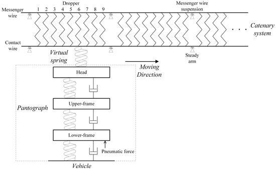
Figure 1.
FE catenary with pantograph mode.

Table 1.
Parameters of the pantograph–catenary model.
3. Simulations and Damage Classification
3.1. Static Analysis
Based on the above numerical model, the simulation for a healthy catenary and one with a defective dropper can be conducted. For the sake of brevity, only the fifth dropper’s defect is presented to demonstrate the impact of the damage.
Figure 2 shows the dropper impact on the contact wire static state that consists of the vertical displacement and the static stiffness over a span. It shows that the impact of the fifth dropper’s defect increases non-linearly with the degree of damage. When the dropper nearly loses its elasticity or has done so already, the difference from the nominal condition is considerable.
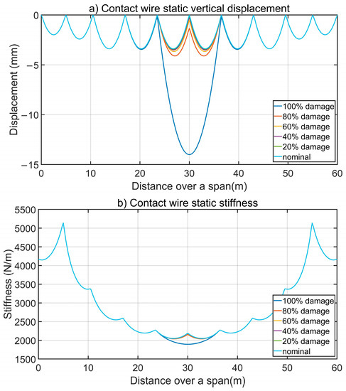
Figure 2.
Static impact on the contact wire state (a) the displacement (b) the stiffness.
3.2. Model Validation and Dynamic Simulation
To evaluate the impact on dynamic performance, the catenary is integrated with the pantograph at a speed of 250 km/h. A 10-span catenary with nominal dropper conditions is simulated to validate against [28], which is presented in Table 2. The simulation framework has also been validated in [36] but, for the sake of brevity, the details are not presented here.
Table 2.
Model validation at 250 km/h.
The impact of the fifth dropper’s damage on the contact force performance is presented in Figure 3. It can be seen that if the damage is minor, the difference in contact force can be negligible. On the contrary, if the fifth dropper fully malfunctions, its impact on force can propagate to the whole span and distort contact behaviour.
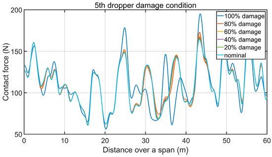
Figure 3.
Dynamic impact on contact force.
3.3. Dropper Damage Categorisation
Dropper damage is expected to be categorised and labelled for further classification. It was found in [7] that the impact of defective droppers on the quality of the contact force varies significantly across different positions. Therefore, instead of using the damage degree, the impact level on the contact force will be used for dropper condition categorisation, which can intuitively represent the impact of defective droppers on pantograph–catenary dynamics.
To quantify the impact, three key indicators of the contact force (i.e., standard deviation (std) maximum (max) and minimum (min)) are considered. They reflect the degree of mechanical wear, possibility of contact loss and contact robustness. The impact index, introduced in Equation (4), quantifies the impact of defective droppers on the contact quality. It finds the greatest deterioration in the force standard deviation, maximum, and minimum by comparing the contact force signal of the damaged catenary () with the nominal result ().
Figure 4 shows the impact index of each dropper’s defect with damage degree ranging from 100% to 0%. It is clear that each dropper’s damage has a distinctive impact on the contact performance. Regarding the index, the damage degree of each dropper is categorised into two risk categories, low risk () and high risk (). Once a damage degree is labelled, a worse degree will not be categorised as healthier than that for conservatism. The damage categorisation is summarised in Table 3. For example, if the damage of the fifth dropper is more than 27% of the nominal value, the condition will be labelled as low risk and if it is more than 62.5%, it will be labelled as high risk.
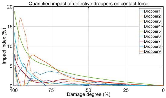
Figure 4.
Quantified impact of defective droppers on pantograph–catenary dynamic behaviour.
Table 3.
Dropper damage categorisation (D = dropper no.).
Moreover, Gaussian white noise filtered up to 20 Hz (the interested frequency range associated with the contact force) will be added to include the measurement error. According to the requirement for the measurements of the pantograph–catenary dynamic interaction, the maximum error of the measurement system should be less than 10% of the measured value [37]. After adding noise into the raw contact force result, the maximum error of all data is 8.88% at 20 dB noise power whereas it is 16.49% at 25 dB. Therefore, a noise power of no more than 25 dB is worthwhile to be considered.
4. Fault Classification through CNNs
This section introduces the process of training and validating the integrated 1D CNN model. Firstly, the method of integrating the multiple 1D CNNs including Sub-model 1 and Sub-model 2 is given. Secondly, the preparation of training and validating datasets is discussed. In order to ensure the performance of the integrated CNN model regardless of the training data subset selected, an application based on K-fold cross-validation is considered. Thirdly, a tuning technique is introduced to search for the optimal hyper-parameters of the sub-models. Finally, the evaluating metrics are explored to measure the performance of the integrated 1D CNN model.
4.1. Structure of the Integrated 1D CNN Method
In 1D CNN, the forward propagation (FP) from the convolution layer (output) to the l layer (input) is expressed as Equation (5), where is a neuron of the input layer; is the scalar bias of the kth neuron of the lth input layer; is the ith neuron from the output layer; and is the kernel from the ith neuron of the )th output layer to the kth neuron of the lth input layer.
The neuron of intermediate output is defined as , which can be obtained from input . It can be presented as Equation (6), where is a neuron of the output layer; is the down-sampling operation with the scalar factor (ss).
In this paper, a method based on integrating multiple 1D CNNs (integrated 1D CNN) is applied to classify the damage degree and the position of defective droppers as two independent tasks. The structure of the integrated 1D CNN model is shown in Figure 5. Specifically, Sub-model 1 considers the damage degree of droppers defined in Table 3. Sub-model 2 considers the location of defective droppers that comprises nine labels representing nine positions. It should be noted that when the dropper is identified as being healthy, it is not necessary to identify its position. Hence, Sub-model 2 is applied to train the part of the dataset which only contains the data labelled as ‘low risk’ and ‘high risk’ (i.e., data not labelled as “healthy”).
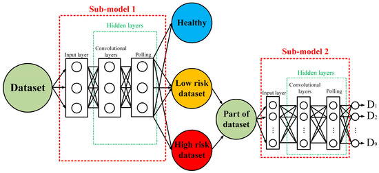
Figure 5.
Structure of the proposed integrated 1CNN model.
To integrate the two trained sub-models, a method to transmit the output result from Sub-model 1 to Sub-model 2 is proposed.
The result from Sub-model 1 is given as a set of predicted probabilities corresponding to the three damage conditions. The probabilities of ‘healthy’, ‘low risk’ and ‘high risk’ are given as P1, P2 and P3, respectively. The Pmax is the maximum value of P1, P2 and P3. If the Pmax corresponds to ‘healthy’ condition (P1), the process will stop. The predicted output of Sub-model 1 will be saved. If the Pmax belongs to ‘low risk’ or ‘high risk’ (P2 or P3), it will be fed into Sub-model 2 for further prediction. The predicted output of Sub-model 2 represents the location of the defective dropper. The testing performance of the integrated CNN model is the product of the predicted results of Sub-model 1 and Sub-model 2.
4.2. Result Analysis
(1) Dataset size and split: The data of a span-length contact force obtained from the simulation were prepared for classification. The details of the dataset are listed in Table 4.
Table 4.
Details of the dataset.
In addition, in order to demonstrate how the data are processed by the integrated 1D CNN, the data flow diagram is shown in Figure 6.
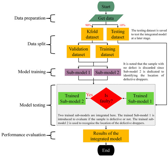
Figure 6.
Data flow diagram of the integrated CNN model.
As can be seen from Figure 6, the dataset was divided into two parts prior to the classification process. A total of 90% of the data was allocated to create a new dataset called the K-fold dataset, which was used for training and validating the integrated 1D CNNs model. For each sub-model, 75% of the corresponding K-fold dataset was utilised for training, and 25% was reserved for validation.
The remaining 10% of the data, which was not utilised in any training or validation processes, was subsequently employed to test the performance of the integrated 1D CNNs model, which consisted of the two fine-tuned sub-models.
The application of Z-score [38] was used to normalise the dataset. It is notable that the datasets for validation and testing (validation and testing dataset) were normalised based on the training dataset. Hence, during the whole process of classification, the testing dataset for the integrated 1D CNN model was not used for training and validation of the sub-models. This avoids data leakage and proves the authenticity of the validation results.
(2) K-fold cross-validation: Cross-validation measures generalised error through the existing dataset [39]. K-fold as a common cross-validation method is widely used to estimate prediction accuracy [40]. Compared with the typically practiced cross-validation method, the results from the K-fold method are closer to real performance [41].
In K-fold validation, the dataset is divided into k subsets of equal size for training and validation. In this paper, we chose 10 folds for cross-validation. Compared with other cross-validation methods, better performance with 10 folds has been proven in terms of bias and variance [42].
4.3. Hyper-Parameter Tuning Technique
As it is difficult to manually select suitable hyper-parameters for CNN models, an adaptive application [43] was used to randomly search the optimal hyper-parameters. The hyper-parameters considered including the number of filters, the number of CNN layers, weight decay, learning rate and the number of filters in the dense layers [43]. The kernel initialiser was selected between the He normal initialiser [44] and the Glorot uniform initialiser [45]. The activation function was selected between Sigmoid, Tanh and Relu. The selected ranges of these hyper-parameters are shown in Table 5. Additionally, the number of epochs for training the model was 200, and 10 trials were used for random searching of hyper-parameters. Based on the proposed method, the optimal hyper-parameters are tuned to train these two sub-models, respectively. Furthermore, selecting the optimal hyper-parameter of weight decay can effectively prevent the model from overfitting.
Table 5.
Selection range of CNN hyper-parameters.
4.4. Performance Evaluation
Accuracy, F1-score, precision and recall are four important metrics commonly used for evaluating the performance of machine-learning-based methods [46]. Accuracy is defined as the closeness of a measured value to the true value [47]. Precision and recall are metrics that evaluate the ability to retrieve data from the original dataset [48]. The F1-score is a measurement combining the precision and recall of the model to further reflect the accuracy of evaluating results [49].
Additionally, in order to demonstrate the performance of the integrated 1D CNN model, a conventional CNN with the same hyper-parameter tuning technique and K-fold validation method classifying 19 labels (2 × 9 ‘risk’ labels and 1 ‘healthy’ label) is used for comparison.
5. Results Analysis and Discussion
The dataset was used to train the integrated 1D CNN model for fault classification. The optimal hyper-parameters of the two sub-models were obtained by the tuning technique using the training and validating dataset. The details of the simulated dataset and optimal hyper-parameters of the two sub-models along with the conventional CNN model are shown in Table 6.
Table 6.
Optimal hyper-parameters of CNN model.
The results of the two sub-models and integrated 1D CNN model through evaluating four metrics (accuracy, F1-score, precision and recall) are given in Figure 7, Figure 8 and Figure 9.
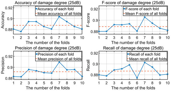
Figure 7.
Results of Sub-model 1 through four metrics (25 dB).
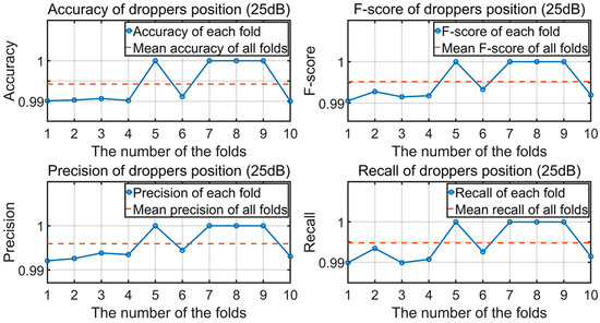
Figure 8.
Results of Sub-model 2 through four metrics (25 dB).
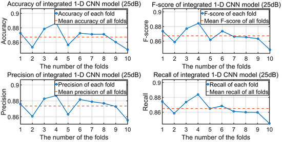
Figure 9.
Results of the integrated model through four metrics.
The performance in the four metrics is shown using the average values. Considering the metric values for all folds, the standard deviation of the results is small (all standard deviations are lower than 0.01); hence, the authenticity of the training and validating results is proven by using the K-fold cross-validation process. The average results trained by Sub-model 1, Sub-model 2 and the integrated 1D CNN model with different signal noise levels (dB) are presented in Table 7. The integrated 1D CNN model shows excellent classification performances in the four metrics (over 86%).
Table 7.
Accuracy of the first and second sub-models and the integrated 1D CNN model.
The results obtained via training of the conventional 1D CNN method, shown in Table 8, are used for comparison. These results show that both the conventional and integrated CNN-based methods are able to classify defective droppers.
Table 8.
Comparison between the conventional 1D CNN and the integrated 1D CNN model.
To compare the performance of the conventional 1D CNN and the integrated CNN, in the face of signal noise, the trend of the four metrics of the two methods with increasing noise power is shown in Figure 10.
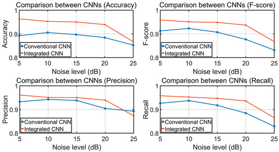
Figure 10.
Comparison of the results between integrated model and the conventional model through four metrics.
In Table 8, considering the four evaluating metrics of the integrated 1D CNN with the same noise power, the value is relatively consistent (the variance of these four values is lower than one). On the contrary, the variance of these values in the conventional 1D CNN is over 5% (at 25 dB).
In terms of performance for the four metrics, the results of the integrated 1D CNN show better performance than the conventional 1D CNN. For example, under a 20 dB noise level, the accuracy of the integrated 1D CNN model is approximately 5% higher than that of the conventional 1D CNN model, which means there will be nine fewer false/missing alarms in terms of the selected testing dataset. Similar (though slightly smaller) improvements can be seen across the three other metrics. This demonstrates that the integrated 1D CNN is more effective in classifying the fault with two categories (i.e., damage degree and location).
When the noise power increases, the values of the four performance metrics reduce. The maximum noise used in this study was 25 dB, which is more than the maximum permissible measurement error. When the noise power is 25 dB, the performance of the four values is still over 85%. This indicates that contact-force-based condition monitoring is effective in the early detection of railway catenary dropper damage.
Additionally, the computational cost is a factor of concern. In this research, the computation is based on the Google Collaboratory platform with a P100 GPU. By training the conventional 1D CNN model and the integrated 1D CNN model with their own optimal hyper-parameters, the computational costs from the two methods are compared. The computational time of the integrated 1D CNN model is increased by 4% compared with the conventional 1D CNN model.
6. Conclusions
A defective dropper in a railway catenary system is a common fault which is not easily detectable in advance using existing monitoring methods. In this paper, a computational framework was used to model the health condition of the droppers and simulate the pantograph–catenary interaction. The impact of dropper damage on the system’s dynamic behaviour was analysed and categorised in terms of contact force quality. The filtered Gaussian white noise was added to the raw data to improve the authenticity for classification.
This paper also contributes a method to classify the damage degree and the location of the defective droppers. To detect and locate damaged droppers, a method integrating multiple 1D CNN models was developed and applied. The hyper-parameter tuning technique and K-fold cross-validation were used to prevent overfitting and to ensure model performance regardless of the training data subset selected. Metrics including accuracy, F1-score, precision and recall have been considered, and the classification results show better performance of the integrated 1D CNN model than a conventional 1D CNN model. For example, under a 20 dB noise level, the accuracy of the integrated 1D CNN model was approximately 5% higher, which means there would be one in twenty fewer false alarms. It is concluded that the integrated 1D CNN method can forecast the risk of defective droppers. Regardless of the form of damage, as long as the damage affects the pantograph–catenary contact force quality, the defective dropper can be identified by the integrated 1D CNN method, which can improve the competence of intelligent condition monitoring in the railway system.
Author Contributions
This paper was written by J.Y., H.D., L.L., E.S., J.H. and R.D. The catenary simulation model was contributed by H.D. The integrated 1D CNNs model was developed by J.Y. and J.H. The results analysis was contributed by J.Y., H.D. and L.L. Project supervision was provided by E.S. and R.D. All authors have read and agreed to the published version of the manuscript.
Funding
This research was partly funded by the China Scholarship Council grant number 201908060338 and the School of Engineering at the University of Birmingham And The APC was funded by the University of Birmingham.
Data Availability Statement
All relevant data are shown in the paper or could be recreated by following the methodology in the paper.
Acknowledgments
The authors are deeply grateful to the Birmingham Centre for Railway Research and Education (BCRRE) for the resources provided.
Conflicts of Interest
The authors declare no conflict of interest.
References
- Koseki, T. Technical trends of railway traction in the world. In Proceedings of the 2010 International Power Electronics Conference-ECCE ASIA, Sapporo, Japan, 21–24 June 2010; pp. 2836–2841. [Google Scholar]
- International Union of Railway. UIC STATISTICS—Length of Electrified Lines. Available online: https://uic-stats.uic.org/ (accessed on 14 January 2023).
- Collina, A.; Fossati, F.; Papi, M.; Resta, F. Impact of overhead line irregularity on current collection and diagnostics based on the measurement of pantograph dynamics. Proc. Inst. Mech. Eng. Part F J. Rail Rapid Transit 2007, 221, 547–559. [Google Scholar] [CrossRef]
- Van, O.V.; Massat, J.-P.; Balmes, E. Waves, modes and properties with a major impact on dynamic pantograph-catenary interaction. J. Sound Vib. 2017, 402, 51–69. [Google Scholar] [CrossRef]
- Vesali, F.; Rezvani, M.A.; Molatefi, H.; Hecht, M. Static form-finding of normal and defective catenaries based on the analytical exact solution of the tensile Euler–Bernoulli beam. Proc. Inst. Mech. Eng. Part F J. Rail Rapid Transit 2019, 233, 691–700. [Google Scholar] [CrossRef]
- Song, Y.; Liu, Z.; Rønnquist, A.; Nåvik, P.; Liu, Z. Contact Wire Irregularity Stochastics and Effect on High-Speed Railway Pantograph–Catenary Interactions. IEEE Trans. Instrum. Meas. 2020, 69, 8196–8206. [Google Scholar] [CrossRef]
- Song, Y.; Liu, Z.; Lu, X. Dynamic performance of high-speed railway overhead contact line interacting with pantograph considering local dropper defect. IEEE Trans. Veh. Technol. 2020, 69, 5958–5967. [Google Scholar] [CrossRef]
- Song, Y.; Wang, H.; Liu, Z. An Investigation on the Current Collection Quality of Railway Pantograph-Catenary Systems with Contact Wire Wear Degradations. IEEE Trans. Instrum. Meas. 2021, 70, 1–11. [Google Scholar] [CrossRef]
- Bruni, S.; Bucca, G.; Carnevale, M.; Collina, A.; Facchinetti, A. Pantograph–catenary interaction: Recent achievements and future research challenges. Int. J. Rail Transp. 2018, 6, 57–82. [Google Scholar] [CrossRef]
- Chen, J.; Liu, Z.; Wang, H.; Núñez, A.; Han, Z. Automatic Defect Detection of Fasteners on the Catenary Support Device Using Deep Convolutional Neural Network. IEEE Trans. Instrum. Meas. 2017, 67, 257–269. [Google Scholar] [CrossRef]
- Zhong, J.; Liu, Z.; Han, Z.; Han, Y.; Zhang, W. A CNN-based defect inspection method for catenary split pins in high-speed railway. IEEE Trans. Instrum. Meas. 2018, 68, 2849–2860. [Google Scholar] [CrossRef]
- Lyu, Y.; Han, Z.; Zhong, J.; Li, C.; Liu, Z. A Generic Anomaly Detection of Catenary Support Components Based on Generative Adversarial Networks. IEEE Trans. Instrum. Meas. 2019, 69, 2439–2448. [Google Scholar] [CrossRef]
- Zhong, J.; Liu, Z.; Yang, C.; Wang, H.; Gao, S.; Nunez, A. Adversarial Reconstruction Based on Tighter Oriented Localization for Catenary Insulator Defect Detection in High-Speed Railways. IEEE Trans. Intell. Transp. Syst. 2020, 23, 1109–1120. [Google Scholar] [CrossRef]
- Liu, W.; Liu, Z.; Wang, H.; Han, Z. An Automated Defect Detection Approach for Catenary Rod-Insulator Textured Surfaces Using Unsupervised Learning. IEEE Trans. Instrum. Meas. 2020, 69, 8411–8423. [Google Scholar] [CrossRef]
- Liu, W.; Liu, Z.; Li, Y.; Wang, H.; Yang, C.; Wang, D.; Zhai, D. An Automatic Loose Defect Detection Method for Catenary Bracing Wire Components Using Deep Convolutional Neural Networks and Image Processing. IEEE Trans. Instrum. Meas. 2021, 70, 1–14. [Google Scholar] [CrossRef]
- Tan, P.; Li, X.; Wu, Z.; Ding, J.; Ma, J.; Chen, Y.; Fang, Y.; Ning, Y. Multialgorithm Fusion Image Processing for High Speed Railway Dropper Failure–Defect Detection. IEEE Trans. Syst. Man Cybern. Syst. 2021, 51, 4466–4478. [Google Scholar] [CrossRef]
- Song, Y.; Rønnquist, A.; Jiang, T.; Nåvik, P. Identification of short-wavelength contact wire irregularities in electrified railway pantograph–catenary system. Mech. Mach. Theory 2021, 162, 104338. [Google Scholar] [CrossRef]
- Wang, H.; Liu, Z.; Song, Y.; Lu, X.; Han, Z.; Zhang, J.; Wang, Y. Detection of Contact Wire Irregularities Using a Quadratic Time–Frequency Representation of the Pantograph–Catenary Contact Force. IEEE Trans. Meas. 2016, 65, 1385–1397. [Google Scholar] [CrossRef]
- Wang, H.; Liu, Z.; Nunez, A.; Dollevoet, R. Entropy-Based Local Irregularity Detection for High-Speed Railway Catenaries with Frequent Inspections. IEEE Trans. Instrum. Meas. 2018, 68, 3536–3547. [Google Scholar] [CrossRef]
- Zhou, N.; Yang, W.; Liu, J.; Zhang, W.; Wang, D. Investigation on monitoring system for pantograph and catenary based on condition-based recognition of pantograph. Shock. Vib. 2019, 2019, 3839191. [Google Scholar] [CrossRef]
- Collina, A.; Bruni, S. Numerical Simulation of Pantograph-Overhead Equipment Interaction. Veh. Syst. Dyn. 2002, 38, 261–291. [Google Scholar] [CrossRef]
- Paik, J.-S.; Park, C.-K.; Kim, Y.-G.; Kim, K.-H. A study on the measuring system of contact force of pantograph for the high-speed train. J. Adv. Mech. Des. Syst. Manuf. 2012, 6, 140–148. [Google Scholar] [CrossRef]
- Schröder, K.; Ecke, W.; Kautz, M.; Willett, S.; Jenzer, M.; Bosselmann, T. An approach to continuous on-site monitoring of contact forces in current collectors by a fiber optic sensing system. Opt. Lasers Eng. 2013, 51, 172–179. [Google Scholar] [CrossRef]
- Finner, L.; Poetsch, G.; Sarnes, B.; Kolbe, M. Program for catenary–pantograph analysis, PrOSA statement of methods and validation according EN 50318. Veh. Syst. Dyn. 2015, 53, 305–313. [Google Scholar] [CrossRef]
- Nåvik, P.; Rønnquist, A.; Stichel, S. Variation in predicting pantograph–catenary interaction contact forces, numerical simulations and field measurements. Veh. Syst. Dyn. 2017, 55, 1265–1282. [Google Scholar] [CrossRef]
- Bruni, S.; Ambrosio, J.; Carnicero, A.; Cho, Y.H.; Finner, L.; Ikeda, M.; Kwon, S.Y.; Massat, J.-P.; Stichel, S.; Tur, M.; et al. The results of the pantograph–catenary interaction benchmark. Veh. Syst. Dyn. 2015, 53, 412–435. [Google Scholar] [CrossRef]
- Beagles, A.; Fletcher, D.; Peffers, M.; Mak, P.; Lowe, C. Validation of a new model for railway overhead line dynamics. Proc. Inst. Civ. Eng. Transp. 2016, 169, 339–349. [Google Scholar] [CrossRef]
- BS EN 50318:2002; Railway Applications—Current Collection Systems—Validation of Simulation of the Dynamic Interaction between Pantograph and Overhead Contact Line. British Standards Institution: London, UK, 2002.
- LeCun, Y.; Boser, B.; Denker, J.; Henderson, D.; Howard, R.E.; Hubbard, W.E. Handwritten digit recognition with a back-propagation network. In Advances in Neural Information Processing Systems; Morgan Kaufmann: Burlington, MA, USA, 1989; pp. 396–404. [Google Scholar]
- Scherer, D.; Müller, A.; Behnke, S. Evaluation of pooling operations in convolutional architectures for object recognition. Int. Conf. Artif. Neural Netw. 2010, 6354, 92–101. [Google Scholar]
- Zhang, D.; Stewart, E.; Ye, J. Roller bearing degradation assessment based on a deep MLP convolution neural network considering outlier regions. IEEE Trans. Instrum. Meas. 2019, 69, 2996–3004. [Google Scholar] [CrossRef]
- Zhang, D.; Stewart, E.; Entezami, M.; Roberts, C.; Yu, D. Intelligent acoustic-based fault diagnosis of roller bearings using a deep graph convolutional network. Measurement 2020, 156, 156. [Google Scholar] [CrossRef]
- Schmidhuber, J. Deep Learning in neural networks: An overview. Neural Netw. 2015, 61, 85–117. [Google Scholar] [CrossRef]
- Kiranyaz, S.; Avci, O.; Abdeljaber, O.; Ince, T.; Gabbouj, M.; Inman, D.J. 1D convolutional neural networks and applications: A survey. Mech. Syst. Signal Process. 2021, 151, 107398. [Google Scholar] [CrossRef]
- Chen, Y.Q.; Fink, O.; Sansavini, G. Combined fault location and classification for power transmission lines fault diagnosis with integrated feature extraction. IEEE Trans. Ind. Electron. 2017, 65, 561–569. [Google Scholar] [CrossRef]
- Duan, H.; Dixon, R.; Stewart, E. A disturbance observer based lumped-mass catenary model for active pantograph design and validation. Veh. Syst. Dyn. 2022, 61, 1565–1582. [Google Scholar] [CrossRef]
- EN 50317:2012; Railway Applications—Current Collection Systems—Requirements for and Validation of Measurements of the Dynamic Interaction between Pantograph and Overhead Contact Line. British Standards Institution: London, UK, 2012.
- Cheadle, C.; Vawter, M.P.; Freed, W.J.; Becker, K.G. Analysis of microarray data using Z score transformation. J. Mol. Diagn. 2003, 5, 73–81. [Google Scholar] [CrossRef] [PubMed]
- Syed, A.R. A Review of Cross Validation and Adaptive Model Selection. Master’s Thesis, Department of Mathematics and Statistics, Georgia State University, Atlanta, GA, USA, 2011. [Google Scholar]
- Stone, M. Cross-validatory choice and assessment of statistical predictions. J. R. Stat. Soc. Ser. B 1974, 36, 111–133. [Google Scholar] [CrossRef]
- Esmaeelzadeh, S.R.; Adib, A.; Alahdin, S. Long-term streamflow forecasts by Adaptive Neuro-Fuzzy Inference System using satellite images and K-fold cross-validation (Case study: Dez, Iran). KSCE J. Civ. Eng. 2015, 19, 2298–2306. [Google Scholar] [CrossRef]
- Burman, P. A comparative study of ordinary cross-validation, v-fold cross-validation and the repeated learning-testing methods. Biometrika 1989, 76, 503–514. [Google Scholar] [CrossRef]
- Bergstra, J.; Bengio, Y. Random Search for Hyper-Parameter Optimization. J. Mach. Learn. Res. 2015, 13, 281–305. [Google Scholar]
- He, K.; Zhang, X.; Ren, S.; Sun, J. Deep residual learning for image recognition. In Proceedings of the IEEE Conference on Computer Vision and Pattern Recognition, Las Vegas, NV, USA, 26 June–1 July 2016; pp. 770–778. [Google Scholar]
- Glorot, X.; Bengio, Y. Understanding the difficulty of training deep feedforward neural networks. In Proceedings of the Thirteenth International Conference on Artificial Intelligence and Statistics, JMLR Workshop and Conference Proceedings, Sardinia, Italy, 13–15 May 2010; pp. 249–256. [Google Scholar]
- Mishra, A.; Reddy, U.S. A novel approach for churn prediction using deep learning. In Proceedings of the 2017 IEEE International Conference on Computational Intelligence and Computing Research (ICCIC), Coimbatore, India, 14–16 December 2017; pp. 1–4. [Google Scholar]
- Šimundić, A.-M. Measures of diagnostic accuracy: Basic definitions. EJIFCC 2009, 19, 203–211. [Google Scholar]
- Turnbull, D.; Barrington, L.; Torres, D.; Lanckriet, G. Semantic annotation and retrieval of music and sound effects. IEEE Trans. Audio Speech Lang. Process. 2008, 16, 467–476. [Google Scholar] [CrossRef]
- Huang, H.; Xu, H.; Wang, X.; Silamu, W. Maximum F1-score discriminative training criterion for automatic mispronunciation detection. IEEE/ACM Trans. Audio Speech Lang. Process. 2015, 23, 787–797. [Google Scholar] [CrossRef]


Disclaimer/Publisher’s Note: The statements, opinions and data contained in all publications are solely those of the individual author(s) and contributor(s) and not of MDPI and/or the editor(s). MDPI and/or the editor(s) disclaim responsibility for any injury to people or property resulting from any ideas, methods, instructions or products referred to in the content. |
© 2023 by the authors. Licensee MDPI, Basel, Switzerland. This article is an open access article distributed under the terms and conditions of the Creative Commons Attribution (CC BY) license (https://creativecommons.org/licenses/by/4.0/).